Artificial intelligence & energy transition:
a few stories about energy prosumer
communities
Journée scientifique de RISEGrid @ CentraleSupelec
November 30th, 2017
Raphaël Fonteneau @R_Fonteneau
The Smart (Micro) Grids Lab
University of Liège - Belgium
20 researchers developing algorithmic solutions for solving research questions in
the fields of microgrids, smartgrids, g l o b a l g r i d s & e n e r g y p r o s u m e r communities.
Happy to be back to Supelec :)
Supelec 2007 (Gif 2004-06, Rennes 2006-07)
Ingénierie des Systèmes Automatisés
PhD Thesis in Engineering Science, ULiège, 2011
Contributions to Batch Mode Reinforcement Learning
Inria Lille - Nord Europe - 2012-2013
Analysing the exploration/exploitation dilemma
Back to ULiège - 2013 - …
A few words about energy prosumer
communities
Tentative definition:
« Consumers/Prosumers that organise themselves in order to optimize how they produce and consume energy in order to achieve an objective. »
Many types of energy prosumer communities:
•
Physical communities, e.g. people living under the same low-voltage feeder,•
Mobile communities, e.g. people owning EV, able to adapt how and where they charge / discharge their EV,Outline
New control
challenge
within energy
prosumer
communities
Deep
reinforcement
learning
solutions for
energy
microgrids
First story
Foreseeing New Control Challenges in
Electricity Prosumer Communities
The physical prosumer community
or General Packet Radio Service (GPRS) connections can be
used. We could also think about using Power Line
Commu-nication (PLC) that carries data on the AC line. A mix of
several communication technologies could also be used. For
example, the data from the houses could be transmitted using
a PLC-based technology to the nearest substation, from which
GPRS technology would be used for transferring them to the
centralised controller.
2) The centralised controller for processing the
informa-tion: The second part of the infrastructure is related to the
machinery needed for storing the information gathered about
the system, processing this information, and computing the
control actions based on measurements.
3) From computational results to applied actions: Once
the actions have been computed by the centralised controller,
they need to be applied to the system. This implies having
a communication channel between the centralised controller
and the inverters. This also implies having inverters which are
able to modify, upon request, the amount of active and reactive
power injected into the network.
B. Local Energy Markets
As a way to target the goals of an EPC, it has been suggested
creating local energy markets to generate incentives that boost
investment in DER while at the same time creating enticements
for containing and balancing the renewable energy produced
[10]. In this paper, the authors propose a combined market
model for energy, flexibility and services at the neighbourhood
level. The market is managed by an SESP (Smart Energy
Service Provider) which can operate as a broker when local
trades are peer-to-peer, as a retailer for over-the-counter sales
with bilateral contracts, or as a market maker when a call
auction is necessary.
C. Optimal Power Flow
Another scheme to solve the control challenges in a
cen-tralised fashion is to use Optimal Power Flow techniques,
where the objectives and the constraints are the ones in Section
III. In addition to those constraints, power flow constraints are
added to link the powers injected at the node of the network
to the voltages. Several methods exist to solve such problems,
such as in [11]. A method of particular interest is the one
developed by Fortenbacher et al. [3] where they adapt the
Forward-Backward Sweep algorithm to OPF by linearising the
power flow equations, given common assumptions that can be
made in low-voltage distribution networks such as high R/X
ratio, small angles deviation, etc.
D. A first illustration: optimising PV injection over the
net-work without storage
In this section, we assume that the low-voltage feeder
gathers N houses, each of them being provided with a
photo-voltaic installation. We provide an illustration of the network
in Figure 1. Presuming a deterministic setting, the following
experiments show how to control the active power injected
into the distribution network by each inverter for each time
step in order to maximise the overall injected power while
avoiding over-voltages:
8t
⇣
P
P,t(1),⇤, . . . , P
P,t(N ),⇤⌘
2 arg max
PP,t(1),...,PP,t(N ) NX
i=1P
P,t(i)(21)
subject to operational constraints.
1
0
1
1
2
2
3
3
4
4
5
5
Fig. 1. Graphic representation of the test network.
In the following, we assume that:
•
The electrical distances between two neighbouring houses
are the same and all electrical cables have the same
electric properties,
•
The line resistance is 0.24 ⌦ km,
•The line reactance is 0.1 ⌦ km,
•
The distance between houses 50 m,
•
The nominal voltage of the network is 400 V,
•
The value of the impedance of the Th´evenin equivalent
Y
T his equal to 0.0059 + j0.0094 ⌦,
•
The value of the Th´evenin voltage is equal to 420 V.
As a consequence, for having a fully defined energy-based
prosumer community; we just need to define the four following
quantities:
•
The number of houses is set to N = 18,
•
The impedance between two neighbouring houses,
•
The load profile, for every house and every time-step.
In Figure 2, we provide a graph of the evolution of the PV
energy production for all the houses of the feeder. In Figure 3,
Time
00:00 03:00 06:00 09:00 12:00 15:00 18:00 21:00 00:00
PV active power production (kW)
0 1 2 3 4 5 6 7 8 9 data1 data2 data3 data4 data5 data6 data7 data8 data9 data10 data11 data12 data13 data14 data15 data16 data17 data18
Fig. 2. Illustration of the PV production of the 3 last houses of the low-voltage feeder over 24 hours.
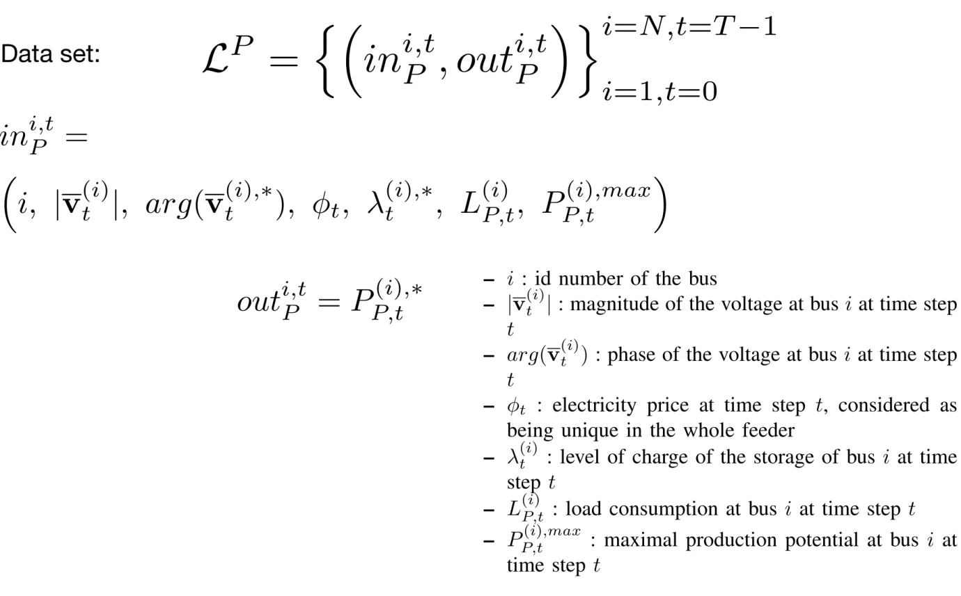
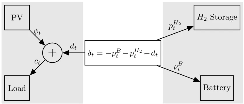
Modeling
N prosumers dynamically interacting with each other over a time horizon T:
where δD_P(i)P,t is the difference between the power injected into the distribution
network and the sum of active power exchanges between the members of the community.
Foreseeing New Control Challenges
in Electricity Prosumer Communities
Fr´ed´eric Olivier
Department of Electrical Engineering and Computer Science
University of Li`ege, Belgium Email: [email protected]
Damien Ernst
Department of Electrical Engineering and Computer Science
University of Li`ege, Belgium Email: [email protected]
Rapha¨el Fonteneau
Department of Electrical Engineering and Computer Science
University of Li`ege, Belgium Email: [email protected]
Abstract—This paper is dedicated to electricity prosumer communities, which are group of people producing, sharing and consuming electricity locally. This paper focuses on building a rigorous mathematical framework in order to formalise sequen-tial decision marking problems that may soon be encountered within electricity prosumer communities. After introducing our formalism, we propose a set of optimisation problems reflecting several types of theoretically optimal behaviours for energy exchanges between prosumers. We finally provide an illustration of a decision making strategy allowing a prosumer community to generate more distributed electricity (compared to commonly applied strategies) by mitigating over-voltages over a low-voltage feeder.
I. INTRODUCTION
This paper is dedicated to electricity prosumer communi-ties, i.e. groups of people producing, sharing and consuming electricity locally. One of the main trigger of the emergence of the concept of energy communities is distributed electricity generation. By distributed electricity generation, we mainly mean PhotoVoltaic (PV) units, small wind turbines and Com-bined Heat and Power (CHP) that may be installed close to consumers. A cost-drop has been observed in the past recent years, especially in the cost for producing PV panels. In addition to this, promises raised by recent advances made in the field of Electric Vehicles (EVs) and batteries may also emphasise in the coming years the metamorphosis of the elec-tricity production, distribution and consumption landscape that is already happening. In addition to electricity production and storage technology improvements, one should also mention the emergence of information technologies facilitating interactions between prosumers [1]. One should also note the existence of projects related to the use of distributed ledgers for managing energy exchanges [2] between microgrids1.
In this paper, we consider that the energy community is composed of prosumers that are connected to the same low-voltage distribution network and that there is only one point of connection between the community and the power system, which is called the root connection of the com-munity. This means that the power exchanges between the prosumers do not transit through distribution transformers. Our goal is to propose a rigorous mathematical framework
1See for instance the Brooklyn Microgrid project.
for studying energy prosumer communities. We first propose a mathematical framework for modelling the interaction between several prosumers. We then formalise a few optimisation problem targeting several different objectives (eg, maximising the “green” production, taking losses into account, optimising costs and revenues, etc). We propose a first community-based decision making strategy for optimising “green” production within a low-voltage feeder.
II. FORMALIZING AN ENERGY PROSUMER COMMUNITY
A. The Prosumers
We consider a set of N 2 N prosumers dynamically interacting with each other over a time horion T 2 N. We first consider a discrete time setting : t 2 {0, . . . , T 1}. In the following, power related variables are average values over a time window , corresponding to the time interval between two time steps. At every time-step t 2 {0, . . . , T 1}, each prosumer is characterised by active (resp. reactive2) power variables subscripted by P (resp. Q): production variables PP,t(i) and PQ,t(i) , (note that PQ,t(i) is positive when producing reactive power and negative when consuming it), a power injected into a storing device St(i), the level of charge of the storage device (i)t , loads (or consumptions) L(i)P,t and L(i)Q,t, and powers injected into the distribution network DP,t(i) and DQ,t(i) .
We assume that all prosumers may interact with each other. In particular, we denote by ✓t(i!j) the (positive) power that is transferred at time t from prosumer (i) to prosumer (j), (i, j) 2 {1, . . . , N}2. In the same time, prosumer (j) receives a (positive) power from prosumer (i) denoted by ✓t(j i). By definition, we have:
8(i, j) 2 {1, . . . , N}2, 8t 2 {0, . . . , T 1},
✓t(i!j) = ✓t(j i) (1) with the convention that ✓t(i!i) = 0, ✓t(i i) = 0 8i, t.
2Considering reactive power is important as it allows greater flexibility in
the management of the networks and can allow the community to have more leverage on the network constraints.
At every time step, the active power that is produced by prosumer (i) must satisfy the following relationship:
8t, i, PP,t(i) = L(i)P,t + DP,t(i) + SP,t(i) (2) 8t, i, DP,t(i) = N X j=1 ⇣ ✓t(i!j) ✓t(i j)⌘ + DP,t(i) (3) where DP,t(i) is the difference between the power injected into the distribution network and the sum of active power exchanges between the members of the community. Note that, in the case where the local production PP,t(i) is not high enough to cover the load L(i)P,t, the variable DP,t(i) may take some negative values (depending also on the amount of power that can be taken from the storage device).
The conservation of reactive power at the prosumer’s loca-tion induces the following:
8t, i, PQ,t(i) = L(i)Q,t + DQ,t(i) (4) In this paper, we focus on energy exchanges among pro-sumers. For this reason, we choose to neglect electricity losses that are not directly associated with energy exchanges between prosumers.
Prosumers may not always be able to produce electricity at its maximal potential (for instance, PV production may be curtailed when, for instance, the local storage device is fully recharged, no exchanges between prosumers are possible, and an overvoltages are observed on the distribution network be-cause many prosumers are injecting together simultaneously: such a situation may appear on sunny days [3], [4]). Thus, for every prosumer, for every time-step, we define the maximal production potential which depends on hardware and weather data:
8t, i PP,t(i) PP,t(i),max (5) Pt(i),max may be influenced by several parameters, in particular weather conditions.
The reactive power is limited by the capability curve of the distributed energy ressources. It depends on the minimum power factor, the maximum apparent power and the current active power production.
8t, i PQ,t(i) PQ(i),max ⇣PP,t(i)⌘ (6) The injected power into the storage device is capped by a factor that mainly depends on the characteristics of the storage device and its current level of charge:
8t, i, St(i) S(i),max
⇣ (i)
t
⌘
(7) The injected power into the distribution network is also capped, depending on the load and local production, charac-teristics and level of charge of the battery, and also additional (stochastic) variables, such as weather, that may influence the voltage of the low-voltage feeder (e.g. unbability to inject
power into the network if the voltage is higher than 1.1 p.u.), thus potentially preventing from power injection:
8t, i, DP,t(i)
DP(i),max ⇣PP,t(i), PQ,t(i) , L(i)P,t, L(i)Q,t, St(i), DP,t(j6=i), DQ,t(j6=i)⌘ (8) 8t, i, DQ,t(i)
DQ(i),max ⇣PP,t(i), PQ,t(i) , L(i)P,t, L(i)Q,t, St(i), DP,t(j6=i), DQ,t(j6=i)⌘ (9) The level of charge of the storage capacity is also bounded: 8t, i 0 (i)t (i),max (10)
B. The Community
Everything that is not produced by the community has to come from the distribution network through the root of the community. By measuring the active and reactive power transfer at the root, and by comparing the measured powers to those measured at the prosumers’ location, we can deduce the losses and the import of reactive power:
8t ⇤(c)P,t = DP,t(c) N X i=1 DP,t(i) (11) 8t ⇤(c)Q,t = DQ,t(c) N X i=1 DQ,t(i) (12) where ⇤(c)P,t (resp. ⇤(c)Q,t) denotes the overall losses inside the electrical network of the community (resp. reactive power absorbed by the community network lines), DP,t(c) (resp. DP,t(c)) is the active (resp. reactive) power measured at the root of the community.
C. Costs and Revenues
At every time-step, we define a set of price variables, expressed in e/kWh. First, each prosumer (i) may purchase electricity from its retailer at a specific price P rt(D!i). Also, each prosumer (i) may buy electricity from prosumer (j) (j 6= i) at a price P rt(j!i). Each prosumer (i) may also sell
electricity to the (distribution) network at a price P rt(i!D), and to other prosumers at a price P rt(i!j). By convention, we assume that all prices considered in the paper are positive. From time t to t + 1, a prosumer (i) will suffer the following cost:
c(i)t =
✓
max ⇣ Dt(i), 0⌘ P rt(D!i) + PNj=1 max ⇣✓t(i j), 0⌘ P rt(j!i)
◆
(13) In the same time, it will also receive the following revenues:
rt(i) = ✓ max ⇣ Dt(i), 0⌘ P rt(i!D) + PNj=1 max ⇣✓t(j i), 0⌘ P rt(i j) ◆ (14)
Modeling
Conservation of reactive power at the prosumer’s location
Other power-related constraints:
At every time step, the active power that is produced by
prosumer (i) must satisfy the following relationship:
8t, i, P
P,t(i)= L
(i)P,t+ D
P,t(i)+ S
P,t(i)(2)
8t, i, D
P,t(i)=
NX
j=1⇣
✓
t(i!j)✓
t(i j)⌘
+ D
P,t(i)(3)
where D
P,t(i)is the difference between the power injected
into the distribution network and the sum of active power
exchanges between the members of the community. Note that,
in the case where the local production P
P,t(i)is not high enough
to cover the load L
(i)P,t, the variable D
P,t(i)may take some
negative values (depending also on the amount of power that
can be taken from the storage device).
The conservation of reactive power at the prosumer’s
loca-tion induces the following:
8t, i, P
Q,t(i)= L
(i)Q,t+ D
Q,t(i)(4)
In this paper, we focus on energy exchanges among
pro-sumers. For this reason, we choose to neglect electricity losses
that are not directly associated with energy exchanges between
prosumers.
Prosumers may not always be able to produce electricity
at its maximal potential (for instance, PV production may be
curtailed when, for instance, the local storage device is fully
recharged, no exchanges between prosumers are possible, and
an overvoltages are observed on the distribution network
be-cause many prosumers are injecting together simultaneously:
such a situation may appear on sunny days [3], [4]). Thus, for
every prosumer, for every time-step, we define the maximal
production potential which depends on hardware and weather
data:
8t, i P
P,t(i) P
P,t(i),max(5)
P
t(i),maxmay be influenced by several parameters, in particular
weather conditions.
The reactive power is limited by the capability curve of
the distributed energy ressources. It depends on the minimum
power factor, the maximum apparent power and the current
active power production.
8t, i P
Q,t(i) P
Q(i),max⇣
P
P,t(i)⌘
(6)
The injected power into the storage device is capped by a
factor that mainly depends on the characteristics of the storage
device and its current level of charge:
8t, i, S
t(i) S
(i),max⇣
(i)t
⌘
(7)
The injected power into the distribution network is also
capped, depending on the load and local production,
charac-teristics and level of charge of the battery, and also additional
(stochastic) variables, such as weather, that may influence the
voltage of the low-voltage feeder (e.g. unbability to inject
power into the network if the voltage is higher than 1.1 p.u.),
thus potentially preventing from power injection:
8t, i,
D
P,t(i) D
P(i),max⇣
P
P,t(i), P
Q,t(i), L
(i)P,t, L
(i)Q,t, S
t(i), D
P,t(j6=i), D
Q,t(j6=i)⌘
(8)
8t, i,
D
Q,t(i) D
Q(i),max⇣
P
P,t(i), P
Q,t(i), L
(i)P,t, L
(i)Q,t, S
t(i), D
P,t(j6=i), D
Q,t(j6=i)⌘
(9)
The level of charge of the storage capacity is also bounded:
8t, i 0
(i)t
(i),max(10)
B. The Community
Everything that is not produced by the community has
to come from the distribution network through the root of
the community. By measuring the active and reactive power
transfer at the root, and by comparing the measured powers
to those measured at the prosumers’ location, we can deduce
the losses and the import of reactive power:
8t ⇤
(c)P,t= D
P,t(c) NX
i=1D
P,t(i)(11)
8t ⇤
(c)Q,t= D
(c) Q,t NX
i=1D
Q,t(i)(12)
where ⇤
(c)P,t(resp. ⇤
(c)Q,t) denotes the overall losses inside the
electrical network of the community (resp. reactive power
absorbed by the community network lines), D
P,t(c)(resp. D
P,t(c))
is the active (resp. reactive) power measured at the root of the
community.
C. Costs and Revenues
At every time-step, we define a set of price variables,
expressed in e/kWh. First, each prosumer (i) may purchase
electricity from its retailer at a specific price P r
t(D!i). Also,
each prosumer (i) may buy electricity from prosumer (j)
(j 6= i) at a price P r
t(j!i). Each prosumer (i) may also sell
electricity to the (distribution) network at a price P r
t(i!D),
and to other prosumers at a price P r
t(i!j). By convention,
we assume that all prices considered in the paper are positive.
From time t to t + 1, a prosumer (i) will suffer the following
cost:
c
(i)t=
✓
max
⇣
D
t(i), 0
⌘
P r
t(D!i)+
P
Nj=1max
⇣
✓
t(i j), 0
⌘
P r
t(j!i)◆
(13)
In the same time, it will also receive the following revenues:
r
t(i)=
✓
max
⇣
D
t(i), 0
⌘
P r
t(i!D)+
P
Nj=1max
⇣
✓
t(j i), 0
⌘
P r
t(i j)◆
(14)
At every time step, the active power that is produced by
prosumer (i) must satisfy the following relationship:
8t, i, P
P,t(i)= L
(i) P,t+ D
(i) P,t+ S
(i) P,t(2)
8t, i, D
P,t(i)=
NX
j=1⇣
✓
t(i!j)✓
t(i j)⌘
+ D
P,t(i)(3)
where D
P,t(i)is the difference between the power injected
into the distribution network and the sum of active power
exchanges between the members of the community. Note that,
in the case where the local production P
P,t(i)is not high enough
to cover the load L
(i)P,t, the variable D
P,t(i)may take some
negative values (depending also on the amount of power that
can be taken from the storage device).
The conservation of reactive power at the prosumer’s
loca-tion induces the following:
8t, i, P
Q,t(i)= L
(i)Q,t
+ D
(i)Q,t
(4)
In this paper, we focus on energy exchanges among
pro-sumers. For this reason, we choose to neglect electricity losses
that are not directly associated with energy exchanges between
prosumers.
Prosumers may not always be able to produce electricity
at its maximal potential (for instance, PV production may be
curtailed when, for instance, the local storage device is fully
recharged, no exchanges between prosumers are possible, and
an overvoltages are observed on the distribution network
be-cause many prosumers are injecting together simultaneously:
such a situation may appear on sunny days [3], [4]). Thus, for
every prosumer, for every time-step, we define the maximal
production potential which depends on hardware and weather
data:
8t, i P
P,t(i) P
P,t(i),max(5)
P
t(i),maxmay be influenced by several parameters, in particular
weather conditions.
The reactive power is limited by the capability curve of
the distributed energy ressources. It depends on the minimum
power factor, the maximum apparent power and the current
active power production.
8t, i P
Q,t(i) P
(i),max Q
⇣
P
P,t(i)⌘
(6)
The injected power into the storage device is capped by a
factor that mainly depends on the characteristics of the storage
device and its current level of charge:
8t, i, S
t(i) S
(i),max⇣
(i)t
⌘
(7)
The injected power into the distribution network is also
capped, depending on the load and local production,
charac-teristics and level of charge of the battery, and also additional
(stochastic) variables, such as weather, that may influence the
voltage of the low-voltage feeder (e.g. unbability to inject
power into the network if the voltage is higher than 1.1 p.u.),
thus potentially preventing from power injection:
8t, i,
D
P,t(i) D
P(i),max⇣
P
P,t(i), P
Q,t(i), L
(i)P,t, L
(i)Q,t, S
t(i), D
P,t(j6=i), D
Q,t(j6=i)⌘
(8)
8t, i,
D
Q,t(i) D
Q(i),max⇣
P
P,t(i), P
Q,t(i), L
(i)P,t, L
(i)Q,t, S
t(i), D
P,t(j6=i), D
Q,t(j6=i)⌘
(9)
The level of charge of the storage capacity is also bounded:
8t, i 0
(i)t
(i),max(10)
B. The Community
Everything that is not produced by the community has
to come from the distribution network through the root of
the community. By measuring the active and reactive power
transfer at the root, and by comparing the measured powers
to those measured at the prosumers’ location, we can deduce
the losses and the import of reactive power:
8t ⇤
(c)P,t= D
(c) P,t NX
i=1D
P,t(i)(11)
8t ⇤
(c)Q,t= D
Q,t(c) NX
i=1D
Q,t(i)(12)
where ⇤
(c)P,t(resp. ⇤
(c)Q,t) denotes the overall losses inside the
electrical network of the community (resp. reactive power
absorbed by the community network lines), D
P,t(c)(resp. D
P,t(c))
is the active (resp. reactive) power measured at the root of the
community.
C. Costs and Revenues
At every time-step, we define a set of price variables,
expressed in e/kWh. First, each prosumer (i) may purchase
electricity from its retailer at a specific price P r
t(D!i). Also,
each prosumer (i) may buy electricity from prosumer (j)
(j 6= i) at a price P r
t(j!i). Each prosumer (i) may also sell
electricity to the (distribution) network at a price P r
t(i!D),
and to other prosumers at a price P r
t(i!j). By convention,
we assume that all prices considered in the paper are positive.
From time t to t + 1, a prosumer (i) will suffer the following
cost:
c
(i)t=
✓
max
⇣
D
t(i), 0
⌘
P r
t(D!i)+
P
Nj=1max
⇣
✓
t(i j), 0
⌘
P r
t(j!i)◆
(13)
In the same time, it will also receive the following revenues:
r
t(i)=
✓
max
⇣
D
t(i), 0
⌘
P r
t(i!D)+
P
Nj=1max
⇣
✓
t(j i), 0
⌘
P r
t(i j)◆
(14)
At every time step, the active power that is produced by
prosumer (i) must satisfy the following relationship:
8t, i, P
P,t(i)= L
(i)P,t+ D
P,t(i)+ S
P,t(i)(2)
8t, i, D
P,t(i)=
NX
j=1⇣
✓
t(i!j)✓
t(i j)⌘
+ D
P,t(i)(3)
where D
P,t(i)is the difference between the power injected
into the distribution network and the sum of active power
exchanges between the members of the community. Note that,
in the case where the local production P
P,t(i)is not high enough
to cover the load L
(i)P,t, the variable D
P,t(i)may take some
negative values (depending also on the amount of power that
can be taken from the storage device).
The conservation of reactive power at the prosumer’s
loca-tion induces the following:
8t, i, P
Q,t(i)= L
(i)Q,t+ D
Q,t(i)(4)
In this paper, we focus on energy exchanges among
pro-sumers. For this reason, we choose to neglect electricity losses
that are not directly associated with energy exchanges between
prosumers.
Prosumers may not always be able to produce electricity
at its maximal potential (for instance, PV production may be
curtailed when, for instance, the local storage device is fully
recharged, no exchanges between prosumers are possible, and
an overvoltages are observed on the distribution network
be-cause many prosumers are injecting together simultaneously:
such a situation may appear on sunny days [3], [4]). Thus, for
every prosumer, for every time-step, we define the maximal
production potential which depends on hardware and weather
data:
8t, i P
P,t(i) P
(i),max
P,t
(5)
P
t(i),maxmay be influenced by several parameters, in particular
weather conditions.
The reactive power is limited by the capability curve of
the distributed energy ressources. It depends on the minimum
power factor, the maximum apparent power and the current
active power production.
8t, i P
Q,t(i) P
Q(i),max⇣
P
P,t(i)⌘
(6)
The injected power into the storage device is capped by a
factor that mainly depends on the characteristics of the storage
device and its current level of charge:
8t, i, S
t(i) S
(i),max⇣
(i) t⌘
(7)
The injected power into the distribution network is also
capped, depending on the load and local production,
charac-teristics and level of charge of the battery, and also additional
(stochastic) variables, such as weather, that may influence the
voltage of the low-voltage feeder (e.g. unbability to inject
power into the network if the voltage is higher than 1.1 p.u.),
thus potentially preventing from power injection:
8t, i,
D
P,t(i) D
P(i),max⇣
P
P,t(i), P
Q,t(i), L
(i)P,t, L
(i)Q,t, S
t(i), D
P,t(j6=i), D
Q,t(j6=i)⌘
(8)
8t, i,
D
Q,t(i) D
Q(i),max⇣
P
P,t(i), P
Q,t(i), L
(i)P,t, L
(i)Q,t, S
t(i), D
P,t(j6=i), D
Q,t(j6=i)⌘
(9)
The level of charge of the storage capacity is also bounded:
8t, i 0
(i)t
(i),max(10)
B. The Community
Everything that is not produced by the community has
to come from the distribution network through the root of
the community. By measuring the active and reactive power
transfer at the root, and by comparing the measured powers
to those measured at the prosumers’ location, we can deduce
the losses and the import of reactive power:
8t ⇤
(c)P,t= D
P,t(c) NX
i=1D
P,t(i)(11)
8t ⇤
(c)Q,t= D
Q,t(c) NX
i=1D
Q,t(i)(12)
where ⇤
(c)P,t(resp. ⇤
(c)Q,t) denotes the overall losses inside the
electrical network of the community (resp. reactive power
absorbed by the community network lines), D
P,t(c)(resp. D
P,t(c))
is the active (resp. reactive) power measured at the root of the
community.
C. Costs and Revenues
At every time-step, we define a set of price variables,
expressed in e/kWh. First, each prosumer (i) may purchase
electricity from its retailer at a specific price P r
t(D!i). Also,
each prosumer (i) may buy electricity from prosumer (j)
(j 6= i) at a price P r
t(j!i). Each prosumer (i) may also sell
electricity to the (distribution) network at a price P r
t(i!D),
and to other prosumers at a price P r
t(i!j). By convention,
we assume that all prices considered in the paper are positive.
From time t to t + 1, a prosumer (i) will suffer the following
cost:
c
(i)t=
✓
max
⇣
D
t(i), 0
⌘
P r
t(D!i)+
P
Nj=1max
⇣
✓
t(i j), 0
⌘
P r
t(j!i)◆
(13)
In the same time, it will also receive the following revenues:
r
t(i)=
✓
max
⇣
D
t(i), 0
⌘
P r
t(i!D)+
P
Nj=1max
⇣
✓
t(j i), 0
⌘
P r
t(i j)◆
(14)
At every time step, the active power that is produced by
prosumer (i) must satisfy the following relationship:
8t, i, P
P,t(i)= L
(i)P,t+ D
P,t(i)+ S
P,t(i)(2)
8t, i, D
P,t(i)=
NX
j=1⇣
✓
t(i!j)✓
t(i j)⌘
+ D
P,t(i)(3)
where D
P,t(i)is the difference between the power injected
into the distribution network and the sum of active power
exchanges between the members of the community. Note that,
in the case where the local production P
P,t(i)is not high enough
to cover the load L
(i)P,t, the variable D
P,t(i)may take some
negative values (depending also on the amount of power that
can be taken from the storage device).
The conservation of reactive power at the prosumer’s
loca-tion induces the following:
8t, i, P
Q,t(i)= L
(i)Q,t+ D
Q,t(i)(4)
In this paper, we focus on energy exchanges among
pro-sumers. For this reason, we choose to neglect electricity losses
that are not directly associated with energy exchanges between
prosumers.
Prosumers may not always be able to produce electricity
at its maximal potential (for instance, PV production may be
curtailed when, for instance, the local storage device is fully
recharged, no exchanges between prosumers are possible, and
an overvoltages are observed on the distribution network
be-cause many prosumers are injecting together simultaneously:
such a situation may appear on sunny days [3], [4]). Thus, for
every prosumer, for every time-step, we define the maximal
production potential which depends on hardware and weather
data:
8t, i P
P,t(i) P
P,t(i),max(5)
P
t(i),maxmay be influenced by several parameters, in particular
weather conditions.
The reactive power is limited by the capability curve of
the distributed energy ressources. It depends on the minimum
power factor, the maximum apparent power and the current
active power production.
8t, i P
Q,t(i) P
Q(i),max⇣
P
P,t(i)⌘
(6)
The injected power into the storage device is capped by a
factor that mainly depends on the characteristics of the storage
device and its current level of charge:
8t, i, S
t(i) S
(i),max⇣
(i)t
⌘
(7)
The injected power into the distribution network is also
capped, depending on the load and local production,
charac-teristics and level of charge of the battery, and also additional
(stochastic) variables, such as weather, that may influence the
voltage of the low-voltage feeder (e.g. unbability to inject
power into the network if the voltage is higher than 1.1 p.u.),
thus potentially preventing from power injection:
8t, i,
D
P,t(i) D
P(i),max⇣
P
P,t(i), P
Q,t(i), L
(i)P,t, L
(i)Q,t, S
t(i), D
P,t(j6=i), D
Q,t(j6=i)⌘
(8)
8t, i,
D
Q,t(i) D
Q(i),max⇣
P
P,t(i), P
Q,t(i), L
(i)P,t, L
(i)Q,t, S
t(i), D
P,t(j6=i), D
Q,t(j6=i)⌘
(9)
The level of charge of the storage capacity is also bounded:
8t, i 0
(i)t
(i),max(10)
B. The Community
Everything that is not produced by the community has
to come from the distribution network through the root of
the community. By measuring the active and reactive power
transfer at the root, and by comparing the measured powers
to those measured at the prosumers’ location, we can deduce
the losses and the import of reactive power:
8t ⇤
(c)P,t= D
P,t(c) NX
i=1D
P,t(i)(11)
8t ⇤
(c)Q,t= D
Q,t(c) NX
i=1D
Q,t(i)(12)
where ⇤
(c)P,t(resp. ⇤
(c)Q,t) denotes the overall losses inside the
electrical network of the community (resp. reactive power
absorbed by the community network lines), D
P,t(c)(resp. D
P,t(c))
is the active (resp. reactive) power measured at the root of the
community.
C. Costs and Revenues
At every time-step, we define a set of price variables,
expressed in e/kWh. First, each prosumer (i) may purchase
electricity from its retailer at a specific price P r
t(D!i). Also,
each prosumer (i) may buy electricity from prosumer (j)
(j 6= i) at a price P r
t(j!i). Each prosumer (i) may also sell
electricity to the (distribution) network at a price P r
t(i!D),
and to other prosumers at a price P r
t(i!j). By convention,
we assume that all prices considered in the paper are positive.
From time t to t + 1, a prosumer (i) will suffer the following
cost:
c
(i)t=
✓
max
⇣
D
t(i), 0
⌘
P r
t(D!i)+
P
Nj=1max
⇣
✓
t(i j), 0
⌘
P r
t(j!i)◆
(13)
In the same time, it will also receive the following revenues:
r
t(i)=
✓
max
⇣
D
t(i), 0
⌘
P r
t(i!D)+
P
Nj=1max
⇣
✓
t(j i), 0
⌘
P r
t(i j)◆
(14)
Modeling
Network voltage
At every time step, the active power that is produced by
prosumer (i) must satisfy the following relationship:
8t, i, P
P,t(i)= L
(i)P,t+ D
P,t(i)+ S
P,t(i)(2)
8t, i, D
P,t(i)=
NX
j=1⇣
✓
t(i!j)✓
t(i j)⌘
+ D
P,t(i)(3)
where D
P,t(i)is the difference between the power injected
into the distribution network and the sum of active power
exchanges between the members of the community. Note that,
in the case where the local production P
P,t(i)is not high enough
to cover the load L
(i)P,t, the variable D
P,t(i)may take some
negative values (depending also on the amount of power that
can be taken from the storage device).
The conservation of reactive power at the prosumer’s
loca-tion induces the following:
8t, i, P
Q,t(i)= L
(i)Q,t+ D
Q,t(i)(4)
In this paper, we focus on energy exchanges among
pro-sumers. For this reason, we choose to neglect electricity losses
that are not directly associated with energy exchanges between
prosumers.
Prosumers may not always be able to produce electricity
at its maximal potential (for instance, PV production may be
curtailed when, for instance, the local storage device is fully
recharged, no exchanges between prosumers are possible, and
an overvoltages are observed on the distribution network
be-cause many prosumers are injecting together simultaneously:
such a situation may appear on sunny days [3], [4]). Thus, for
every prosumer, for every time-step, we define the maximal
production potential which depends on hardware and weather
data:
8t, i P
P,t(i) P
P,t(i),max(5)
P
t(i),maxmay be influenced by several parameters, in particular
weather conditions.
The reactive power is limited by the capability curve of
the distributed energy ressources. It depends on the minimum
power factor, the maximum apparent power and the current
active power production.
8t, i P
Q,t(i) P
Q(i),max⇣
P
P,t(i)⌘
(6)
The injected power into the storage device is capped by a
factor that mainly depends on the characteristics of the storage
device and its current level of charge:
8t, i, S
t(i) S
(i),max⇣
(i)t
⌘
(7)
The injected power into the distribution network is also
capped, depending on the load and local production,
charac-teristics and level of charge of the battery, and also additional
(stochastic) variables, such as weather, that may influence the
voltage of the low-voltage feeder (e.g. unbability to inject
power into the network if the voltage is higher than 1.1 p.u.),
thus potentially preventing from power injection:
8t, i,
D
P,t(i) D
P(i),max⇣
P
P,t(i), P
Q,t(i), L
(i)P,t, L
(i)Q,t, S
t(i), D
P,t(j6=i), D
Q,t(j6=i)⌘
(8)
8t, i,
D
Q,t(i) D
Q(i),max⇣
P
P,t(i), P
Q,t(i), L
(i)P,t, L
(i)Q,t, S
t(i), D
P,t(j6=i), D
Q,t(j6=i)⌘
(9)
The level of charge of the storage capacity is also bounded:
8t, i 0
(i)t
(i),max(10)
B. The Community
Everything that is not produced by the community has
to come from the distribution network through the root of
the community. By measuring the active and reactive power
transfer at the root, and by comparing the measured powers
to those measured at the prosumers’ location, we can deduce
the losses and the import of reactive power:
8t ⇤
(c)P,t= D
P,t(c) NX
i=1D
P,t(i)(11)
8t ⇤
(c)Q,t= D
Q,t(c) NX
i=1D
Q,t(i)(12)
where ⇤
(c)P,t(resp. ⇤
(c)Q,t) denotes the overall losses inside the
electrical network of the community (resp. reactive power
absorbed by the community network lines), D
P,t(c)(resp. D
P,t(c))
is the active (resp. reactive) power measured at the root of the
community.
C. Costs and Revenues
At every time-step, we define a set of price variables,
expressed in e/kWh. First, each prosumer (i) may purchase
electricity from its retailer at a specific price P r
t(D!i). Also,
each prosumer (i) may buy electricity from prosumer (j)
(j 6= i) at a price P r
t(j!i). Each prosumer (i) may also sell
electricity to the (distribution) network at a price P r
t(i!D),
and to other prosumers at a price P r
t(i!j). By convention,
we assume that all prices considered in the paper are positive.
From time t to t + 1, a prosumer (i) will suffer the following
cost:
c
(i)t=
✓
max
⇣
D
t(i), 0
⌘
P r
t(D!i)+
P
Nj=1max
⇣
✓
t(i j), 0
⌘
P r
t(j!i)◆
(13)
In the same time, it will also receive the following revenues:
r
t(i)=
✓
max
⇣
D
t(i), 0
⌘
P r
t(i!D)+
P
Nj=1max
⇣
✓
t(j i), 0
⌘
P r
t(i j)◆
(14)
Modeling
Losses « at the root of the community » :
where D(c)P,t (resp. D(c)Q,t) is the active (resp. reactive) power measured at the
root of the community.
At every time step, the active power that is produced by
prosumer (i) must satisfy the following relationship:
8t, i, P
P,t(i)= L
(i)P,t+ D
P,t(i)+ S
P,t(i)(2)
8t, i, D
P,t(i)=
NX
j=1⇣
✓
t(i!j)✓
t(i j)⌘
+ D
P,t(i)(3)
where D
P,t(i)is the difference between the power injected
into the distribution network and the sum of active power
exchanges between the members of the community. Note that,
in the case where the local production P
P,t(i)is not high enough
to cover the load L
(i)P,t, the variable D
P,t(i)may take some
negative values (depending also on the amount of power that
can be taken from the storage device).
The conservation of reactive power at the prosumer’s
loca-tion induces the following:
8t, i, P
Q,t(i)= L
(i)Q,t+ D
Q,t(i)(4)
In this paper, we focus on energy exchanges among
pro-sumers. For this reason, we choose to neglect electricity losses
that are not directly associated with energy exchanges between
prosumers.
Prosumers may not always be able to produce electricity
at its maximal potential (for instance, PV production may be
curtailed when, for instance, the local storage device is fully
recharged, no exchanges between prosumers are possible, and
an overvoltages are observed on the distribution network
be-cause many prosumers are injecting together simultaneously:
such a situation may appear on sunny days [3], [4]). Thus, for
every prosumer, for every time-step, we define the maximal
production potential which depends on hardware and weather
data:
8t, i P
P,t(i) P
(i),max
P,t
(5)
P
t(i),maxmay be influenced by several parameters, in particular
weather conditions.
The reactive power is limited by the capability curve of
the distributed energy ressources. It depends on the minimum
power factor, the maximum apparent power and the current
active power production.
8t, i P
Q,t(i) P
(i),max Q
⇣
P
P,t(i)⌘
(6)
The injected power into the storage device is capped by a
factor that mainly depends on the characteristics of the storage
device and its current level of charge:
8t, i, S
t(i) S
(i),max⇣
(i)t