CALCULATION OF THE SCATTERING COEFFICIENT
OF A SINE-SHAPED SURFACE
BY SOLVING THE HELMHOLTZ INTEGRAL
JJ Embrechts University of Liege, Dept of Electrical Engineering and Computer Science, Belgium L. De Geetere K.U.Leuven, Laboratory of Building Physics and Laboratory of Acoustics, Belgium G. Vermeir K.U.Leuven, Laboratory of Building Physics and Laboratory of Acoustics, Belgium
1 INTRODUCTION
Measurements of the random-incidence scattering coefficients of a sine-shaped surface (3 meter diameter) have been performed in real-size reverberant rooms, according to the procedure described in the ISO document ISO/DIS 17497-11. A round-robin test has been organized, using two sets of measuring instruments, two similar sine-shaped samples and two reverberation rooms belonging to the acoustics laboratories of the universities of Liege and Leuven.
The motivation was to investigate the feasibility of such a real-scale experiment and the practical problems which could arise during its application. These measurements and their results have already been presented at Forum Acusticum in Sevilla2,3.
It was also intended to obtain theoretical values to which the measured scattering coefficients could be compared and which would help us to analyze the degree of accuracy of our measurements.
Unfortunately, there’s no simple (analytical) solution for the theoretical problem of the scattering of a plane sound wave (or random-incidence sound field) by a perfectly hard sine-shaped surface. Therefore, two numerical methods have been applied : BEM (boundary element method) and the Helmholtz integral method.
This paper reports on the Helmholtz integral method, while another paper describes the results obtained by BEM4.
2
THE HELMHOLTZ INTEGRAL
In a 3D scattering problem, the pressure ps(R) scattered by a finite rough surface at point R (see fig.
1) is given by the Helmholtz integral formula5,eq.(19.7) :
jkD S s s s
e
D
G
dS
n
dS
p
G
n
G
dS
p
R
p
(
)
(
)
1
4
1
)
(
⎟
=
⎠
⎞
⎜
⎝
⎛
∂
∂
−
∂
∂
=
∫
π
(1)in which ps(dS) is the scattered sound pressure at the surface element dS, G is the 3D Green
function and (δ/δn) represents the derivative along the outward normal to the rough surface at dS. Also, D is the distance between point R and the surface element dS.
Figure 1 : Scattering geometry for a plane wave incident along vector
k
1. The receiver R lies along the scattering directionk
2.To solve integral (1), the main difficulty is of course to derive the pressure and its gradient on the surface. For example, it can be assumed that these are given by their so-called “tangent-plane” approximation6. This assumption holds for “smoothly undulating” surfaces and leads to the Kirchhoff Approximation (KA) method (in fact, eq.(1) already includes another Kirchhoff assumption, i.e. that the pressure field is unperturbed in the plane z=0 outside S0, an assumption which is not necessary
for infinite surfaces).
When the “tangent-plane” approximation is applied in (1), then the scattered pressure is expressed by6 :
( )
∫
=
0.
)
(
. S r v j sR
K
e
v
dxdy
p
γ
(2)In this equation, the sound pressure is evaluated in the Fraunhofer zone, i.e. at great distance from all points of the finite rough surface. The coefficient K is a constant depending on the complex amplitude of the incident plane wave and on the distance R0 between the center of the surface and
the receiver6. The vector
v
is the difference between the incidence vectork
1 and the scattering vectork
2 (both vectors have a magnitude of k=2π/λ). The z-coordinate of the position vectorr
is given by the profile of the rough surface z=ξ(x,y). Finally,γ
is a vector perpendicular to the rough surface at dS, with coordinates (-dξ/dx,-dξ/dy,1). It is important to notice that (2) has been expressed here for perfectly hard finite rough surfaces.Further developments of this paper will be mainly dedicated to the solutions of the KA method (2). But, as will be seen later, the conditions of validity of this approximation are not fully satisfied by the roughness profile of our test sample, and it is therefore interesting to consider other methods.
One of them which seems particularly attractive has been developed by Holford7, based on works by Urusovskii published in the late sixties. This method is also a solution of the Helmholtz integral, but taking into account the periodicity of the sine-shaped profile. The pressure field on the surface is here expressed as an infinite sum of exponential terms, whose complex amplitudes are determined by a (theoretically infinite) system of algebraic equations. Numerical techniques can be used to approach the exact solution.
Most developments in the original Holford’s paper have been dedicated to pressure-release surfaces. To obtain results for a perfectly hard surface, we have applied the method suggested in Holford’s appendix A, which holds for any impedance boundary condition. However, Holford’s method is only valid for infinite surfaces, while our test sample has a finite diameter of 3 meter. A careful interpretation of the results will therefore be necessary during the comparison with the measured values of the scattering coefficient.
3
RESULTS OF THE K.A. METHOD
3.1 The “characteristic function” model
The numerical solution of (2) gives the scattered pressure for any direction of incidence (
k
1)
and scattering (k
2). Inputting this pressure distribution in the Mommertz formula6 gives the scattering coefficient δ, as a function of incidence (k
1) and, of course, frequency. Finally, therandom-incidence scattering coefficient is obtained by numerical integration over all vectors
k
1, using theParis formula, as for the random-incidence absorption coefficient.
Instead of numerically solving eq. (2), a more efficient and intuitive method has been used here. The “characteristic function” model has been developed by Embrechts et al6, for finite surfaces whose dimensions are “much greater” than the wavelength. According to this model, the scattering coefficient is directly given by :
2 ) ( cos 2 0 1 0 1
1
1
)
,
(
=
−
∫
− S x jkdxdy
e
S
k
θξθ
δ
(3)The roughness profile of our test sample is one-dimensional and expressed by ξ(x)=Hcos(2πx/Λ), with H=0.0255m and Λ=0.177m.
The validity of (3) has been investigated by computing the scattering coefficient for some directions of incidence, using the complete Kirchhoff procedure as described above. An excellent correspondence was observed between both techniques, in the frequency interval [315 Hz-8000 Hz].
The “characteristic function” model states that the scattering coefficient depends on the angle of incidence θ1 (see fig.1), but not on the azimuthal orientation of the incident wave. This conclusion
could be hard to believe and is, in fact, not particular to this model, but well to the more general KA method. It is only an approximation that remains valid as long as KA conditions of validity are satisfied.
This in turn greatly simplifies the random-incidence computations through Paris formula. The results obtained for our sine-shaped surface are shown in figure 2, for several angles of incidence (from 5 to 85 degrees). In this figure are also shown the random-incidence scattering coefficients obtained by integrating over θ1.
These results will be compared with similar values obtained by measurements and other numerical techniques. Table 1 summarizes the conditions in which the scattering coefficients have been derived. Indeed, each method has its own assumptions and these must be clearly understood before comparing the results. For example, unlike the “characteristic function” model, BEM needs to compute the 3D scattering distribution (on a given receiver mesh) before integrating over all directions of scattering to obtain the scattering coefficient.
Sine-shaped surface scattering coefficients - Kirchhoff Approxim ation 0 10 20 30 40 50 60 70 80 90 100 125 157 198 250 315 397 500 630 794 1000 1260 1587 2000 2520 3175 4000 5040 6350 8000 10079 12699 16000 freq (Hz) percents 5 deg 15 25 35 45 55 65 75 85 random incidence
Figure 2
:
Scattering coefficients (in percents) of the sine-shaped sample predicted by the Kirchhoff Approximation (“characteristic function” model), for several conditions of sound wave incidence.Table 1 : Conditions in which the scattering coefficients have been obtained by each method
Method Surface size Incident field Receiver mesh KA (“characteristic
function”)
Finite Plane-wave and 3D random (*)
Not necessary : see eq. (3) BEM Finite Plane-wave and
3D random (**)
Every 2 degrees in elevation and azimuth Holford Infinite Plane-wave and
3D random (***)
Not necessary : see section 4 Measurements in the
reverberation room
Finite 3D random Only one receiver position1
(*) The random-incidence scattering coefficient is here obtained by analytical integration over elevation and azimuth incidence angles.
(**) The random incident field is here modeled by a source mesh (a source every 10 degrees in elevation and azimuth angles), followed by numerical integration.
(***) Not available yet, but Holford’s method allows 3D incidence integration.
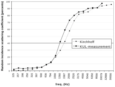
Figure 3 compares the KA results with the random-incidence scattering coefficients measured in the real-scale reverberation rooms (average values obtained by the K.U. Leuven measurement technique). At first glance, the correspondence between both set of coefficients is fairly good, except in the interval [1260Hz-4000Hz], where the KA method predicts slightly lower values than the measurements.
However, further comparisons with BEM results4 (obtained in the “transition” region 500-2000 Hz) indicated that indeed, KA gives underestimated random-incidence scattering coefficients in this
transition region, but also that the individual plane wave incidence curves (fig. 2) presented quite large deviations with BEM predictions. These results lead us to investigate further and analyze the validity of KA application for our sine-shaped surface.
0 10 20 30 40 50 60 70 80 90 100 1 25 1 57 1 9 8 2 5 0 31 5 3 97 5 00 6 3 0 7 9 4 1 00 0 1 2 60 1 5 8 7 20 0 0 2 52 0 3 17 5 4 0 00 5 0 4 0 63 5 0 8 00 0 1 0 07 9 1 2 6 99 16 0 0 0 freq. (H z)
Random incidence scattering
coefficient (percents)
K irchhoff
K U L-m easurem ent
Figure 3
:
Comparison of the random-incidence scattering coefficients computed by the Kirchhoff Approximation and those measured in the real-scale reverberation rooms by the K.U. Leuven measurement technique.3.2 The validity of the Kirchhoff approximation
The conditions of validity of (2) are not well established, even today. For gaussian surfaces, Thorsos8 concluded that KA gives accurate results if :
- the r.m.s. slope of the surface does not exceed 0.35;
-
the correlation length (which, for gaussian surfaces, is2
times the ratio of r.m.s. height to r.m.s. slope) is greater than the wavelength;-
the angles of incidence and scattering are less than 60 degrees.Applying similar conditions to our sine-shaped sample leads to :
- the r.m.s. slope is
0
.
640
177
.
0
)
0255
.
0
(
2
2=
=
⎟
⎠
⎞
⎜
⎝
⎛
∂
∂
ξ
π
x
;-
the quantity equivalent to the correlation length should be :0
.
04
m
640
.
0
0255
.
0
=
(fmin=8.5 kHz).This simple evaluation seems to indicate that the limits of K.A. have been reached in this case. Therefore, the theoretical values presented in figure 2 must be considered with precaution, even if they give a fairly good agreement (in average) with the measured values.
Unfortunately, BEM techniques cannot easily be applied above 2 kHz. Then, they are not able to confirm KA results at high frequencies. Other methods should be applied for that purpose.
4 HOLFORD’S
METHOD
The method developed by Holford7 has been applied here, since our test sample has a periodic roughness profile. As indicated above however, this method only holds for infinite surfaces, whereas our circular sample has a well finite (3 meter) diameter. It is recalled here that the ISO measurement procedure has been defined to give measurement results which are representative for an infinitely large surface, and this already suggests that the measured scattering coefficients should approach the values derived by the Holford’s method in order to fulfill this requirement.
At the time of writing this paper, the complete results are not yet available. But some interesting considerations can already be expressed.
First, this method predicts that the scattered field consists of discrete plane waves : one in the specular direction, other propagating waves in directions given by the grating equation
...
,
2
,
1
sin
sin
1=
±
±
Λ
+
=
n
n
nλ
θ
θ
(4)and, finally, surfaces waves which do not radiate energy away from the surface. Therefore, the scattering coefficient is here simply 1 minus the ratio of the energy radiated by the specular plane wave to the total reflected energy.
If λ/Λ>2 in (4), there’s no propagating wave other than the specular wave, and then the scattering coefficient must be zero. This occurs in our case for frequencies less than 960 Hz : for f<960 Hz,
there should be no scattering by an infinite sine-shaped surface having the roughness profile
described above (with H=0.0255m and Λ=0.177m). This is in contradiction with KA results in fig. 2, where it can be seen that the scattering coefficient is rather weak, but not zero. But, this is also in contradiction with the measurements (see fig. 3) and with BEM results (see fig.4).
It therefore appears that the weak scattering observed before 960 Hz should be related in some way to the finite size of the surface, rather than to its roughness profile. Another explanation could be that the “uncorrelated reflected energy” computed or measured by the ISO method should not be fully attributed to the influence of the roughness profile : there comes again the question of how to extract the “diffuse” component from a global reflected pressure distribution ? If this seems to be obvious for an infinite periodic surface, on the other hand there’s no clear separation of the specular and diffuse pressures for a finite surface.
Second observation : the first results obtained by Holford’s method application show quite significant deviations with those obtained by the KA method for the finite size surface (compare fig. 4 and fig. 2). In particular, Holford’s method predicts very weak scattering (i.e. a strong specular reflection) in a narrow frequency band, around some discrete frequencies at which a new scattered plane wave is generated in the direction θn=-90 degrees (in fig. 4, n=-2).
On the other hand, the BEM simulations seem to give results which are in fairly good agreement with those of Holford, at least in the conditions of the fig.4 experiment. The measured incidence coefficients cannot be compared at this moment, since all the values needed for random-incidence integration are not yet available.
Incidence 60 deg. from perpendicular, Az0 deg 0 0.1 0.2 0.3 0.4 0.5 0.6 0.7 0.8 0.9 1 1.1 0 500 1000 1500 2000 2500 3000 Hz Sc a tte ring c o e ffic ie n t Holford's method 3D BEM
Figure 4 : Scattering coefficients of the sine-shaped surface computed by Holford’s method (infinite
surface) and 3D BEM (circular sample, 3m diameter). The plane wave is incident along the direction 60 degrees from perpendicular and azimuth 0 degree, which means that the direction of incidence lies in a plane perpendicular to the sine-shaped corrugations.
Third and last observation : Holford’s method gives, in principle, an exact solution. However, the practical application of this method needs some approximations. For example, the exact pressure distribution on the surface is expressed as an infinite sum of exponential terms, whose complex amplitudes are determined by an infinite system of algebraic equations. Obviously, the practical application should restrict the size of this system of equations, introducing a parameter which influences the computed results.
5 CONCLUSION
It is shown in this paper that the theoretical solution of the simple problem of the sound scattering by a sine-shaped surface is not obvious.
However, this solution would be very useful in order to interpret correctly and analyze the accuracy of the random-incidence scattering coefficients measured by the ISO method.
It seems that no particular method is able to generate the exact solution to this theoretical problem, but rather that the conjunction of several results and their careful interpretation could finally lead us to an acceptable approximation at all frequencies.
6 REFERENCES
1. ISO/DIS 17497-1 : Acoustics – Measurement of the sound scattering properties of surfaces – Part 1 : Measurement of the random-incidence scattering coefficient in a reverberation room (2000).
2. J.J. Embrechts, ‘Practical aspects of the ISO procedure for measuring the scattering coefficient in a real-scale experiment’, Proc. Forum Acusticum Sevilla (2002).
3. L. De Geetere and G. Vermeir, ‘Investigations on real-scale experiments for the measurement of the ISO scattering coefficient in the reverberation room’, Proc. Forum Acusticum Sevilla (2002).
4. L. De Geetere, J.J. Embrechts and G. Vermeir, ‘Calculation of the scattering coefficient of a sine-shaped surface by using the 3D BEM method’, Proc. Research Symposium on Acoustic Characteristics of Surfaces, Salford (2003).
5. F.G. Bass and I.M. Fuks. Wave scattering from statistically rough surfaces, Pergamon, Oxford (1979).
6. J.J. Embrechts, D. Archambeau and G.B. Stan, ‘Determination of the scattering coefficient of random rough diffusing surfaces for room acoustics applications’, Acta acustica – Acustica 87 482-494 (2001).
7. R.L. Holford, ‘Scattering of sound waves at a periodic, pressure-release surface : An exact solution’, J. Acoust. Soc. Am. 70(4) 1116-1128 (Oct. 1981).
8. E.I. Thorsos, ‘The validity of the Kirchhoff approximation for rough surface scattering using a gaussian roughness spectrum’, J. Acoust. Soc. Am. 83(1) 78-92 (1988).