Texture evolution during deep-drawing processes
L. Duchêne , A. Godinas, S. Cescotto, A.M. Habraken
Department of Structures, University of Liège, Chemin des Chevreuils 1, 4000 Liège, Belgium
Abstract
This paper presents a constitutive law based on Taylor's model implemented in our non-linear finite element code LAGAMINE. The yield locus is only locally described and a particular interpolation method has been developed. This local yield locus model uses a discrete representation of the material's texture. The interpolation method is presented and a deep-drawing application is simulated in order to show up the influence of the texture evolution during forming processes.
Keywords: Texture evolution; Yield locus; Finite elements; Deep-drawing
1. Statement of the problem
The objective of this research is to integrate the influence of the material's texture into a finite element code. The constitutive law describing the mechanical behaviour of the studied sample is based on a microscopic approach. The computation takes place on the crystallographic level. A large number of crystals must be used to represent correctly the global behaviour. The micro-macro-transition links the global behaviour to the crystallographic results. The full constraint Taylor's model is used for the computation of the microscopic behaviour of each crystal and for the micro-macro-transition. Unfortunately, this model does not lead to a general law with a mathematical formulation of the yield locus. Only one point of the yield locus corresponding to a particular strain rate direction can be computed.
The "direct Taylor's model" assumes that one macroscopic stress results from the average of the microscopic stresses related to each crystal belonging to a set of representative crystals. The computation of the mechanical behaviour involves a large number of crystals and must be repeated for each integration point of the finite element model, for each iteration of each time step. So, such a micro-macro-approach consumes a large amount of computation time and seems therefore impractical.
However, using different simplified approaches, various constitutive laws based on texture analysis have been implemented in the non-linear finite element code LAGAMINE.
Our first step in the integration of the texture effects has been the use of a sixth order series yield locus defined by a least-squares fitting on a large number of points (typically 70,300) in the deviatoric stress space [4]. Those points were calculated by Taylor's model based on an assumed constant texture of the material. This fitting is performed once, outside the FEM code. It provides 210 coefficients to describe the whole yield locus. This method, i.e. a global description of the yield locus, is actually used in the FEM code.
Unfortunately, taking into account the texture evolution effects with this yield locus would imply the computation of the 210 coefficients of the sixth order series for each integration point, each time a texture updating is necessary. This would require an impressive amount of computation and memory storage (210 coefficients for each integration point), which is only partially useful as generally the stress state remains in a local zone of the yield locus. So, two new approaches, where the whole yield locus is unknown, have been investigated.
In the first case, some points in the interesting part of the yield locus are computed with Taylor's model. This local zone of the yield locus is then represented by a set of hyperplanes which are planes defined in the five-dimensional deviatoric stress space. These planes being fitted on Taylor's points.
As it has been shown in [2], the yield locus discontinuities bred by this very simple interpolation method give rise to convergence problems in the finite element code. That is the reason why a second method has been
developed. For that second approach, no yield locus is defined and a direct stress-strain interpolation between Taylor's points is achieved. In this case, the yield stress continuity conditions are fulfilled but, as there is no yield locus formulation, a particular stress integration scheme has to be used.
Both interpolation methods allow us an important computation time reduction with respect to the "direct Taylor's model" application. Taylor's model is only used to compute some points in order to achieve the interpolation. These points must be computed in two cases:
• When the current part of the yield locus does not content anymore the new stress state and that a new local zone of the yield locus is required.
• When the plastic strain significantly deform the material and induce changes in the crystallographic orientations, i.e. when the texture evolves. Indeed, the corresponding mechanical behaviour of the material would no longer be correctly represented by the old points. A texture updating must therefore take place. The part yield locus approach presented in this paper can be placed between the microscopic approach (accurate but very slow) and the global yield locus approach (fast but inaccurate and especially not adapted for texture updating).
This paper describes the stress-strain interpolation method; interested readers can refer to [2,5] for the sixth order and the hyperplanes method. The influence of the texture updating during a forming process has been
highlighted by a deep-drawing simulation. 2. Stress-strain interpolation
2.1. Local description of a scaled yield locus
The yield locus shape is our present goal. The size of the yield locus is defined by a simple scalar power-type hardening law as already proposed by Winters [5]. The method proposed here is more an interpolation approach than a local representation of a scaled yield locus. A "function" locally describing the plastic surface is not developed. Nevertheless, this interpolation method assumes the existence of a yield locus.
Let s*0 be one unit stress vector, direction of the central point of the local part of the yield locus that requires an approximation. s*(i) are five (N) unit stress vectors surrounding s*0 and determining the interpolation domain. They will be called the "domain limit vectors". In practice, the approach has been developed for a N-dimensional space but is directly applied to the five dimensions case, as the goal is to define a local yield locus zone in the deviatoric stress or strain rate space. Hereafter, the notation choice is adapted to the stress space but all the approach can be translated to the strain rate space. The six or N + 1 vectors (five s*(i) and one s*0) have the following properties:
• They are unit vectors:
• There is a common angle between all s :
• There is a common angle between each s*(i) and s*0 :
• They determine a regular domain. These choices induce that the central direction s*0
can be computed as a scaled average of the five (N) limit vectors s*(i):
The angle θ and the parameter β both determine the size of the interpolation domain. They are linked by the relation:
As the N s*(i) vectors are linearly independent, they constitute a vector basis of the N-dimensional space. However, as they are not orthogonal, it is interesting to introduce N new vectors with following orthogonal property:
These vectors are called "contravariant vectors". Eq. (6) implies that these vectors are not unit ones and one can check that they depend linearly from vectors s*(i) and s*0:
The N -coordinates representing any vector V in the s*(i) vector basis:
are determined, thanks to the N ss(i) vectors:
These N η -coordinates are independent to each other; they determine both length and direction of the vector V. It is important to note that for a unit vector V equal to a domain limit vector s*(i) the -coordinates are
The domain limit vectors represent the domain vertices. The N limit boundaries (or edges) of the interpolation domain correspond to one function such that
In fact, the properties associated to isoparametric finite elements are retrieved but extrapolated to N dimensions. The above choices imply that any point belonging to the interpolation domain is associated to positive -coordinates.
One convenient way to determine the five domain limit vectors s*(i) is to focus on one particular central direction s'*0 chosen in such a way that its N components are identical. To provide associated domain limit vectors s'*(i), one computes a linear relation between the central direction and consecutively each vector of the Cartesian basis e(i) :
Then the rotation linking the real required central point s*0 and the particular one s'*0 is computed by
where I is the second order unit tensor. This rotation applies s'*0 on the real central vector s*0:
It also provides the domain limit vectors:
If s*0 and s'*0 are opposite vectors, Eq. (14) is not valid; the domain limit vectors s*(i) can be computed as the opposite of the s'*(i).
This interpolation domain is called a regular one because the angles between the domain limit vectors are identical (see Eq. (2)) and the domain limit vectors are unit vectors. However, it is possible to define an interpolation domain based on limit vectors which are non-uniformly located and non-unit vectors as long as they are linearly independent and not parallel to each other. With such a non-regular domain, the intrinsic coordinates are still available and require the definition of ss vectors (see Eqs. (6), (8) and (9)).
The above considerations are sufficient to understand the interpolation approach that has finally been
implemented in LAGAMINE code. However, it is interesting to note that further details and properties of such parameterisation of an N-dimensional space were further investigated by Godinas [3] and Duchêne [1]. They studied different interpolation methods on the interpolation domain: linear interpolation in Cartesian coordinates or hyperplane model, linear interpolation in spherical coordinates, approach enriched by bubble mode.
Now, let us consider both five-dimensional stress and strain rate space. A regular domain is built in the strain rate space, defined by its five vertices u*(i) (unit vectors). Thanks to five calls to Taylor's model, the associated stress vectors s(i) are defined. At this level, no hardening is assumed, that is why we speak here of a scaled yield locus. These five stress vectors define a non-regular domain in the stress space. In each space, the concept of contravariant vectors from Eq. (6) is applied
The contravariant vectors ss'(i) and ss(i), respectively, computed by Eqs. (18) and (8) differ only because in Eq. (8) unit stress directions s*(i) are used. Here the length of the stress vectors s(i) is an important characteristic as it defines the yield locus anisotropy. These contravariant vectors ss',(i) and uu(i) give in each space, the
-coordinates associated to any stress s or unit strain rate u*:
So any stress vector s or strain rate direction u* can be represented according to the vector basis of their space and the -coordinates:
Physically, one material state corresponds to one stress point and one strain rate direction. In a yield locus formulation, one point on the locus and its normal define both stress and associated strain rate. Here, we work with two interpolation domains and assume that they are physically linked because Taylor's model computes their domain limit vectors. Due to this close link between the two spaces, it is assumed that the -coordinates computed by Eqs. (19) and (20) are equal when physically the stress s and the strain rate direction u* are associated. This property is exactly fulfilled on the domain limit vectors. The stress s(i) corresponds to the strain rate direction u*(i) and their -coordinates are = 1 and = 0 (i j) in both space. Inside the domain, this property is extended by convenience. It is an assumption. The so-called interpolation approach directly derives from this hypothesis of equality and from Eqs. (22) and (19). They provide the interpolation relation:
For each domain, the C matrix is computed once from the stress domain limit vectors s(i) and the contravariant vectors uu(i) associated to the five strain rate vertices u*(i). Inside one domain, Eq. (23) provides the stress state if the strain rate direction is given. The -coordinates computed by Eq. (19) check the domain validity. If values do not belong to the interval [0, 1], then the interpolation approach of Eq. (23) becomes an extrapolation and a new domain is required.
2.2. Updating of the scaled yield locus description
When the available local description of the scaled yield locus does not cover any more the interesting zone, one has to find another local description enclosing the interesting part of the yield locus. Of course the procedure described by Eqs. (12)-(16) could be repeated using one new strain rate direction u* as central point. However, this would provide a new local description forgetting previous information and the discontinuities observed with the hyperplane approach would again appear. Looking at the -coordinate that does not any more belong to [0, 1], one can identify the boundary not respected by the new explored direction. This boundary is identified by N-1 (=4) domain limit vectors and can belong to two regular domains. The two neighbouring domains defined by their common frontier require only one additional domain limit vector to be completely defined. So only one new vertex must be computed by Taylor's model to identify the neighbour domain that probably contains the new explored strain rate direction. In LAGAMINE implementation of the interpolation method, the neighbour domain is checked before the computation of a completely new local domain begins.
2.3. Stress integration scheme
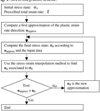
As already mentioned, the stress-strain interpolation relation (Eq. (23)) does not use the concept of yield locus in a classical way. So, a specific integration scheme has been developed. The stress integration scheme
implemented with our interpolation method is completely different from the classical radial return with elastic predictor; the main ideas are summarised in the flowchart of Fig. 1 where obviously, no yield locus formulation is used.
As it has been observed during several finite element simulations, this stress integration scheme is well adapted for a local yield locus description and induces a reasonable number of interpolation domain updating.
At this level, the real stress and not the scaled one is aimed, so the size and the shape of the yield locus cannot anymore be dissociated. As Eq. (23) translates the shape and is assumed to model a reference level of hardening, an additional factor τ is introduced to represent the work hardening:
It plays the role of the hardening and is simply linked to the total polycrystal slip Γ by a Swift law:
Fig. 1. Stress integration scheme.
As in [5], this micro-macro-hardening law is identified by a macroscopic uniaxial tensile test.
2.4. Implementation of the texture updating
In this model, not only is the texture used to predict the plastic behaviour of the material, but also the strain history of each integration point is taken into account in order to update the texture.
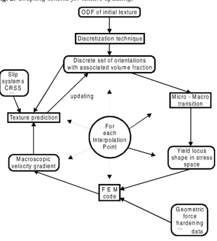
The main ideas of the implementation are summarised in Fig. 2. It should be noticed that the constitutive law in the FEM code is based on the interpolation method described earlier and on Taylor's model applied on the actual set of crystallographic orientations through the yield locus. These crystallographic orientations are represented with the help of the Euler angles ranging from 0° to 360° for and from 0° to 90° for Ø and so as to take crystal cubic symmetry into account but not the sample symmetry. As shown in Fig. 2, the texture updating is achieved outside the main part of the FEM code, for each interpolation point.
During a large finite element simulation, it is not reasonable to achieve a texture updating for each finite element and at the end of each time step. That is the reason why an updating criterion must be used to reduce
computation time. This is still under investigation. At this stage, an updating occurs after a predefined number of time steps. A criterion based on a maximum cumulated plastic strain will also be examined.
The lattice rotation of each crystal, inducing the texture updating, is computed with Taylor's model by subtracting the slip induced spin from the rigid body rotation included in the strain history.
3. Deep-drawing simulations
In order to show up the influence of the texture evolution during a forming process, a deep-drawing simulation has been studied. The material used is a mild steel well adapted for deep-drawing. The numerical data for this steel are obtained from a simple tensile test for the hardening behaviour. As we focus on the texture, the shape of the yield locus is deduced from its orientation distribution function (ODF), which has been measured by X-ray diffraction. The stress-strain interpolation method with and without texture updating is compared to two experimental results and to a classical Hill (1948) constitutive law.
Fig. 2. Coupling scheme for texture updating.
Now, the geometry of the deep-drawing process should be presented. A hemispherical punch with a diameter of 100 mm, a die with a curvature radius of 5 mm and a blankholder are the drawing tools. The drawing ratio is 2.0; the blankholder force is 80 kN; the simulation is achieved up to a drawing depth of 85 mm. This geometry has already been used as the benchmark for the NUMISHEET'99 and ESAFORM'2001 conferences. A Coulomb law is used to model the friction with a coefficient of 0.15.
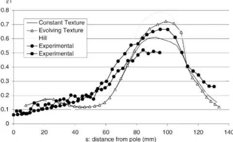
For Hill and texture based laws and for experimental results, the maximum principal strain distribution on a section along the transverse direction is reported in Fig. 3. It should be noticed that the strain is relatively small at the top of the cup (near the pole; for s smaller than 50 mm), while large displacements take place. Indeed, in that part of the cup, the steel sheet is applied against the punch and follows the punch travel without large deformation. Then, at the flange of the cup, the maximum principal strain suddenly increases and is maximum for s equal to 90 mm. This maximum is located at the vertical part of the flange where the cup is free of contact with the punch and the matrix. After the maximum, the principal strain ε1 decreases as the contact with the
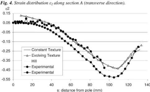
matrix reduces the tension of the sheet. The resulting maximum principal strain obtained with Hill law is a little bit too high while texture based laws are in agreement with experimental results. Fig. 4 shows the second (smallest) principal strain along the same section. Here again, the same evolution can be noticed: low constant value near the pole, followed by a minimum (or a maximum in absolute value) in the flange of the cup and then lower deformations under the blankholder. Looking and together, we can see that four typical regions can be identified:
• Near the pole (s < 40 mm), an equi-biaxial tension state or stretched zone is present
• In the flange (40 < s < 90), increasing tensile and compression strains can be noticed; a restrained zone is determined
• Near the matrix curvature (90 < s < 110), the restrained zone presents a decrease in the absolute value of the strains
• Under the blankholder (110 < s < 135), the compression strain ε2 becomes larger than the tensile
strain and This strain state would give rise to instability and wrinkling without the action of the blankholder.
Fig. 5 shows the third principal strain distribution along section A (transverse direction). It corresponds to the thickness strains. Near the pole, in the equi-biaxial tension strain zone, ε3 is negative: corresponding to a
thickness reduction. Then progressively, ε3 grows and becomes positive (the thickness is increasing during the
process) in the fourth region described here above.
The punch force as a function of the punch travel is presented in Fig. 6. These curves are not linked to the anisotropy of the steel sheet but to the global stiffness of the material and then to the hardening behaviour. It can be noticed that the curve with the evolving texture is very close to the experimental curve; the constant texture is a little bit too low at the end of the process and Hill is too high.
Finally, Figs. 7 and 8 are directly linked to the anisotropy of the steel sheet. For finite element simulations, this anisotropy is introduced in the constitutive law (either the Hill coefficients or the texture data). The flange draw-in is defdraw-ined as the length of the flange that is swallowed under the blankholder. It is the opposite of the earrdraw-ing profile. The experimental results exhibit a maximum draw-in along section B (45°) and lower values along sections A and C. The Hill based constitutive law shows a good draw-in profile (maximum at section B) but the amplitude is too high (variation between the three sections). The draw-in profiles obtained by the texture based laws are very similar to the experimental one. The anisotropy is then well represented by this constitutive law but a shift is observed along both directions: the draw-in is too low with these texture based laws. The behaviour of the material is less ductile numerically than experimentally. The amplitude of the draw-in profile is a little bit higher when the texture is updated during the process.
Fig. 4. Strain distribution ε2 along section A (transverse direction).
Fig. 5. Strain distribution ε3 along section A (transverse direction).
Fig. 7. Flange draw-in at sections A-C.
Fig. 8. Evolution of the Lankford coefficient during deep-drawing.
The draw-in profile can be predicted by the Lankford coefficient. Indeed, a high r value corresponds to a lower thickness deformation during a tensile test. Under the blankholder, the compression strain is predominant
; so, the thickness tends to increase and this effect is more pronounced where the r value is small. Due to the conservation of the volume during plastic deformations, where the thickness is the larger, the draw-in is maximum. Considering a point along section C (rolling direction), the compression strains is acting along a circumferential direction which is the transverse direction. Similarly, for section A, the compression direction is the rolling direction and for section B, it is the direction at 45° from the rolling direction.
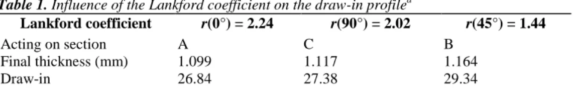
The Lankford coefficients used for the constitutive law based on a constant texture come from the black thick curve in Fig. 8. The reasoning described above leads to Table 1 for this steel and the constant texture based law. On the finite element mesh, three particular elements along the three studied directions are chosen such that they undergo completely the drawing process on the curvature of the die. The texture at the end of the deep-drawing process for the law using an evolving texture is examined for the three directions. As the Lankford coefficient has proved to be an important parameter for deep-drawing processes, it is computed for these three elements as shown in Fig. 8. Significant differences of the r values appear for the three particular directions according to the initial curve and to each other. This can explain why the draw-in profile is more pronounced if the texture is evolving during the process.
Table 1. Influence of the Lankford coefficient on the draw-in profilea
Lankford coefficient r(0°) = 2.24 r(90°) = 2.02 r(45°) = 1.44
Acting on section A C B
Final thickness (mm) 1.099 1.117 1.164
Draw-in 26.84 27.38 29.34
a The value of the Lankford coefficient decreases from columns 2 to 4 and that of the final thickness and draw-in increases from columns 2 to
4.
4. Conclusion
On the deep-drawing application presented here, the influence of the evolving texture is relatively small on the main results of the simulation. However, if we focus on the final texture and particularly on the resulting Lankford coefficients, a large difference can be noticed from one element to another and to the initial behaviour. It is then important to take into account the texture evolution of the steel sheet for each element of the mesh. This leads to computing problems: large amounts of memory storage and large computation time. Nevertheless, the simulation has been managed in 2 days with parallel computation.
Acknowledgements
As Research Associate of the National Fund for Scientific Research (Belgium), A.M. Habraken would like to thank this Belgian research fund for its support.
References
[1] L. Duchêne, Implementation of a yield locus interpolation method in the finite element code LAGAMINE, DEA Graduation Work, Ulg, Liège, Belgium, 2000.
[2] L. Duchêne, A. Godinas, A.M. Habraken, Metal plastic behaviour linked to texture analysis and FEM method, in: Proceedings of the Fourth International Conference NUMISHEET99, 1999, pp. 97-102. [3] A. Godinas, Définition locale du comportement plastique d'un matériau, Intermediate Report No. 27, Convention RW No. 2748, Région Wallonne, Ulg, Liège, Belgium, 1998.
[4] S. Munhoven, A.M. Habraken, A. Van Bael, J. Winters, Anisotropic finite element analysis based on texture, in: Proceedings of the Third International Conference NUMISHEET 96, 1996, pp. 112-119.
[5] J. Winters, Implementation of texture-based yield locus into an elastoplastic finite element code, Ph.D. Thesis, KUL, Leuven, Belgium, 1996.