ÉTUDE DE LA CIRCULATION DANS
LE BASSIN DE FOXE (CANADA)
RAPPORT PRÉSENTÉ À L'UNIVERSITÉ DU QUÉBEC À RIMOUSKI comme exigence partielle du programme
de doctorat en océanographie
PAR
MARC DEFOSSEZ
UNIVERSITÉ DU QUÉBEC À RIMOUSKI
Service de la bibliothèque
Avertissement
La diffusion de ce mémoire ou de cette thèse se fait dans le respect des droits de son
auteur, qui a signé le formulaire « Autorisation de reproduire et de diffuser un rapport,
un mémoire ou une thèse ». En signant ce formulaire, l’auteur concède à l’Université du
Québec à Rimouski une licence non exclusive d’utilisation et de publication de la totalité
ou d’une partie importante de son travail de recherche pour des fins pédagogiques et non
commerciales. Plus précisément, l’auteur autorise l’Université du Québec à Rimouski à
reproduire, diffuser, prêter, distribuer ou vendre des copies de son travail de recherche à
des fins non commerciales sur quelque support que ce soit, y compris l’Internet. Cette
licence et cette autorisation n’entraînent pas une renonciation de la part de l’auteur à ses
droits moraux ni à ses droits de propriété intellectuelle. Sauf entente contraire, l’auteur
conserve la liberté de diffuser et de commercialiser ou non ce travail dont il possède un
exemplaire.
Cette thèse a été réalisée, jusqu'à son décès, sous la direction de Monsieur François Saucier, professeur à l'Institut des sciences de la mer de Rimouski (ISMER). La codirection a été assurée par Messieurs Paul Myers, professeur associé à l'Université d'Alberta et président de la Société canadienne de météorologie et d'océanographie, et Daniel Caya, professeur associé à l'Université du Québec à Montréal et directeur de l'équipe de simulations numériques au Consortium OURANOS-UQAM. Le comité de thèse était composé des personnes précédemment citées et de Monsieur Jean-François Dumais, professeur et directeur des programmes à l'ISMER. La soutenance a eu lieu le 6 octobre 2008 à l'ISMER devant le jury d'évaluation composé de:
Monsieur Éric Hudier (président du jury), professeur à l'Université du Québec à Rimouski;
Madame Daniela Di lorio (examinatrice externe), professeur associée à l'Université de Georgia, Athens, USA;
Monsieur Jean-François Dumais (examinateur interne), professeur à l'Institut des sciences de la mer de Rimouski;
Monsieur Paul Myers (codirecteur de thèse), professeur associé à l'Université d'Alberta;
Monsieur Daniel Caya (codirecteur de thèse), professeur associé à J'Université du Québec à Montréal.
Je remercie ici toutes les personnes qui ont contribué à la réalisation de ce travail, en particulier les membres du comité de thèse ainsi que Monsieur Hudier et Madame Di Iorio pour leurs précieux commentaires qui ont permis d'améliorer le rapport final.
11
RÉSUMÉ
Le bassin de Foxe est une région mal connue du système de la baie d'Hudson, un ensemble formé de trois mers intérieures à l'extrême nord du Canada, car il est recouvert de glace plus de six mois par an et que cela le rend difficile d'accès. Il est susceptible d'être très affecté par les changements climatiques, car son océanographie dépend fortement de la formation, de la couverture et du déplacement de la glace de mer. La présente étude se propose donc d'éclairer certains aspects de la circulation dans le bassin, en particulier la circulation des eaux profondes dans le chenal de Foxe et la circulation hivernale. Elle s'appuie pour cela sur un ensemble d'observations nouvelles issues de mouillages pluriannuels, de 2003 à 2006, complétées par des simulations réalisées sur la période 200 1-2005 à l'aide d'un modèle couplé glace de mer-océan avec forçages atmosphériques. Ces données ont permis de mettre en évidence la propagation au fond du chenal d'un courant de gravité qui prend son origine dans les polynies côtières à chaleur latente de l'ouest du bassin de Foxe. Ces eaux denses renouvellent chaque année plus des deux tiers des eaux profondes dans le chenal et ont assez d'énergie pour franchir un seuil à 180 m de profondeur et déborder dans la baie d'Hudson. Le volume des eaux denses produites dans les polynies a pu être estimé en calculant les flux de chaleur à l'interface mer-atmosphère et a été trouvé égal à 1,53.1012
m3
• L'ouverture des polynies en plein hiver entraîne la synchronisation des écoulements d'eau dense, sous forme de cascade et de convection profonde. Ce phénomène est dépendant des conditions atmosphériques, donc de l'oscillation arctique, et devrait répondre au réchauffement global. L'hiver et l'été peuvent être définis par le taux de croissance de la glace de mer sur le bassin. La glace induit des changements sur la circulation générale et les marées, y compris à 150 m de profondeur. Cette glace possède aussi une dynamique très active et les courants qu'elle forme sont réguliers et forts, de l'ordre de 25 cm S'I. Même si elle pénètre parfois dans le nord-est de la baie d'Hudson, elle n'y reste pas et finit par rejoindre la Mer du Labrador via le détroit d'Hudson, sous forme solide ou fondue; le calcul indique qu'un tiers de toute la glace produite dans le bassin de Foxe est ainsi exportée. Enfin, le bilan des transferts d'eau de mer et de sel au travers d'une section en sortie du bassin montre que la circulation estuarienne de ce dernier forme un couple positif-négatif, la partie positive étant cependant perturbée par le passage du courant de gravité.
TABLE DES MATIÈRES
REMERCIEMENTS ET AV ANT-PROPOS ... 1
RÉSUMÉ ... ii
TABLE DES MATIÈRES ... iii
LISTE DES TABLEAUX ... vii
LISTE DES FIGURES ... viii LISTE DES ABBRÉVIATIONS, SIGLES ET ACRONYMES ... xi
NOMENCLATURE ... xiv
I. INTRODUCTION GENERALE ... 1
II. MULTI-YEAR OBSERVATIONS OF DEEP WATER RENEW AL IN FOXE BASIN, CANADA ... 10
ABSTRACT ... ... ... ... 1 1 II.l. INTRODUCTION ... 12 II.2. OBSERVATIONS AND METHOD ... 16
II.2.I. Oceanographie data ... 16
11.2.2. Data processing ... 17
II.3. DENSE WATER SPEED IN FOXE CHANNEL ... 28
II.3.l. Vertical propagation speed of the dense water signal ... 28
II.3.2. Ca1culation of horizontal mean speed of the dense water current ... 29
IV
IIA.l. Origin of the dense water mass detected at depth in Foxe Channel ... 31
II.4.2. Recurrence of the dense water pulse at the bottom of Foxe Channel ... 37
II.4.3. Effect of the dense water circulation on the water column in Foxe Channel 40 11.5. CONCLUSION ... 43
III.
ANAL YSIS OF A DENSE W ATER PULSE FOLLOWING MID-WINTER OPENING OF POLYNY AS IN WESTERN FOXE BASIN, CANADA ... 45ABSTRACT ... 46
III.I. INTRODUCTION ... 47
IIL2. DATA DESCRIPTION AND METHOD ... 52
111.2.1. Oceanographic and meteorological data ... 52
111.2.2. Satellite data ... 56
111.3. RESULTS ... 61
111.3.1. Heat fluxes calculations in western Foxe Basin's polynyas ... 61
111.3.1.1. Calculation for the 2003-2004 winter ... 61
III.3.1.2. Calculation for the years 1984-2006 ... 65
III.3.2. Production of dense water in western Foxe Basin's polynyas ... 69
111.3.2.1. Calculation of the produced sea-ice and rejected salt masses ... 69
lIL3.2.2. Calculation of the dense water volume ... 73
111.4. DISCUSSION ... 77
I1IA.1. Dense water production in western Foxe Basin's polynyas ... 77
IIIA.2. Consequences of the mid-winter opening of western Foxe Basin's polynyas ... 79
IlIA.3. Atmospheric pressure and synoptic scale ... 81
111.5. CONCLUSION ... 88
IV. COMPARING WINTER AND SUMMER ESTUARINE CIRCULATION IN FOXE BASIN, CANADA ... 90
ABSTRACT ... 91 IV.l. INTRODUCTION ... 92
IV.2. MODEL DESCRIPTION AND OBSERVATIONS ... 98
IV .2.1. Model ... 98
IV.2.2. Observations ... 100
IV.3. FOXE BASIN PHYSICAL OCEANOGRAPHY ... 102
IV.3.1. Winter and summer definition ... 102
IV.3.2. Sea-ice dynamics ... 102
IV.3.3. Water characteristics and mean circulation ... 109
IV.3.3.1. In winter ... 110
IV.3.3.1.). At the surface ... 110
IV.3.3.1.2. At the bottom ... 113 IV.3.3.2. In sUlnmer ... 114
IV.3.3.2.1. At the surface ... 114
IV.3.3.2.2. At the bottom ... 115
IVA. MASS TRANSFERT BETWEEN THE SURROUNDING PARTS OF FOXE BASIN ... 117
VI
IV.4.2 Ice transport ... 121
IV.5. TIDAL ANALYSIS ... 125
IV.6. DISCUSSION AND CONCLUSION ... 128
V. CONCLUSION GENERALE ... 131
LISTE DES TABLEAUX
Tableau II.I Characteristics of the T -S mixing lines at the bottom of Foxe Channel during the dense water pulse for the years 2004 and 2005 ... 25 Tableau III. 1 Main topographic elements of Foxe Basin ... 50 Tableau III.2 Main characteristics of western Foxe Basin's polynyas ... 60 Tableau III.3 Relative contribution of the sensible H; and latent H ~ heats, and of
the upwards H~wIIP and downwards H~Wd(lwll longwaves to the net heat exchanged at the polynyas' surface ... 66 Tableau III.4 Ca1culation of sea-ice mass (M ice)' rejected salt mass (M,.u't ) and
dense water volume (Vdw) produced in western Foxe Basin's
polynyas during the 2003-2004 winter ... 70 Tableau IV.I Mean speed and total distance covered by the Lagrangian tracers
leaving Foxe Basin ... 108 Tableau IV.2 Velocity and phase components vs. tidal constituents in Foxe Channel
Figure II.I Figure II.2 Figure II.3 Figure II.4 Figure II.5 Figure II.6 Figure II.7 Figure Il.8 Figure II.9
LISTE DES FIGURES
Foxe Basin and sUlTounding parts of the Hudson Bay system based on
ETOP02
...
...
...
....
...
.
...
....
...
13 Deep water seasonal cycle observed in 2004-2006 in Foxe Channel ... 18 Temperature over the last 200 m of the water column in FoxeChannel ... 20 Temporal profile of the dense water mass f10wing in Foxe Channel
... 22
Vertical propagation of the dense water signal ... 23 Comparison between the salinity at 360 and 150 m depth in Foxe Channel ... 26 T -S diagram representing the mixing of Foxe Channel' s deep waters with the incoming dense waters for 2004 and 2005 ... 27 Dense water circulation and cascade in Foxe Basin ... 34 Satellite image showing the sea-ice distribution on March 4, 2004, over western Foxe Basin ... 36 Figure III. 1 Hudson Bay system and Foxe Basin ... 48 Figurem.2
Foxe Channel's deep water response to sea surface atmosphericevents ... 53 Figure I1L3 Atmospheric parameters averaged from 1984 to 2006 at Repulse Bay
and Hall Beach weather stations ... 57 VIII
Figure IlIA Satellite images showing the opening of polynyas in western Foxe Basin ... 58 Figure III.5 Net daily integrated sea-atmosphere heat exchanges in western Foxe
Basin's polynyas ... 64 Figure 111.6 Sea-atmosphere heat exchanges averaged from 1984 to 2006 in Lyon
Inlet's polynya, in the polynya along Melville Peninsula's eastern coast, and in Hall Beach's polynya ... 68 Figure 111.7 Schematic representation of frazil ice and dense water formation
following intense heat loss at a latent heat polynya's surface ... 74 Figure 111.8 Comparison of surface air pressure in the north and south of the
Hudson Bay system ... 84 Figure 111.9 Consequence of the meridional inversion of the atmospheric pressure
in mid-winler and over the Hudson Bay system on the wind velocity field at 10 m in Foxe Basin ... 85 Figure
III.
10 Schematic representation of the incoming dense water mass at thebottom of Foxe Channel in winter and of its effects on
sedimentation ... 86 Figure IV. 1 Hudson Bay system and Foxe Basin ... 93 Figure IV.2 Simulated ice growth rate averaged over Foxe Basin ... 103 Figure IV.3 Simulted ice growth rate averaged over the winter in Foxe Basin .. lOS Figure IVA Simulated sea-ice trajectory in Foxe Basin ... 107 Figure IV.5 Simulated temperature, salinity and seawater velocity fields,
averaged over winter and summer in Foxe Basin ... III Figure IV.6 Vertical simulate seawater (a) and salt transport (b) through the cross
x
Figure IV.7 Simulated sea-ice thickness averaged over the winter in Foxe Basin 122 Figure IV.8 Satellite image taken on June 20, 2002 over Foxe Basin and its
surrounding parts ... 123 Figure V.I Comparaison entre les observations et les simulations en température et
AO BB CAA CI CLIVAR CTD DS ESA ETOP02 FB FC FDD FHS FP GB HaB HB HS
KI
LISTE DES ABBRÉVIA TIONS, SIGLES ET ACRONYMES
Arctic Oscillation Baffin Bay
Canadian Arctic Archipelago Coats Island
Climate Variability
Conductivity Temperature Depth Davis Strait
European Space Agency Earth Topography 2 minutes Foxe Basin Foxe Channel Freezing Degree Days Fury and Hec1a Strait Foxe Peninsula Gulf of Boothia Hall Beach Hudson Bay Hudson Strait
LI LS
M2
MERICA MI MPN2
NA NI NOAA 01 PCI RB RWS S2 SBS SBT SD SI SSS Lyon Inlet Labrador Seaconstituent lunaire semi-diurne de la marée Mers Intérieures du Canada
Mansel Islands Melville Peninsula
constituent lunaire elliptique semi-diurne de la marée North Atlantic
Nottingham Island
National Oceanic and Atmospheric Administration constituent lunaire déclinationnel diurne de la marée
XII
Points sur la droite de mélange avant et après le début du courant de gravité Prince Charles Island
Points sur la droite de mélange avant et après la fin du courant de gravité Repulse Bay
Roes Welcome Sound
constituent solaire semi-diurne de la marée Sea Bottom Salinity
Sea Bottom Temperature Standard Deviation Southampton Island Sea Surface Salinity
SST Sv T-S UNESCO
U
Te
WISea Surface Temperature
Sverdrup (unité: lSv == 106 m3s-l) Temperature-Salinity
numéros des Traceurs
United Nations Educational, Scientific and Cultural Organization Coordinated Universal Time
e
f
g n s u v wz
ANOMENCLA TURE
épaisseur de la glace de mer paramètre de Corio lis accélération de la gravité nombre d'annéespente topographique
composante ouest-est du vecteur courant composante sud-nord du vecteur courant vitesse de la masse d'eau dense
composante fond-surface du vecteur courant profondeur
surface d'une polynie
surface d'une section transverse du chenal de Foxe comprise entre le fond et le sommet de la masse d'eau dense
surface maximale d'une polynie active
coefficient de transfert en volume pour la chaleur latente coefficient de transfert en volume pour la chaleur sensible chaleur spécifique de l'air
à
pression constanteflux de chaleur latente
Rs L Mml,
Q
,
Q.wllS
Si S"U!Qn Tflux des ondes longues
flux des ondes longues dirigées vers le bas flux des ondes longues dirigées vers le haut flux de chaleur net
flux de chaleur sensible
chaleur latente de fusion de l'eau de mer chaleur latente de vaporisation de l'eau de mer masse de la glace de mer
masse de sel rejeté dans la colonne d'eau densité de vapeur atmosphérique
densité de vapeur à la surface de la mer débit de sel par une section
débit d'eau par une section salinité de l'eau de mer salinité des eaux denses
salinité moyenne de la glace de mer salinité moyenne dans le bassin de Foxe salinité moyenne de surface
salinité sur la section
salinité des eaux environnantes température de l'eau de mer température de l'air à 10 m
T.
,
U1-e
P
P
o
PairP
dwP
.
nv
(Jr
température des eaux denses
température de l'eau de surface dans une polynie température des eaux environnantes
composante longitudinale du courant dans le chenal de Foxe composante transversale du courant dans le chenal de Foxe volume des eaux denses produites
volume initial des eaux denses
volume des eaux environnantes servant à produire les eaux denses composante nord-ouest sud-est de la vitesse du vent à 10 m
émissivité de l'air
émissivité de la surface de la mer
déphasage de la composante M2 de la marée densité de l'eau de mer
densité de l'eau douce densité de l'air
densité des eaux denses densité de la glace de mer densité des eaux environnantes constante de Stefan-Boltzmann
temps caractéristique de résidence des eaux profondes
<l> Il phase de la composante longitudinale du courant dans le chenal de Foxe phase de la composante transversale du courant dans le chenal de Foxe
1. INTRODUCTION GENERALE
La géographie particulière du bassin de Foxe en fait un sujet très intéressant pour l'étude de la circulation dans une mer arctique-subarctique, car le bassin ne comporte qu'un plateau au nord et un chenal au sud et qu'il est bien isolé des mers voisines par des complexes formés d'îles et de seuils. Ceci donne une topographie relativement simple et
qui facilite le suivi des masses d'eau entrantes, sortantes ou s'écoulant à l'intérieur du bassin. Mais c'est cette même géographie qui est responsable du déficit en données dans la région, car l'éloignement et le climat rigoureux compliquent les campagnes de mesure,
surtout en hiver quand la glace de mer rend la navigation impossible. Ainsi, des pans entiers de l'océanographie physique du bassin de Foxe étaient jusqu'à présent négligés, en particulier la circulation des eaux profondes dans le chenal de Foxe et la circulation hivernale. Le but principal de cette thèse est donc d'apporter des réponses sur ces aspects méconnus du bassin de Foxe, mais c'est aussi de dresser un état des lieux sur sa situation actuelle afin de fournir une base pour évaluer l'impact des changements climatiques à venir.
A vant d'aborder le cœur du problème, il convient de préciser quelques éléments
géographiques sur le bassin de Foxe. Le bassin est la partie la plus septentrionale du
système de la baie d'Hudson, un ensemble composé de trois grandes mers intérieures, et il
subit à la fois les influences de l'Arctique et du continent nord américain. Son centre est assez bien défini par le point de coordonnées 66
O
N
et 800
0
,
c'est à dire que le bassin esttraversé en son mjleu par le cercle polaire arctique, ce qui a une grande incidence sur la formation des glaces à cause des flux radiatifs solaires faibles sur cette région en hiver. Ses moitiés nord et sud se distinguent surtout par la bathymétrie: la partie nord est formée à l'est par des estrans et à l'ouest par un chenal peu profond, variant d'environ 15 à 150 m et longeant sur 300 km la côte est de la péninsule de Melville, tandis que la partie sud est essentiellement formée du chenal de Foxe, long de 350 km et atteignant des profondeurs de l'ordre de 450 m. Le bassin est compris entre l'île de Baffin au nord et à l'est, l'île Southampton au sud et la péninsule de Melville à l'ouest. Il communique avec l'Arctique via le détroit de Fury et Hecla, avec la mer du Labrador via le détroit d'Hudson, et avec la baie d'Hudson via le détroit de Roes Welcome et le passage entre les îles Southampton et Nottingham. La surface du bassin est approximativement de 0,2· 1012
m2
, pour un volume
de 0,2.1014 m3
. Comparativement, la baie d'Hudson fait 0,8.1012 m2 en surface et 1,1.1014
m3
en volume, et le détroit d'Hudson 0,2.1012
m2
et 0,4.1014 m3
. Le bassin de Foxe est donc relativement "petit" vis-à-vis de ses voisins. Cependant, c'est aussi une voie par
laquelle transitent une fraction des eaux arctiques qui se rendent dans l'Atlantique Nord, augmentées au passage par l'apport flu vial et glaciel. Le bassin joue donc un rôle important dans la circulation thermohaline et cela justifie, dans le contexte des changements climatiques, le regain d'intérêt que cette région suscite depuis quelques années.
L'aspect le mOins bien connu de la circulation dans le bassin de Foxe est certainement la circulation des eaux profondes dans le chenal de Foxe. En effet, il aura fallu attendre l'année 2003 pour que des mouillages y soient déployés dans le cadre des missions
3
pluriannuelles MERICA (Saucier et al., 2004b). Les séries temporelles obtenues permettent désormais de suivre sans interruption l'évolution saisonnière des propriétés des eaux profondes dans le chenal. Auparavant, il n'existait que des mesures sur quelques stations, réalisées lors de campagnes océanographiques estivales. Les données de ces campagnes, assez anciennes et rares de surcroît, n'ont pas permis de fournir une description précise de la circulation profonde, même si la présence d'eau très froide
«
-1,80 oC) et salée (> 33,75) dans le chenal de Foxe a été attestée dès 1955 par Campbell (1964), et de nouveau en 1982 par Jones et Anderson (1994). Comme ces auteurs ne disposaient que d'observations éparses, tant spatialement que temporellement, ils n'ont pu que conjecturer sur la formation et la circulation de ces eaux denses, sans jamais pouvoir valider leurs scénarios. Ces lacunes dans la connaissance de l'océanographie du bassin de Foxe en ont engendré d'autres. Par exemple, des mesures en alcalinité et en carbonates ont montré qu'une partie des eaux profondes du chenal de Foxe déborde dans la baie d'Hudson (Jones et Anderson,1994), mais il n'a pas été alors possible de quantifier ce phénomène.
Le premier objectif de cette thèse est donc d'améliorer la compréhension de la circulation profonde dans le chenal de Foxe. L'accent est mis principalement sur le renouvellement des eaux profondes afin d'en estimer l'ampleur ainsi que la variabilité interannuelle. Cette question est importante, non seu lement parce qu'elle permet de mieux décrire la circulation dans le bassin de Foxe, mais aussi parce qu'elle conditionne la ventilation en oxygène et donc la biologie au fond du chenal. La recherche de l'origine des eaux profondes ainsi que les conséquences de leur circulation sur la colonne d'eau sont
incluses dans cet objectif.
La méthode employée pour réaliser cette première étude repose principalement sur les observations en température et en salinité issues des mouillages MERICA 2003 à 2006 acquises du bas de la colonne d'eau (150 m) jusqu'au fond du chenal (360 ou 440 m, selon le mouillage). Ces trois années successives de données permettent d'étudier la récurrence et la variabilité des phénomènes saisonniers. Des données simulées issues du modèle
numérique développé par Saucier et al. (2004a) sont aussi utilisées pour rechercher l'origine des eaux denses du bassin de Foxe à l'aide de traceurs lagrangiens, selon une procédure de pistage à rebours.
Une des particularités des mers polaires est que ce sont des régions qui produisent des quantités importantes d'eau froide riche en saumure lors du gel des eaux salées de surface. Ainsi, dans l'Arctique, elles contribuent à la maintenance de la couche supérieure de l'halocline, ce qui a des conséquences sur la circulation thermohaline dans l'Atlantique Nord. Aagaard et al. (1981) ont estimé que l'ensemble des plateaux arctiques produisaient environ 2,5 Sv (1 Sv == 106 m3s-') d'eau dense; quant à Cavalieri et Martin (1994), ils ont calculé que la contribution des polynies côtières arctiques était comprise entre 0,7 et 1,2 Sv. Dans le cas du bassin de Foxe, les résultats du premier objectif montrent (voir chapitre II) que les eaux denses détectées au fond du chenal de Foxe se forment dans les polynies côtières à chaleur latente de l'ouest du bassin, et qu'elles se propagent ensuite comme un courant de gravité dans le chenal. Le problème qui se pose alors naturellement est de
5
vérifier que, d'une part, la production d'eau dense dans les polynies suffit à expliquer le
renouvellement des eaux profondes et que, d'autre part, la chronologie des différents
évènements est compatible avec ce scénario.
Le second objectif complète donc le prernier en fournissant une analyse quantitative des mécanismes menant à la propagation le long du chenal de Foxe de la masse d'eau dense
trouvant son origine dans les polynies de l'ouest du bassin de Foxe. Ceci revient essentiellement à calculer les flux de chaleur entre la surface de la mer et l'atmosphère au niveau des polynies puis à en déduire les quantités de glace et d'eau dense produites.
L'intérêt de ce type d'analyse ne fait aucun doute, car les paramètres de ces calculs dépendent fortement des conditions météorologiques présentes en hiver au dessus du bassin
et il est donc probable que les changements climatiques tels qu'anticipés par les modèles numériques (Johns et al., 1997; Emori et al., 1999) affecteront sensiblement les résultats
actuels. Ce deuxième objectif est complété par une discussion sur le lien probable entre
l'intensité de la production d'eau dense dans les polynies et l'index de l'oscillation arctique, ce qui permet d'étendre la portée de cette recherche au-delà du seul cadre du
bassin de Foxe.
Les calculs des flux de chaleur pour cette seconde étude nécessitent la connaissance
de la dynamique spatiale des polynies qui est déterminée ici à l'aide d'images satellites montrant leur ouverture au milieu de l'hiver. Ils nécessitent aussi la connaissance des vents et de la température de l'air qui sont obtenus à partir des enregistrements de deux stations
météorologiques situées au nord-ouest du bassin de Foxe (à Hall Beach) et au sud-ouest (à Repulse Bay). Ces mesures proviennent des bases de données d'Environnement Canada,
elles ont été acquises toutes les heures à l'altitude de 10 m; dans cette thèse, elles ont en plus été extrapolées à midi chaque jour (cette extrapolation a été rendue nécessaire à cause des données manquantes). Les calculs de flux sont réalisés pour l'hiver 2003-2004, car, dans le bassin, cette année peut être considérée comme standard du point de vue météorologique. De plus, ces calculs sont généralisés à l'aide d'une quasi-climatologie sur
21 ans consistant à moyenner les données, à partir du 1 er janvier de chaque année, et
couvrant la période 1984-2006.
Les premier et second objectifs définis aux paragraphes précédents se concentrent principalement sur le renouvellement des eaux profondes du bassin de Foxe. Bien que cela soit indispensable pour comprendre la circulation dans le bassin, et même si cela peut donner des informations sur les débordements d'eau dense du bassin vers la baie d'Hudson,
cela ne suffit pas à décrire la circulation générale ni les échanges avec les mers voisines. Il
est donc nécessaire de compléter cette thèse avec une description des courants et de la
répartition en température et salinité à l'échelle du bassin de Foxe dans son ensemble. Des travaux antérieurs (Prinsenberg, 1986; Saucier et al., 2004a) ont signalé que la circulation
dans le bassin était estuarienne, c'est à dire gouvernée par les gradients de densité entre les
masses d'eau douce jouxtant les masses d'eau salée. Mais ces travaux restent assez vagues
en ce qui concerne le type de circulation estuarienne, bien que Prinsenberg (1986) ait
7
estuaire négatif en hiver et positif en été. De plus, ces travaux se contentent généralement
d'indiquer que les courants sont affaiblis et que parfois leur sens s'inverse en hiver. Pourtant, l'action de la couverture de glace ne se limite pas à réduire les échanges de chaleur à l'interface mer-atmosphère ni à ajouter de la friction et de l'amortissement à
l'interface mer-glace: elle retire aussi des quantités non négligeables d'eau douce à la surface de la mer lorsqu'elle se forme. Or, ce dernier point est loin d'être anecdotique, car, ainsi que l'ont montré El-Sabh et al. (1997), les zones côtières des mers polaires sont
susceptibles de connaître une circulation estuarienne négative quand l'extraction d'eau douce en surface par formation de glace excède l'apport dû au ruissellement. Ce phénomène peut modifier profondément les flux de matière et mérite d'être étudié de
manière approfondie. De plus, MacDonald (2000) a aussi introduit la notion de couple
positif-négatif pour les estuaires à haute latitude, en insistant sur la sensibilité de ces couples aux variations climatiques.
Le troisième objectif de cette thèse est donc double: d'une part fournir une description aussi précise que possible de la circulation générale dans le bassin de Foxe, ce
qui inclut la circulation de la glace de mer, et d'autre part caractériser le type de circulation estuarienne du bassin afin de voir si elle forme un couple positif-négatif. Une étude à
profondeur moyenne (150 m) dans le chenal de Foxe est aussi fournie pour déterminer l'influence du couvert de glace sur les courants de marée; l'étude en surface ayant déjà été réalisée par Saucier et al. (2004a).
La description et la caractérisation de la circulation dans le bassin de Foxe reposent entièrement sur le modèle numérique développé et décrit en détail par Saucier et al.
(2004a). Ce modèle baroclinique donne des résultats très réalistes dans les mers côtières peu profondes et reproduit particulièrement bien les phénomènes à mésoéchelle. C'est donc un très bon outil pour cette troisième étude, car les simulations permettent d'obtenir des données en température, en salinité, en courant et sur les caractéristiques (épaisseur, taux de croissance-fonte, vitesse) de la glace de mer en tout point du bassin et à tout instant sur la période 2001 à 2005. II faut noter que bien que le pas de temps interne du modèle soit de cinq minutes, les sorties sont moyennées ici sur trois heures pour limiter la taille des fichiers résultats. Ceci est amplement suffisant pour obtenir une bonne précision dans les calculs puisque cette période inclut les principaux constituants de la marée qui est essentiellement de type semi-diurne dans le bassin. En considérant que le passage entre la pointe est de l'île Southampton et la pointe ouest de la péninsule de Foxe sépare le bassin de Foxe à la fois de la baie d'Hudson et du détroit d'Hudson, ce qui revient à "court-circuiter" l'île Nottingham, il n'existe alors que trois voies d'accès au bassin: par les détroits de Fury et Hecla et de Roes Welcome, et par le passage décrit ci-dessus. Les deux premières voies représentent des entrées du bassin, c'est à dire que le transport d'eau en moyenne annuelle se fait vers le bassin, donc la troisième est nécessairement une sortie. C'est pourquoi c'est au niveau de cette dernière qu'est définie la section sur laquelle sont effectués les calculs de transfert de masse d'eau. L'analyse harmonique des marées à mi-profondeur dans le chenal de Foxe est réalisée non pas avec des données simulées, qui sont bien adaptées aux calculs de moyennes sur des portions de la grille numérique, mais plutôt avec des mesures en
9
courant issues de la campagne MERICA 2005, car ces observations permettent d'obtenir
une meilleure précision en un point unique.
Le premier objectif est développé dans le Chapitre II qui a fait l'objet d'un article scientifique publié en 2008 dans la revue Atmosphere-Ocean, sous le titre: "Multi-year
observations of deep water renewal in Foxe Basin, Canada". Le second objectif est développé dans le Chapitre III; il fait lui aussi l'objet d'un article qui a été accepté avec corrections mineures dans la revue Dynamics of Atmospheres and Oceans, sous le titre: "Analysis of a dense water pulse following mid-winter opening of polynyas in western Foxe Basin, Canada". Quant au troisième objectif, il est développé dans le Chapitre IV qui est également écrit sous la forme d'un article; il est prévu qu'il soit soumis à une revue spécialisée en modélisation océanographique physique sous le titre: "Comparing winter
and summer estuarine circulation in Foxe Basin, Canada". Toutes les revues dans
lesquelles ces articles sont ou seront publiés sont internationales et à comité de lecture. La conclusion générale de cette thèse est donnée dans le Chapitre V qui résume les principaux
II. MULTI-YEAR OBSERVATIONS OF DEEP WATER RENEW AL IN FOXE BASIN, CANADA
Il
ABSTRACT
New oceanographie mooring data recorded between 2004 and 2006 show each year an abrupt arrivaI of cold and saline water at the bottom of Foxe Channel. Foxe Channel is
the deepest part of Foxe Basin, an arctic/subarctic inland sea in the Hudson Bay system.
This dense water mass is detected at depth in the middle of the channel at the beginning of spring. It is characterized by a sharp temperature drop and salinity rise. This pulse-like phenomenon is recurrent, although there is sorne interannual variability depending on the severity of the preceding winter. The dense water probably originates from western Foxe
Basin' s coastal polynyas. A gravit y current in Foxe Channel f10ws southeastwards and significantly modifies the water column along the channel by raising the isotherms by
140 m. The water column responds to the dense water pulse with a time lag of one month.
Although the pulse lasts only three months, it renews more than 2/3rd of the deep waters in
Foxe Channel and is therefore an important component of Foxe Basin general circulation. This shows that the pulse is an energetic event and that the newly advected dense waters
II.1. INTRODUCTION
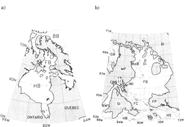
Foxe Basin (FB) is an inland sea included in the Hudson Bay (HB) system, Canada (Fig. II.I). The basin is weil delimited from the other regions of the system either by sills or constrictions that control and limit deep water circulation. FB may be divided into four
parts, the three largest are: a) a wide and less than 50 m deep shelf starting from the tip of Foxe Peninsula (FP) and covering the eastern and northern parts of the basin; b) a shallow, widening and gently sloped channel reaching 100 m depth along Melville Peninsula (MP) in the western part; and c) Foxe Channel (FC), a channel 400 km long and 100 km wide reaching depths of 450 m. The fourth, smaller and off-center part of FB is called Repulse
Bay (RB) which is a depression reaching 200 m depth, located in southwest FB where it connects to HB via Roes Welcome Sound (RWS).
Arctic water coming from the Gulf of Boothia (GB) enters FB through Fury and Hecla Strait (FHS) where it is weil mixed by currents and tides (Sadler, 1982; Godin and Candela, 1987); the estimated transport is 0.04 Sv (1 Sv
=
106 m3s-l) in winter (Sadler,1982) and 0.1 Sv in summer (Barber, 1965). This arctic water is less dense than the waters of FB and tends to tlow at the surface (Prinsenberg, 1986). FB is an important contributor
to the general circulation in the HB system: in summer, freshwater due to runoff and ice
melting is exported by surface currents from FB to the other parts of the HB system while denser water enters the basin underneath and, in winter, some of FB's deep waters overtlow
13
a) b)
lIN
--- .-_ .. ' ;~,
Fig. II.l. Foxe Basin Ca) and surrounding parts Cb) of the Hudson Bay system based on ETOP02 CEarth Topography 2-minutes, NOAA). The locations of the moorings are shown with black stars. BB stands for Baffin Bay, FB for Foxe Basin, FC for Foxe Channel, FHS for Fury and Hecla Strait, FP for Foxe Peninsula, GB for Gulf of Boothia, HaB for Hall Beach, HB for Hudson Bay, HS for Hudson Strait, LI for Lyon Inlet, MP for Melville Peninsula, NI for Nottingham Island, RB for Repulse Bay, RWS for Roes WeIcome Sound, SI for Southampton Island, and WI for Winter Island.
Jones and Anderson, 1994; Ingram and Prinsenberg, 1998; Saucier et al., 2004a). However, the particulars of this circulation are poorly known, especially the dense water component, because FB is a remote region subject to severe climatic conditions. The eight-month long nearly complete sea-ice coyer over the basin explains the lack of wintertime data.
Until 2003, there were no year-Iong time series of measurable physical quantities in
FB except in the northwestern corner of the basin for the year 1955-1956 (Grainger, 1959). The few available data come mainly from oceanographic surveys made in 1955 and 1956
(Campbell, 1964) and in 1982 (Jones and Anderson, 1994; Tan and Strain, 1996). Therefore, publications about FB are scarce; Prinsenberg (1986) gives the most
comprehensive review to date of FB's physical oceanographic aspects.
In 1955 and to a lesser extent in 1956, Campbell (1964) found a cold and saline water mass at depth in Fe. This occurrence is described as a cascade of dense water by
Ivanov et al. (2004). Saucier et al. (2004a), with the help of a numerical model, reports also the renewal of deep waters at depth over 300 m in Fe. These findings, however, are not supported by year-Iong observations in temperature and salinity which are needed to
characterize this dense water mass and its associated currents.
The goal of this paper is to investigate the deep water renewal and interannual
variability at the bottom of FB. It uses new data coming from three oceanographic
moorings deployed from 2003 to 2006 at depth in Fe. The details of the moorings and data
are given in Section II.2. In these observations and for the first time, the abrupt arrivaI of a dense water mass has been detected each year in the channel. The main characteristics of
15
its consequences on the deep water renewal and over the water column in Fe are discussed
II.2. OBSERVATIONS AND METHOD
II.2.1. Oceanographie data
The oceanographie data used in this study come from three moonngs that were deployed through the pro gram MERICA (MERs Intérieures du CAnada, Saucier et al., 2004b), northern component, funded by the Oepartment of Fisheries and Oceans, Canada.
This research program started in 2003; it involves the long term monitoring of the climate variability and biological productivity of the HB system.
The ftrst mooring consisted of a CTO (Conductivity Temperature Oepth, SBE-19 from Sea-Bird Electronics) deployed at the bottom of FC from August 2003 to August 2004 at 440 m depth. Its position indicated by M8 in Fig. II. 1 a was 65.14 oN and 81.34 °W,
which corresponds to FC's deepest trough. The sampling rate of salinity, temperature and
depth was set to 15 minutes. The precision and resolution of the sensors are, respectively,
10-3 Sm-! and 10-4 Sm-! in conductivity, 10-2 oC and 10-3 oC in temperature, and 1.0 dbar
and 0.1 dbar in pressure.
The second and third moorings (M25a. b in Fig. II. 1 a) were equipped with the same CTO model (Sea-Bird SBE-19) than at M8. M25a was deployed from August 2004 to
August 2005 and M25b from September 2005 to September 2006. They were both moored at 360 m depth at the bottom of FC and their position was 64.37 oN and 80.55 °W. The
sampling rate of M25a. bIS CTO sensors was set to 30 minutes with the same sensors'
17
Additionally, Mooring M25a had temperature sensors (Mini log 12: VEMCO -AMIRIX Systems Inc.) distributed from the depth of 357 to 155 m. These devices have a
precision of 0.1 oC with a resolution of 0.015 oC, and their sampling rate was set to one
hour. This paper also uses the salinity data sampled every hour by the conductivity sensor
of a current meter (S4 from InterOcean Systems Inc.) deployed at ISO m depth at M25a.
The nominal precision and resolution in conductivity of InterOcean's S4 are 2·\0-4 Sm-! and \0-4 Sm-!, respectively.
II.2.2. Data processing
In Fig. II.2, the temperature and salinity time series from moorings M8 and M25a. b
are plotted on the same graph in order to show the continuity from one year to another of
the properties of deep water masses in Fe. It is important to note that M8 and M25a. b are
93 km apart and that they are almost aligned with Fe. The vertical dashed line in Fig. II.2
marks the gap between the moorings. This configuration has proved itself useful when
following the dense water signal flowing along the channel. In Fig. II.2a, the freezing point
curve has been caIculated according to the depth of each mooring using Millero and
Leung's formula (1976). When the freezing point is computed at the surface instead of the
mooring's depth, it matches weil with the portion of the temperature curve corresponding to
the passing of the cold water mass (T ::; -1.8 oC) for the years 2004 and 2005. This strongly
suggests that the freezing waters found at depth in FC are the result of ice formation at the
a) b) l '
l-175
0~
,~
!
,A
.... 1 1 Qi l , CL , E : Qi ] -2 c . 00l
Qi o CL , ~ freezing point :: ... _ _--W'"---._._ ... _-
'
---
'*'--
:
1 : -2.25 ' , , ( .?: :.§ o 33.5 Vl 33.0 04/01 05/01 06/01 , , 1 1 1 1 1 1 1 1 1 1 Time (yr/mo)~
:
1~~
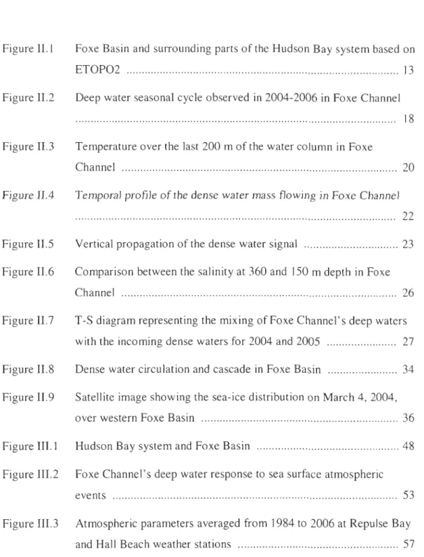
1 1 J J , J" -'.-1.---' J ,l, J J, 1 • 1 _1.1.1 _ J , J I . -l. 04/01 05/01 06/01 Time (yr/mo) 28.0 (j) <0 3 27.5 0 1 CI) " 27.0 <0 3 1 '" 26.5 ~Fig. n.2. Deep water seasonal cycle observed in 2004-2006 in Foxe Channel. Moorings M8
(2004) and M25 (2005 and 2006) data are separated by the dashed liner The thick (thin)
lines on a and b represent the temperature (freezing point) and the salinity (sigma-a) time series, respectively, On a, the double arrow shows the gap for the year 2006 between the
fragment of curve of the freezing point calculated at the sea surface and the cold waters during the pulse, The break in the freezing point curve on a is due to the 80 m difference of depth between M8 and M25.
19
In 2006, the match between the temperature curve and the freezing point at the surface is
Jess obvious since there is a gap of 0.07
o
c.
Only the part from June to August 2006 of thefreezing point at the surface is drawn in Fig. II.2a for comparison with the temperature
curve. Since the 2006 dense waters are Iikely produced by a similar freezing process than in
2004 and 2005, the gap is probably due to some additional mixing with the surrounding
waters. In Fig. 2b, the UNESCO (1981, 1983) algorithms for the sea water density and
potential temperature have been used to ca1culate the sigma-8 curve. The high frequency
component of the recorded signal being weak compared to the main seasonal signal, it was not deemed necessary to filter the data in Fig. II.2 to remove tidal effects.
In Fig. II.3, the temperature data from 155 m to the bottom of FC have been l
ow-pass filtered by a fourth order ButterwOlth filter with a cutoff period equal to 25 hours. This filtering is needed because the original time series, especially the data above 300 m depth,
are more affected by the tides as the depth decreases; in other words, the filtering of the time series below 300 m depth does not effectively alter the original data. Note that this
same filter is used throughout the paper for the other data. In Fig. II.3a, the interval in depth between each time series is equal to 12 m except for the last two sensors (l65 and 155 m)
which are 10 m apart. In order to ensure that ail curves are on the same baseline, the first
25 hours of each time series have been averaged and the result displayed above each curve at the initial time (September 14,2004). Fig. II.3b corresponds to three vertical temperature profiles taken just before (average from April 19 to 20, 2005), during (average from April 23 to 24, 2005) and after (average from May 25 to 26, 2005) the pulse-like arrivaI of dense
a) b) 160 ~ZL _______________ ~~ ______ _ ~~ --~---~~--- ~~---~~--- ~~---~---~ZL ______________ --U ________ _ ~~ __________ - - - ---u ____ ~ __ _ .a----1 $' peo k M A M A 2005 160 .J(' :_ .)\'. _ .x·· _ 200 ~. ... :,' .~
..
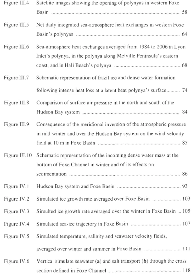
~ i ~ 240 <. 280 ~. ~ ~' 320 • ~ 360 -2.0 :x ,~ .. ' " ~. v' -1.8 ; -1.6 -1.4 -1.2 -1.0 -emperofure (oC)Fig. II.3. Temperature over the last 200 m of the water column in Foxe Channel. Ali data are low-pass filtered. The temperature at the start of each times series on a gives the
baseline while the scale is shown in the upper right of the figure. The arrow on a indicates
the first peak used to estimate the vertical propagation time and speed. The profiles in
temperature on b are drawn for the periods averaged between April 19-20 (triangles, plain
21
water in the channel.
From the data in Fig. II.3a, it is possible to reconstruct the time evolving profile of
the dense water front at the bottom of FC. This is shown in Fig. IIA by using a mask discriminating ail temperatures above -1.8
o
c.
The dashed line represents a second arder polynomial fit to visualize the profile, so that depth=
-0.038 dal -2.391 day + 362.742 and 357 m:S; depth :s; 225 m. Note that if the speed of the front is considered approximately constant, then multiplying the time coordinates of Fig. IIA's data by this speed would givethe actual spatial shape of the front. AIso, Fig. lIA suggests that the wedge formed by the
new dense waters has a height of 140 m. This height is greater than the difference in depth
between the moorings M8 and M25a. b (440 - 360
=
80 m) and legitimates the presentationof temperature and sali nit y time series on the same graph (Fig. II.2), since M8 and M25a. b
see the same deep water masses.
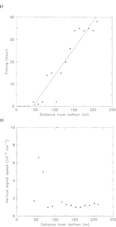
Fig. II.3a's time series are also useful to estimate the vertical propagation time and
speed of the dense water signal, which are shown in Fig. ILS. In particular, the small peak seen just after the temperature drop in Fig. II.3a, which is probably due to the adjustment of
the water colurnn caused by the passing of the dense water mass, can be used for each time series because its pattern is easy to identify. For example, this peak occurs on April 28, 2005 at 01 h UTC (Coordinated Universal Time) for the time series at 357 m depth and on
April 29, 2005 at 15 h UTC for the one at 155 m. The reference time used for Fig. II.5a
corresponds to the peak detected at 357 m depth while, in Fig. II.5b, the vertical propagation speed is calculated from the temperature sensor at the depth of 321 m in order to take into account the thickness of the dense water front.
1 160 -200 T > - 1.8°C 0
--S
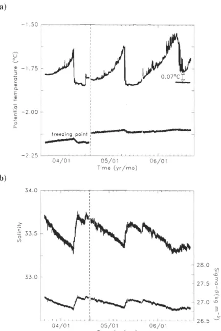
240 1- .·'0 ..c .. ··0 ~ 0.- r- .. '0 Q) 0 0 280 0 O •• ' T < -1.8°C 320 0 r- <? •.. 360 '0 0 1 0 20 30 40 Days since April 20, 2005Fig. lIA. Temporal profile of the dense water mass f10wing in Foxe Channel. The detection at the bottom of the channel of this water mass gives the reference time (to
=
0 day) of the plot. For a given depth, the point corresponds to the number of days after to from the timethe temperature falls below -1.8
oc.
The dashed line is a second order polynomial fit of the points; it separates the old deep waters (T > -1.8 oC, left of the line) from the new advancing dense waters (T < -1.8 oC, right of the line).a) b)
:
r
'--
,
c E 10-.
•.
x.
x:' o ~~~~ __ ~ __ - L _ _ - L _ _ ~ _ _ J -__ ~ __ ~~ '(1) 8 E "' , o -~ 6 1) ID Cl) Q. Vl ~ 4 Dl (1) o u "-Cl) > 2 0 o 0 50 100 150 200 250Distance from bottom (m)
x x x
x x x x
x
50 100 150 200 250
Distance from bottom (m)
23
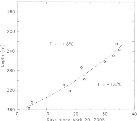
Fig. 11.5. Vertical propagation of the dense water signal. a hours smce first dense water
signal detection; b dense water signal propagation speed (see Section II.2.2 for details on the caJculation).
In Fig. II.6, the salinity time series at 150 m depth for the year 2004-2005 is drawn along the one at 360 m for comparison. Although it has been low-pass filtered in order to remove tidal frequencies, it shows more variability than the unfiltered curve at 360 m. This may be due to the influence of the HB intermediate water flowing into FC (e.g., Jones and
Anderson, 1994), although local vertical and lateral cUlTents in the channel could also play a raIe here.
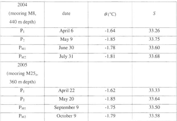
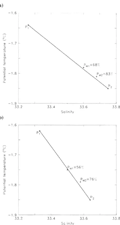
The T-S diagram in Fig. II.7 is used to estimate the percentage of mixing when the deep waters in FC are renewed by the new dense waters associated to the pulse. The temperature and salinity at the two end points PI and P2 of the rnixing line come from
Fig. 11.2. Pl represents FC's deep water characteristics just before the abrupt temperature
drop and salinity rise, while P2 represents the incoming dense water characteristics. PMI and
PM2 cOlTespond to the mixing of the deep waters at the end of the pulse and one month
later, respectively. Note that PM2 is measured before any autumn storm may disrupt the
water column in FB. The coordinates for PI, P2, PMI and PM2 are summarized in Table 11.1.
Note also that at the bottom of FC, the difference between the temperature T and the potential temperature Bis always smaller than 0.01 oC; for example, with
T
=
-1.84 oC and S=
33.75 at 440 m,B=
-1.85 oc. Despite this small difference, the temperature data have been converted to potential temperature when possible, i.e. in Fig. II.2a, II.7 and Table 11.1. In Fig. II.3 and lIA, the temperature has not been converted since there is no salinity data available at the depth of the sensors.1 25 2004 (mooring M8, date () (oC) S 440 m depth) PI April 6 -1.64 1 33.26 P2 May9 -1.85 33.75 PMI June 30 -1.78 33.60 PM2 July 31 -1.81 33.68 2005 [ (mooring M25a, 360 m depth) PI April 22 -1.62 33.33 P2 May 20 -1.85 33.64 PMI September 9 -1.75 33.50 PM2 October 9 -1.79 33.58
Table II.l. Characteristics of the T -S mixing lines at the bottom of Foxe Channel during the
dense water pulse for the years 2004 and 2005. PI and P2 are the end points of the lines. PMI
c 33 o tn z=360m A SO N D J F M A M J J A
2004
2005
Fig. II.6. Comparison between the salinity at 360 and 150 m depth in Foxe Channel. The time series at 360 m uses the original data because their high frequency component is weak compared to the seasonal cycle while the one at 150 m is low-pass filtered in order to remove the tidal signal.
27 a) - 1.6 1- Pl U 0 CIl - 1.7 1-.... 1 ~ 2 CIl Q. E
-
J
l' !Ml=68?o 0 ë !M2=83?; CIl 0 Cl.. P2 -1.9 33.2 33.4 33.6 33.8 Salinity b) -1.6 Pl u 0 ~ ~ -1.7 :l 2 CIl PM1 =56% Q. E l' 0 !M2=76% c - 1.8 CIl 0 ~ P2 -1.9 33.2 33.4 33.6 33.8 SalinityFig. II.7. T-S diagram representing the mixing of Foxe Channel's deep waters with the incoming dense waters for 2004 (a) and 2005 (b). PI and P2 are the deep water and new
dense water characteristics, respectively. PMI corresponds to the end of the dense water
arrivaI while PM2 i mea ured one month later; the numbers beside represent the percent age
II.3. DENSE WATER SPEED IN FOXE CHANNEL
Il.3.1. Vertical propagation speed of the dense water signal
In order to understand the effect of the dense water pulse over the water column, it
is useful to estimate the vertical propagation speed by detecting the signal emerging From
the pulse at different depths. These quantities are taken and ca1culated From the temperature
time series in Fig. II.3a; the results for the signal detection curve and the vertical
propagation speed are shown in Fig. II.5a and b, respectively.
In Fig. II.5a, the arrivaI time of dense water increases nearly linearly. The
regression line obtained From the least square method is: t = 0.24 d - 10.55, where t is the
detection time in hours and d is the distance in met ers From the top of the dense water layer
when the signal is first detected; the correlation coefficient for this regression is r2
=
0.89.
Note that the top of the dense water layer is used instead of FC's bottom because the peak
after the temperature drop for the series at 357, 345 and 333 m depth occurs at the same
time (April 28,2005 at 01 h UTC).
In Fig. II.5b, the vertical propagation speed is calculated as the ratio of the distance
From the top of the dense water layer divided by the travel time of the signal. This
ca1culation is in fact a time derivative that is sensitive to small inaccuracies in the data. For
that reason, the values greater than 2.10-3 ms-1 are excluded and the mean vertical
propagation speed of the dense water signal is (1.25 ± 0.22).10-3 ms-1 (it would be
29
mistaken for the thickening speed of the dense water layer which can be deduced from Fig. II.4: 140 m /26 days :::::; 5.4·] 0-5 ms-I
• In other words, although the signal can be
detected at the surface of Fe at M25's position in Jess than 4 days (360 m / 1.24.10-3 ms-I
),
it takes at least 26 days to displace the isotherms 140 m towards the surface.
II.3.2. Calculation of horizontal mean speed of the dense water current
Fig. II.3a shows that there is a cold water mass lasting from February to March
2005 and above 180 m depth in Fe. This cooling is coupled with an increase in salinity starting in February 2005 (Fig. n.6). These salt y waters are probably due to the formation of ice and associated brine rejection in FB during winter. Since this cold surface layer never
reaches the bottom of Fe and the dense water signal propagates upwards, the dense water
arrivaI in the channel may not result from a local deepening of the winter surface layer.
Furthermore, Fig. II.2 shows that the dense water pulse is detected sooner in the year at
mooring M8 (April 5) than at M25a. b (April 22 in 2005 and May 22 in 2006), M25a. b being
located 93 km southeast of M8. The time lag between the pulse detection at M8 and M25a. b
is large enough to indicate that the dense water mass travels from the northeast of Fe toward the southwest. This is coherent with the continuity of the deep water temperature and salinity (Fig. II.2a and b) seen at the beginning of August 2005. AIso, the direction of
this dense water circulation is in agreement with FC's mean cyclonic circulation. Therefore,
the dense water pulse cornes from a lateral advection of a water mass flowing southeastwards at the bottom of Fe.
water current in FC, it is interesting to have at least an estimation of its horizontal speed.
Kampfs (2000) semi-empirical approximation of dense water along-slope velocity, which
is valid for constant bottom slopes, provides a simple way to estimate this current:
- 0
25
P
d
...
-
P
III" g SIl ::::: .
dll"
f
P.nIO
(1)
where Pd,,· is the dense water density, P."," is the surrounding water density, g is the gravit y
acceleration, s is the topographic slope andfthe Coriolis parameter.
The characteri tics of the dense water produced in FB can be obtained From Fig. II.2 by taking the minimum of potential temperature and maximum of salinity at 440 m during the pulse,
i
.e
.
:
Td\\"=-1.85 oC and Sd" = 33.75 and therefore Pd\\"= 1029.28 kg.m-3. Fig. II.2gives also the characteristics of the surrounding water at the bottom of FC:
T.
n
t
=
-1.64 oC,SnI"
=
33.27 and Ps,,·=
1028.88 kg.m-3. The slope at the bottom of FC's deepest trough is s :::::: 2.4.10-3. The Coriolis parameter at the latitude of65.14 oNi
sf
= 1.
32·1O-4s-l. With these
values, Eq. 1 gives vell\"
=
1.7.10-2 mÇI .Note that this horizontal speed may be underestimated since the measurements and
ca1culations are made in a trough,
i.e.
at a location where the topographic slope flattens.According to Ivanov et al. (2004), the dense water current in the channel is the result of a
cascade. Due to the bathymetry, this cascade is likely to occur at the topographic break near
Winter Island (WI), in southwestern Fe.
In
this area, the value of the lope is 5.10-3, whichmeans that the maximal speed of the dense water CUITent would be 3.6.10-2 ms-I
31
II.4. DISCUSSION
II.4.1. Origin of the dense water
mass
detected at depth in Foxe ChannelThe characteristics of the deep waters observed in 2004, 2005 and 2006 are similar
to those reported in 1982 by Jones and Anderson (1994) who assume that they are unlikely to be renewed each year because they are trapped into the channel's depressions. However,
the observation of the dense water pulse clearly contradicts this assumption. This raises the
question about the origin of these waters: were they advected from the surrounding parts of
FB or formed in the basin?
There are three possible pathways for a water mass to enter FB (see Fig. II.l a for
locations): a) from the GB and flowing through FHS; b) from HS and passing through the
complex formed by three small islands (Nottingham (NI), Salisbury Island and Military
Island) and sills around 200 m depth; and c) from HB and overflowing either the sill at
180 m depth between Southampton Island (SI) and NI or the one at 50 m at northern RWS.
S inee the arctic waters entering FB via FHS are less dense than the waters already present
in the basin (Prinsenberg, 1986), the first hypothesis a) can be discarded and if arctic water
is found at depth in Fe, it must be through an in-situ convective proeess. Hypotheses b) and
c) are quite similar because the y both imply that dense water would have to flow over sills
smaller than 200 m deep. However, they are not consistent with the description of the
general circulation and density distribution given by Saucier et al. (2004a) and so
There are also three possibilities for in-situ dense water formation: d) concentration of brine-rich sea water repeatedly exposed to very cold winter air temperature
«
-35 oC) in eastern FB's tidal f1ats (Campbell, 1964); e) continuous brine rejection during the freezing of FB over the whole domain and sinking of the winter surface layer down to FC's bottom; and f) intense brine rejection and dense water production in western FB 's latent heat coastalpolynyas. Campbell's description seems plausible, however, neither the current nor the volume of dense water produced on the tidal f1ats can be large. In particular, the se waters are likely to be trapped in ponds and their circulation impeded by fast ice close to the sea
bottom. Furthermore, they would have to travel 700-800 km, according to FB's cyc\onic circulation, without loosing density through mixing with surrounding waters in order to
reach FC's deepest depression. Since the maximum current values estimated at depth in FB are generally less than 10-1 ms·1 (Saucier et al., 2004a), this means that the dense waters
should have been produced more than three months before reaching the trough at the
beginning of April, i.e. before the start of winter or during early winter, which is quite
improbable and thus hypothesis d) is rejected. Hypothesis e) cannot be retained either
because the continuous brine rejection during the freezing of FB is a progressive process
that is not consistent with the pulse-like propagation of the dense water signal. This would only lead to the deepening of the winter surface layer, though not enough to reach the bottom ofFC (see Section II.3.2). Therefore, the only hypothesis left is f) and the following
paragraphs are meant to further investigate its validity.
The pattern of the temperature and salinity time series in Fig. II.2 shows that the characteristics of the incoming dense waters distinguish them weil from the surroundings
33
waters. This observation can be exploited in order to attempt to trace the origin of the dense
waters by using a simple backtracking procedure and the CUITent field obtained from a
numerical mode!. The detailed description of the ice-ocean model is found in Saucier et al.
(2004a); it is a z-level, hydrostatic, shallow water, incompressible formulation and is coupled to a dynamic and thermodynamic two-layer sea-ice and one-layer snow co ver
mode!. The vector field is extracted from a 10 km x 10 km horizontal grid with a vertical
resolution varying from 10 m at the surface to 50 m at the bottom of Fe and is averaged
over a 3 ho urs period (the numerical model uses a time step of 5 minutes). The procedure
consists in filling a small virtual volume of water at the bottom of the channel with
Lagrangian tracers and to follow their trajectories back in time, assuming negligible effects
fTom mixing. Initially, on May 9, 2004, the volume of water is defined by a 0.1 m diameter
sphere, i.e. small compared to the layer thickness of the water column, whose position and
depth correspond to mooring M8's location.
In Fig. II.8a, the Lagrangian tracers flow globally southwards and their trajectories
can be divided into two parts: from HaB to Lyon Inlet (LI); and from LI to FC's deepest
depression at 450 m. Note that as long as the tracers mark the dense waters during the
pulse, their trajectories vary little when their initial position and/or date are modified. The
backtracking procedure is therefore robust when the dense water mass is weIl distinguished
from the surrounding waters. Fig. II.8a also shows that the bottom current in the shallow
channel along the eastern coast of MP c1early accelerates at the topographie break in the vicinity of WI. This is in accordance with the dense water cascade described by Ivanov et al. (2004).
a)
69N 67N 65N 63N , , --.. : ........ 86W 84W 82W 80W b) o ----E 200 300 400 ____ I _ _ _ _ L _____ .l.. ______ - L _____ L _____ L - _ o 100 200 300Covered distance Irom Hall Beach polynya (km)
Fig. 11.8
.
Dense water circulation and cascade in Foxe Basin. In a, the red curve shows the
trajectory of Lagrangian tracers backtracking in time the dense water mass. The
vector
field
represents the bottom current in the shallow channel along Melville Peninsula, the scale
is
in the upper left of the figure. In b, the red curve shows the vertical displacement of
the
trac ers as a function of the covered distance. The black curve represents
the
bottom of
the
basin
.
The arrows point to the location of the polynyas at Hall Beach and in
Lyon
lnlet
,
and
to the location of the deepest trough in Foxe Channel. The dates
in
brackets correspond
to
35
In Fig. II.8b, the vertical displacement of the tracers shows that the dense waters
which cascade into FC come originally from the sea surface at HaB and that this cascade
occurs at LI. The mean tracer speed is 2.9 .10-2
ms-) between HaB and LI (225 km /
(April 10 - January 12)) and 4.4 .10-2 ms-) between LI and FC's deepest trough (110 km /
(May 09 - April 10)). These values are higher than those estimated above in Section II.3.2
which is not surprising since the tracers f10w along one stream line while Kimpfs formula applies to the bulk water mass. It is important to note that north of HaB, the backtracking procedure is not valid since the dense waters have not yet been formed and that the tracers can come from anywhere in northern FB; this is why the trajectory is ended at HaB in
Fig. 11.8.
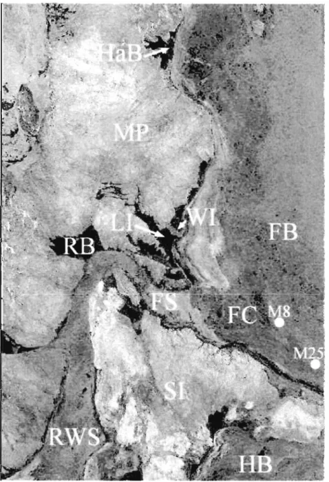
When compared with the satellite image taken during winter (Fig. II.9), it is clear that the path followed by the Lagrangian tracers follow closely the location of western FB's
polynyas at HaB, along MP and in LI. This is a strong indication that the dense waters
found at depth in FC originate from these po1ynyas and that hypothesis f) is therefore
supported by the observations. Thus, the results of our numerical experiment suggest that
the dense water current is the result of brine rejection in HaB's polynya and along MP; this
brine f10ws southwards then southwestwards until the topographie break where it cascades
into FC and can combine with the dense waters produced in LI's polynya. Note that at LI's
polynya, dense waters can sink directly at the bottom of the channel through deep convection because of greater depths. Further work involving the polynyas' dynamics, heat
exchanges with the atmosphere and dense water production will be necessary to examine