Comparing the Size of the Middle Class Using the Alienation Component of Polarization

Cahier de recherche/Working Paper 15-11

Comparing the Size of the Middle Class using the Alienation

Component of Polarization

André-Marie Taptué

Abstract:

This paper shows how to compare the size of the middle class in income distributions

using a polarization index that do not account for identification. We derive a class of

polarization indices where the antagonism function is constant in identification. The

comparison of distributions using an index from this class motivates the introduction of

an alienation dominance surface, which is a function of an alienation threshold. We first

prove that a distribution has a large alienation component in polarization compared to

another if the former always has a larger dominance surface than the latter regardless of

the value of the alienation threshold. Then, we show that the distribution with large

dominance surface is more concentrated in the tails and has a smaller middle class than

the other distribution. We implement statistical inference and test dominance between

pairs of distributions using the asymptotic theory and Intersection Union tests. Our

methodology is illustrated in comparing the declining of the middle class across pairwise

distributions of twenty-two countries from the Luxembourg Income Study data base.

Keywords: Alienation, Identification, Middle class, Polarization

1

Introduction

Studies in polarization traditionally use a framework based on alienation and identification, the basic components of polarization introduced byEsteban and Ray(1994). Alienation measures the degree of hostility between groups using distances between incomes and identification measures the degree of identity within groups using income density or group sizes.

A motivation to studying polarization stems from a risk of uprising and social unrest in a polarized society. It is thought that reducing polarization through actions simultaneously targeting alienation and identification can lessen the risk of social unrest. Moreover, polarization is usually linked to the disap-pearance of the middle class leading to a situation where the poor become poorer and the rich richer. The groups of the poor and the rich can then become antagonistic and involve in social conflict. Another con-sequence of the declining of the middle class is the slowdown of the economic activity since individuals in the middle class are considered as the source of the workforce and those who provide a large part of a country tax revenue. Easterly(2001) associates a large share of income for the middle class to a high economic growth.

Moreover, the frequency of social conflict is high in countries with unequal income distributions and it is low in countries with more equal income distributions where people feel more identified to each other. The emergence of social unrest in a society can then be associated mostly to distances between incomes and the alienation component of polarization than to the extent to which people feel alike. In addition, actions that reduce gaps between incomes can also displace individuals from one income group to another in a manner that increases the overall identification and reduces the risk of conflict between groups. Also, measurements of identification depend on polarization sensitivity, an arbitrary parameter that can induce arbitrariness in polarization ordering and limit robustness and consistency. So, it is advantageous to first controlling for the component of alienation, ignoring the identification component of polarization. This procedure helps avoid arbitrariness induced by the measurement of identification and address the problem of the shrinking middle class using the alienation component of polarization accounting only for discrepancies between incomes.

In this paper we investigate a possibility of abandoning the identification component and relying only on the alienation framework in a polarization index when comparing income distributions. When identification is not taken into account, the matter is no longer polarization, but what remains measures the alienation or the inequality-like component of polarization. The concept of inequality component reflects the fact that the alienation component that is maintained in the index is measured by mean dis-crepancies across incomes. We consider a polarization index developed by Duclos et al. (2004) and assume that identification is constant in the economy such that it does not interact with alienation and is not taken into account in the study of polarization.

This development leads to a restricted form of a polarization index that the comparison in two income distributions introduces an alienation dominance surface that can be used to determine whether a distribution is more concentrated in the tails and has smaller middle class than another for a particular class of polarization indices and ranges of alienation thresholds. For instance, an income distribution in which incomes are far from the median means a large alienation and a hollowing out of its middle class. An alienation dominance surface is defined as the proportion of individuals for whom alienation is greater than an alienation threshold. Alienation attributed to an individual is measured as the absolute relative deviation of his income from the median income, an approach that was used by Foster and Wolfson

(2010/1992). Since we are focusing on individuals for whom distances between their incomes and the median exceed certain limits, those individuals might be on the left of the median or on its right and distances will be negative for those on the left. Measuring alienation in absolute value avoids facing the problem of symmetry.

Whetter incomes in a distribution are farther from their median than incomes in another distribu-tion depends on the alienadistribu-tion threshold that has been fixed. But it is difficult in practice to agree on a non-arbitrary value of that threshold and different conclusions can be reached depending on thresholds. To address this difficulty, we adopt the methodology of stochastic dominance that allows us to determine a range of alienation thresholds, set robust comparisons and establish a partial ordering between two distributions.

Statistical inference is performed to guard against reaching conclusions that may be due to noise in samples. The comparison mentioned above leads to dominance curves that can intersect in the range of alienation thresholds. Also, distances between curves may be too tiny even when one curve always lies above another. One way to take this into account is to test statistically the significance of observed dominance. Thus, the second part of this paper develops statistical inference for stochastic dominance tests using an estimator of the alienation dominance surface. We implement statistical inference with asymptotic theory by deriving the asymptotic sampling distribution of the estimator and testing domi-nance using Intersection Union tests.

We begin inSection 2by first showing the decomposition of some polarization indices in order to isolate the components of alienation and identification. Section 2 also addresses the measurement of alienation and establishes the relation between a polarization index and the alienation dominance surface. This relation characterizes the class of polarization indices compatible with comparison of income distributions in the alienation component of polarization.

The alienation dominance surface is developed explicitly in Section 3 in the particular case of income distributions. This section identifies a distinction between an alienation dominance surface and an inequality measurement on the one hand, and similarities between alienation dominance and bi-polarization dominance on the other hand. Section 3 also establishes the link between alienation

dominance surface and middle class measurements. Section 4 introduces an empirical illustration by comparing income distributions of 22 countries using 2004 data from the Luxembourg Income Study database. Section 5 provides statistical inference by deriving the asymptotic properties of an estimator of the alienation dominance surface and testing statistically the results obtained inSection 4. Finally, Section 6concludes.

2

Methodology

2.1 Decomposition of polarization indices

Our methodology is based on the fact that polarization indices can often be decomposed in a man-ner that isolates the components of alienation and identification. The decomposition gives a possibility of measuring each component alone without accounting for the other component. When one compo-nent is neglected, the antagonism function is written just as a function of the other compocompo-nent. We are examining the situation where the identification component is neglected, in which case the index cap-tures the inequality (alienation) component of polarization. We first examine the decomposition of some polarization indices from the literature on polarization in order to define the measurement of alienation.

The first index we present is that axiomatized byEsteban and Ray(1994) who considered a discrete distribution of income. They measure polarization as the sum of all effective antagonisms in society where the vector of antagonism depends on the levels of alienation and identification for each value of income.

Consider a population of size N where the distribution of income bunches individuals in n groups of incomes y1, y2,··· ,yi,··· ,ynwith sizes ni. The polarization index is proportional to:

ER(η,F) = n

∑

∑

where F is the cumulative distribution function of income and η ∈ (0,1.6] the relative importance of identification and alienation, commonly referred to as a parameter of polarization sensitivity. This polar-ization measure bears resemblance to the Gini coefficient: Equation (1)equals the Gini ifη is set to zero. The fact thatη can exceed zero distinguishes income polarization and inequality. The larger its value, the greater the departure from inequality measurement.

Equation (1)can be rewritten by isolating the two components of polarization:

ER(η,F) = n

∑

∑

The identification felt by group i is ιi = nηi. This measure leads to the same level of identification in

groups with the same sizes. However, identification does not only depend on the number of individuals with similar attributes, but also on the attributes themselves. For instance, the sense of identification must be lower in groups with small income and higher in groups with large income even if these all have the same masses. This view of identification as depending on the levels of attributes yields the following measure of identification:

ιi= nη_iyβ_i (3)

whereβ represents the sensitivity of group cohesion.

Alienation felt by group i towards groups j is|yi− yj|, and the overall alienation felt by group i

towards all the other groups is ai=∑nj=1nj|yi− yj|. Divided by the total size of the population, it is the

sum of alienations between group i and groups j weighted by the population shares of groups j. The total alienation in society is a =∑iniai.

The second index is the index ofDuclos et al.(2004) applicable to a continuous income distribu-tion. It addresses two problems in the index ofEsteban and Ray(1994), that of the discontinuity and the pre-existence of groups in which individuals are clustered. Their index is defined as follows:

DER(η) = ∫∫

f(1+η)(y) f (x)|y − x|dxdy (4)

where f is the income density andη ∈ [0.25,1] is still the polarization sensitivity.

Equation (4)is the continuous form ofEquation (1). The identification generated in a group with income y isι(y) = fη(y). The alienation felt by a group whose income is y towards another group whose income is x is |y − x| such that a∗(y) =∫|y − x|dF(x) is the mean alienation felt by individuals whose income is y towards the rest of the population. A decomposition has been done inDuclos et al.(2004) where the index is rewritten isolating the components of identification and alienation:

DER(η) = ∫

f (y)η ∫

f (y) f (x)|y − x|dxdy. (5)

The average identification is defined by

ι ≡ ∫ f (y)ηdF(y) = ∫

f (y)1+ηdy (6)

and the average alienation in society by

a = ∫ a∗(y)dF(y) = ∫ (∫ |y − x|dF(x) ) dF(y). (7)

Finally, it is proven that

whereρ = cov(a∗(y),_aι ι(y)) is the normalized covariance between alienation and identification.

The alienation component of polarization can also be linked to the middle class and to bi-polarization, which measures the extent to which a population is divided into two separate groups. Foster and Wolf-son (2010/1992) [FW] introduces two polarization curves as well as a new Gini-like index of bi-polarization. The first curve says that bi-polarization is greater when the size of the middle class is smaller, viz., when the distances to the median are larger. The second bi-polarization curve says that bi-polarization is higher when the average distance from the median, on either side of the median, are larger. The index proposed by FW equals twice the area between the Lorenz curve and the tangent to the Lorenz curve at median income.

An income distance between two quantiles at percentiles q−and q+is defined by

S(q−, q+) = Q(q˜ +)− ˜Q(q−) (9)

where ˜Q(q) =_m1F−1(q) is the median (m) normalized income of the person at the qthpercentile. S(q−, q+) is the median-normalized income distance between the two quantiles q−and q+. If [q−, q+_{] overlaps 0.5,}

it can also be thought of as a measure of the size of the middle class. When S is large, there are fewer individuals near the middle, and consequently the middle class is deemed smaller and there is more bi-polarization. FW define a first-order polarization curve as:

S(q) = |S(q,0.5)| (10)

for 0≤ q ≤ 1. For each q, S(q) is the distance that separates median income from the income of the person situated at the q-th percentile. FW also define a second-order polarization curve as

B(p) = 

∫ _0.5

p

S(q)dq (11)

for 0≤ p ≤ 1. B(p) is the area under the S(q) curve between points p and 0.5. The bi-polarization index ofFoster and Wolfson(2010/1992) is then defined as

FW = 2

∫ 1 0

B(p)d p, (12)

which is twice the area beneath the second-order bi-polarization curve B(p).

The measurement of polarization based on the deviation from the median has several extensions.

Wang and Tsui(2000) proposes two extensions that aggregate income distances from the median. The first one uses rank weighting and the corresponding measure is defined by:

W TA =

∫

where w(q) is positive and increasing for q≤ 0.5, and positive and decreasing for q ≥ 0.5. The second one considers a polarization measure defined as a normalized transformation of distances from the median. A class of such indices is given by

W TB =

∫ 1

0 ψ(S(q))dq

(14) whereψ(.) is a continuous function.

2.2 Alienation measurement

At least in some of the indices presented above, alienation for a given income is assessed as the mean distance from some other incomes. The deviation may also be from the mean income, but we choose the median for two main reasons: The first one is the robustness of the median as a statistic compared to the mean income. The median income is not sensitive to the extreme values of a distribution and does not change if these values increase or decrease while the mean will be modified following any change in the extreme values. For the second reason, consider the expression of alienation drawn from the polarization indexEquation (4)ofDuclos et al.(2004) for a continuous distribution of income y.

a∗(y) =

∫

|y − x|dF(x). (15)

We decompose a∗(y) in the sum of the distance when x < y and the distance when x > y:

a∗(y) =

∫

I(x < y)|y − x|dF(x) + ∫

(1− I(x < y))|y − x|dF(x). (16) Thus, alienation in y can exceed a threshold because of the gaps with incomes less than y or because of the gaps with incomes greater than y. The measurement in absolute value allows us to account for the two cases. Notice that alienation in y is the mean of absolute distances between y and all the other incomes. It is known that the median minimizes the expected absolute distance of any variable:

m = arg min

β EX|X − β|. (17)

Consequently, the average absolute deviation from the median is less than or equal to the average absolute deviation from the mean (EX|X − m| ≤ EX|X − µ|) where µ is the mean income. More generally, the

average absolute deviation from the median is always less than or equal to the average absolute deviation from any income quartile.

Therefore, we measure alienation as the relative absolute deviation from the median income. If alienation measured like this is greater than a threshold, then it remains greater when measured as devia-tions from any other fixed income. This method of measuring alienation has already been used byFoster and Wolfson(2010/1992):

a(y) = y

m− 1

Equation (18)defines the degree of alienation attributed to individuals at each level of income. Using this measure in the average alienation expressed inEquation (7)leads to:

a = ∫ (∫  _my − 1dF(x) ) dF(y) (19) = ∫  _my − 1dF(y). (20) 2.3 Comparison principle

Consider two distributions from two distinct populations A and B that we want to compare in the alienation component of polarization in the sense described previously. Let PAbe the polarization index

in population A as defined inDuclos et al.(2004):

PA = ∫∫ p(a, i)dF(a, i) (21) = ∫ _∞ 0 ∫ _∞ 0

p(a, i) f (a, i)dadi (22)

where p(., .) is the antagonism function taking alienation and identification as arguments, F(., .) is the joint cumulative distribution function of alienation and identification and f (., .) the corresponding den-sity. Alienation and identification are two variables defined inR+.

When identification is neglected, the antagonism function does not depend on it. So, p(a, i)∝ p(a) and we can set

PA =

∫ _∞ 0

p(a) f (a)da (23)

where f (a) is the density of alienation. To integrate PA, we proceed first to the substitutionα = −a; then

PA =

∫ 0

−∞p(−α) f (−α)dα (24)

Next, integrating PAby parts yields

PA = p(−α) ∫ _α −∞f (−a)da| α=0 α=−∞+ ∫ ₀ −∞p 1_(−α) (∫ _α −∞f (−a)da ) dα (25) = p(0) ∫ 0 −∞f (−a)da + ∫ 0 −∞p 1_(−α) (∫ _α −∞f (−a)da ) dα (26) = p(0) ∫ _∞ 0 f (a)da + ∫ _∞ 0 p1(α) (∫ _∞ α f (a)da ) dα (27)

where p1is the first-order derivative of the antagonism function with respect to its first argument (alien-ation).

Let za≥ 0 be a value of alienation and let HA(za) =

∫_∞

za fA(a)da denote the alienation dominance surface for population A. Hence, HA(0) = 1 and

PA = p(0) +

∫ _∞ 0

p1(α)HA(α)dα. (28)

The dominance surface is defined analogously for distribution B whereEquation (28)is also applicable:

PB = p(0) +

∫ _∞ 0

p1(α)HB(α)dα. (29)

Let I1denote the class of polarization indices in the form ofEquation (23)where the antagonism function is increasing in alienation and constant in identification:

I1={P in the form ofEquation (23)| p1≥ 0}. (30) We are searching conditions under which PA− PB≥ 0 for any P ∈ I1:

PA− PB=

∫ _∞ 0

p1(α)(HA(α) − HB(α))dα. (31)

Consider P ∈ I1 and suppose that HA(α) − HB(α) ≥ 0 whatever the value of alienation α ≥ 0.

Since p1≥ 0, ∆P = PA−PB≥ 0 for the integral of a positive function in a closed interval is positive. That

is, the condition HA(α) − HB(α) ≥ 0 ∀ α ≥ 0 is a sufficient condition to compare distributions A and B

in the alienation component of polarization when polarization indices are taken in the class I1.

For the necessity condition, suppose that PA− PB≥ 0 for all P ∈ I1 and that on the other side,

HA(α) − HB(α) < 0 for α ∈ [α,α + ε] for a small value of ε > 0. We define an antagonism function by:

p(α,ι) ∝ p(α) =          α if α ≤ α α if α < α ≤ α + ε α + ε if α > α + ε

The function p(α) is increasing in α and ∈ I1_{. The first derivative of that function is p}1_{(α) =} ∂p(α)

∂α = 1 in [α,α + ε] and 0 elsewhere. So,Equation (31)becomes: PA− PB =

∫ _α+ε

α (HA(α) − HB(α))dα. (32)

With the hypothesis that HA(α)−HB(α) < 0, we also have

∫_α+ε

α (HA(α) − HB(α))dα < 0 which implies

that PA−PB< 0 and contradicts the assumption of PA−PB≥ 0. The necessary condition is then verified.

From now on, we denote by zaa threshold of alienation. When HA(za)−HB(za)≥ 0 for all za≥ 0,

we say that the inequality (alienation) component of polarization in distribution A is always greater or equal than that in distribution B. We note B≽ A to express that distribution B stochastically dominates distribution A in the alienation component of polarization.

This relation reports that distribution B is more concentrated around its median and less in its tails than distribution A, or that groups in B are less heterogeneous than groups in A. According to the necessity condition, if there exists a level of alienation zafor which HA(za)− HB(za) < 0, then we argue

that the inequality (alienation) component of polarization in distribution A is not always greater or equal than that in distribution B.

Proposition 2.1 I1dominance: Given two distributions from two distinct populations A and B, B≽ A for all P ∈ I1iff HA(za)− HB(za)≥ 0 for all za≥ 0.

3

Case of income distributions

This section develops an alienation dominance surface for particular cases of income distribu-tions. Income refers to any cardinal variable, such as wealth or wage. We intend to show in this section how the alienation dominance surface is distinct from inequality and how it is linked to a middle class measurement and bi-polarization.

3.1 Alienation dominance surface

Let YA_{= y}A

1, yA2,··· ,yANA and Y

B_{= y}B

1, yB2,··· ,yBNB be two vectors, of sizes NA and NB, of inde-pendent and identically distributed income observations randomly drawn from two populations A and B. The objective is to compare the two distributions in the alienation component of polarization. Alienation can then be measured for each value of income usingEquation (18). For an alienation threshold, say za,

consider the alienation dominance surface

HA(za) = ∫ _∞ za dF(aA(y)) (33) = ∫

I(aA(y)≥ za)dFA(y) (34)

where FA(.) is the cumulative distribution function of income in a population A and I(.) the indicator

function which is equal to 1 if its argument is true and 0 otherwise.

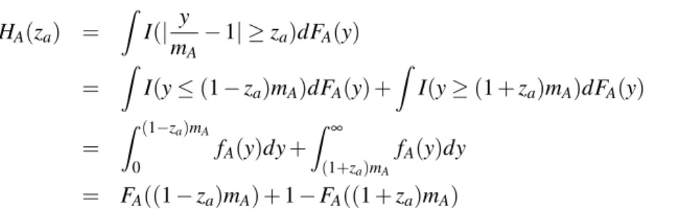
as follows: HA(za) = ∫ I(| y mA− 1| ≥ za )dFA(y) (35) = ∫ I(y≤ (1 − za)mA)dFA(y) + ∫ I(y≥ (1 + za)mA)dFA(y) (36) = ∫ _(1−za)mA 0 fA (y)dy + ∫ _∞ (1+za)mA fA(y)dy (37) = FA((1− za)mA) + 1− FA((1 + za)mA) (38)

where mAis the median of the income distribution in population A.Proposition 2.1 becomes

B≽ A for all P ∈ I1iff FA((1 + za)mA)− FA((1− za)mA)≤ FB((1 + za)mB)− FB((1− za)mB). (39)

Thus, fixing a threshold za induces an interval which is a function of za and the median income, and

within which each value of income must fall. The problem consists then to assess and compare the proportion of individuals for whom incomes are outside this interval [y−_A, y+_A] where y−_A = (1−za)mAand

y+_A = (1 + zA)mAfor a population A. We conceptualize this interval graphically using the income density.

The interval [y−_A, y+_A] and the dominance surface HA(za) are expressed in the space of income as shown

onFigure 1.

Figure 1: Alienation dominance surface for a population A

HA(za) - -Density curve income: y density f(y) y−_A mA y+_A

Increasing a threshold (za) widens the interval [y−, y+] and diminishes H(za), which tends to zero

for large values of thresholds. When the alienation threshold is greater than 1, the lower bound y− = (1− za)m is negative and can be set to zero if income cannot be negative. In the same manner, when za

decreases, the interval [y−, y+] narrows and H(za) increases and equals 1 when za= 0. Remark that H(1)

3.2 Difference with inequality and (bi)polarization

The Pigou-Dalton principle of transfers stipulates that any rank preserving progressive transfer reduces inequality. Similarly, any rank preserving regressive transfer increases inequality. We are testing wheter this principle is valid for the alienation dominance surface H(za). In the income space (Figure1),

individuals are split in three groups of those below the lower bound (y−), those situated in the interval [y−, y+] and those above the upper bound (y+). Any rank preserving transfer within one of these groups will not affect H(za), but will affect inequality. For instance, suppose a rank preserving progressive

(regressive) transfer within one of these three groups, then inequality will decrease (increase), but the proportion of individuals outside the interval [y−, y+] will not change, that is, H(za) remains unchanged.

Suppose an economy with seven individuals with incomes 10$, 30$, 40$, 50$, 70$, 90$ and 100$. The median of this distribution is 50$. Let’s set the alienation thresholds za= 0.5. Then y− = 25,

y+= 75, and H(0.5) = 3/7. Suppose a transfer of 10$ from the second individual to the fifth individual. The new distribution is 10$, 20$, 40$, 50$, 80$, 90$ and 100$. The median has not changed, the two individuals have moved outside the interval [y−, y+_{] and H(0.5) = 5/7 that has increased. Inequality has}

also increased following the regressive transfer between the two individuals. Then suppose a transfer of ten dollars occurs between the sixth and the seventh individuals in any sense. Inequality increases if it is a progressive transfer and decreases if it is a regressive transfer, but the alienation dominance surface does not change.

Thus, though it is qualified as the inequality component of polarization, our measure of alien-ation dominance surface is different from inequality since it sometime fails to respect the Pigou-Dalton principle of transfers as shown above.

Bi-polarization is characterized by increased spread that is the movement away from the median and increased bi-polarity that is the clustering of individuals above and below the median each around their mean incomes. The method of FW measures bi-polarization in the dual space whereas an alienation dominance surface measures it in the primal space. An alienation dominance surface and bi-polarization are affected in the same manner by increased spread, but the impact of increased bi-polarity and that of transfers across the median are ambiguous on an alienation dominance surface.

In the case of increased spread, individuals are moving towards the tails. Bi-polarization as well as the alienation dominance surface H(za) increase regardless of the value of the alienation threshold

za(see Figure 2). The above example with seven persons illustrates the case. The second and the fifth

Figure 2: Increased spread increases bi-polarization and alienation dominance surface regardless of alien-ation threshold H(za) income: y density: f(y) y− m y+

Then consider increased bi-polarity where individuals above and below the median each spread around their mean incomes. Its impact on an alienation dominance surface depends on the size of the alienation threshold and is ambiguous. For small values of za, y− and y+ are close to the median, the

mean of incomes below the median (µL) may be lower than y−, and the mean of those above the median

(µU) may be higher than y+. This is the situation of case 1 inFigure 3where increased bi-polarity can

increase the alienation dominance surface. As za increases, the interval [y−, y+] enlarges, µL may be

higher than y−, and µU may be lower than y+. The case 2 inFigure 3describes this situation in which

increased bi-polarity decreases the alienation dominance surface. However, another situation may occur where nothing can be said about the dominance surface. Take the situation ofFigure 4where µL< y−

and µU< y+ as zamoves. In increased bi-polarity, the increased spread on the left side of the median

increases the alienation dominance surface while the decreased spread on its right induces the opposite effect. The overall effect on the alienation dominance surface is undetermined. An ambiguity is also obtained when µL> y−and µU> y+as zachanges.

Figure 3: Increased bi-polarity can increase (case 1) or decrease (case 2) the alienation dominance surface µL µU y f(y) y− _{m y}+ Case 1 µL< y−and µU> y+ y− y+ y f(y) µL _m µU Case 2 µL> y−and µU< y+

Case 1: individuals are moving outside [y−, y+] and the alienation dominance surface increases.

Case 2: individuals are moving inside [y−, y+] and the alienation dominance surface decreases.

Figure 4: Increased bi-polarity can have an ambiguous effect on the alienation dominance surface

µL µU y

f(y)

y− _m y+

µL< y− and µU< y+

On the left side of the median some individuals are moving outside [y−, y+] while on its right, some

individuals are moving inside. The impact on the alienation dominance surface is undetermined.

Likewise, transfers that displace individuals from one side of the median to another can change the median and can increase or decrease the alienation dominance surface. When the median increases, y− and y+ also increase, the interval [y−, y+] widens and the alienation dominance surface decreases. But when the median decreases, y− and y+ also decrease, the interval [y−, y+] narrows in and the alienation dominance surface increases.

median-normalized distances between the median and incomes of population percentiles:

S(p) = 1 m|F

−1_{(p)− m| (40)}

for 0≤ p ≤ 1. In the primal space, the alienation dominance surface defines a first order dominance curve in alienation with the sum of the proportion of individuals whose incomes are lower than 1− za

times the median and the proportion of those whose incomes are greater than 1 + zatimes the median

across alienation thresholds za:

H(za) = F((1− za)m) + 1− F((1 + za)m) (41)

for za≥ 0. A comparison between the two curves is possible only for values of alienation thresholds less

than or equal to 1 since S(za) is not defined for za> 1. A higher value of S means that there are fewer

incomes near the median. This remark is true for a higher value of H. So, H can be considered as a measure of bi-polarization like S.

3.3 Link with middle class measurements

The alienation dominance surface for a given alienation threshold also relates to the size of the middle class. The most influential measures of the middle class have relied on the position of two income cutoffs around the median and have defined the middle class as the share of the population with income within these cutoffs. The middle class is hence defined as the share of the population with incomes between 75% and 125% of the median income byThurow(1984);Blackburn and Bloom(1985) broaden that middle income range to 60% to 225% of the median income; inLeckie(1988), the middle class is defined on the basis of an income range of 85% to 115% of the median wage. The resulting middle class index, denoted by M, is then the share of the population found within these cutoff points. This index is related to the alienation dominance surface upon the definition of the alienation threshold:

M(za) = 1− H(za) (42)

= F((1 + za)m)− F((1 − za)m). (43)

Graphically, the two measures move in opposite directions (Figure 5). Thus, actions which decrease

H(za) simultaneously increase the middle class (M(za)). Likewise, actions which increase H(za)

Figure 5: Curves of the alienation dominance surface and the size of the middle class as a function of alienation thresholds 0 0.5 1 1.5 2 0 0.2 0.4 0.6 0.8 1 Alienation threshold: za H(za) M(za)

The two curves cross at the alienation threshold z∗_a defined by (0.5− F((1 − z∗_a)m)) + (F((1 +

z∗_a)m)− 0.5) = 0.5. This value of z∗_a can be determined graphically as inFigure 6using the cumulative distribution function of income.

Figure 6: Finding the value z∗_aof the alienation threshold for which H(z∗_a) = M(z∗_a)

Cumulative distribution function

y F(y) m (1− z∗_a)m (1 + z∗_a)m 0.5 F((1− z∗_a)m) F((1 + z∗_a)m)_| {z } 0.5

4

Application

4.1 Data and statistics

We apply the above methodology to 2004 data of 22 countries from the Luxembourg Income Study (LIS) database (seeTable 1). The LIS database contains harmonized microdata from countries which are exclusively middle and high-income countries. It also contains variables on household income, taxes and transfers, households and individual characteristics, labor market outcomes, and expenditures. We use disposable household income, defined as post tax and post transfer income of the household.

The household income is adjusted through the division by an adult equivalent scale s0.5 where s is the household size. This operation is introduced to provide comparable incomes for individuals living in households of different sizes. We also weighted all household observations by the household weight "hweight normalized" multiplied by the number of people in the household unit. Some (less than 0.5%) incomes are negative in each country. We could have set these values to zero but we did not assuming their impact is not significant on results. Income is also normalized by the mean to eliminate the problem of measurement units.

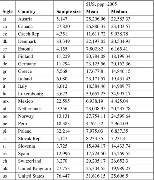
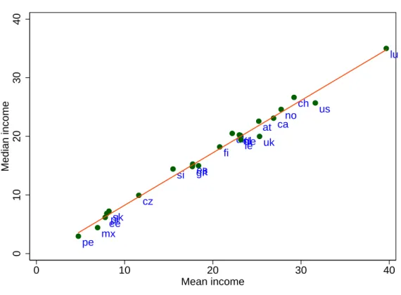
To compute some statistics like the mean and median incomes, the national currencies are con-verted into US $ using the purchasing power parities (PPP) in 2005 from the 2005 International Com-parison Program. Sample sizes for each country are shown in the first column ofTable 1. This table also summarizes the mean and the median of the adjusted household net income of each country set in US $. In addition toTable 1, we plotFigure 7which shows that Luxembourg is far from the others in terms of these two statistics. Its mean income is $39,657.23, the highest among the 22 countries. It is followed by the USA where the mean income is $31,616.15 and then Switzerland with mean of $29,205.55. The lowest mean income is that of Peru ($4,761.52). For the countries like Mexico, Estonia, Poland and Slo-vak Republic, the mean incomes are less than 10,000 dollars, but are greater than that of Peru. The last column ofTable 1presents the median income of the set of the 22 countries. The Luxembourg median income found to be $34,997.17 is still the highest and is far from the rest. It is followed by Switzerland and the USA with the median incomes found to be respectively $26,652 and $25,696,50. The lowest values of the median income are those of Peru ($2,964.09) and Mexico ($4,425.04). These two countries are situated at the bottom South West inFigure 7. In this last figure, countries are all situated close to 45 degree line meaning that their median incomes are almost equal to their mean incomes.

We set the interval of alienation thresholds to be between 0 and 2 for all countries. We first compute the alienation dominance surface for the USA, the country to which we want to compare all others. There is no loss to set the maximum alienation to 2 since few people have income more than three times greater than the median.

Table 1: Sample sizes, mean and median income for 22 countries. Year=2004. $US, ppp=2005

Sigle Country Sample size Mean Median

at Austria 5,147 25,206.96 22,583.33 ca Canada 27,820 26,886.37 23,103.57 cz Czech Rep 4,351 11,611.72 9,938.78 dk Denmark 83,349 22,197.02 20,504.93 ee Estonia 4,155 7,802.82 6,165.41 fi Finland 11,229 20,784.08 18,199.34 de Germany 11,294 23,125.56 20,162.36 gr Greece 5,568 17,677.8 14,846.15 ie Ireland 6,080 23,171.57 19,431.43 it Italy 8,012 18,384.46 14,989.77 lu Luxembourg 3,622 39,657.23 34,997.17 mx Mexico 22,595 6,938.19 4,425.04 nl Netherlands 9,356 23,008.95 20,237.78 no Norway 13,131 27,754.11 24,599.64 pe Peru 18,383 4,761.52 2,964.09 pl Poland 32,214 7,975.03 6,837.35 sk Slovak Rep 5,147 8,233.35 7,231.4 si Slovenia 3,725 15,494.17 14,433.74 es Spain 12,996 17,724.50 15,269.55 ch Switzerland 3,270 29,205.17 26,652.3 uk United Kingdom 27,753 25,304.55 19,989.23 us United States 76,447 31,616.15 25,696.5

Figure 7: Mean and median income (thousands of $ US) of 22 countries at ca cz dk ee fi de gr ie it lu mx nl no pe plsk si es ch uk us 0 10 20 30 40 Median income 0 10 20 30 40 Mean income 4.2 Results

To present results, consider the following question: Among the 22 countries, which ones are better in terms of income concentration around the median, or equivalently which ones are worse in terms of income concentration in the tails of the distribution? We start the application by comparing the 21 other countries to the USA taken as a benchmark. All the countries, except Mexico and Peru, are better than the USA. Whatever the alienation threshold, the alienation dominance surfaces in these countries are lower than that in the USA and their curves always lie under the one of the USA. Thus, these countries stochastically dominate the USA in the alienation component of polarization, but the USA stochastically dominates Mexico and Peru. These results are illustrated both inFigure 8below and in the Figures in the section on statistical tests between the USA and each country.Figure 8shows the difference between the alienation dominance surface of the USA and that of the other countries for each value of the alienation threshold. The difference is negative between the USA and Mexico and between the USA and Peru. This confirms that the alienation dominance surface in these two countries is always greater than that in the USA. Income in the USA is more concentrated around its median (with a large middle class) and less in its tails than income in Mexico and Peru.

Except Mexico and Peru, the curves of the difference between the USA alienation dominance surface and the other countries all lie in the positive area of the plan. Incomes in these countries are more concentrated around their medians and less in their tails than income in the USA regardless of the alienation threshold. InFigure 8the curves of the difference between the USA and Estonia curves and between the USA and UK curves are positive for some alienation thresholds before falling under zero. Before that frontier from which the differences become negative, Estonia and UK stochastically dominate the USA in the alienation component in polarization (see the third panel ofFigure 8).

Then we compare the countries in pairs as shown in Figure 8 andTable 2. Mexico and Peru, whose curves stand out from other countries, are dominated by all the other countries. Above all the curves are located the curve between the USA and Norway, that between the USA and Denmark and the one between the USA and Slovenia. These countries are expected to stochastically dominate all the other countries in a restricted interval of alienation threshold. As zaincreases the difference between the USA

alienation dominance surface and those of the countries of the first group, namely Denmark, Norway and Slovenia exceeds 0.2 for some values of za. For the second group of countries, the difference between

their alienation dominance surfaces and that of the USA exceeds 0.1, but is lower than 0.2. The third group of the countries are those for which the difference between their alienation dominance surfaces and the one of the USA never exceeds 0.1 and the fourth group composed of Mexico and Peru are the countries for which the difference between their alienation dominance surfaces and the one of the USA is always negative.

Figure 8: Curves of the difference between the alienation dominance surface of the USA and those of other countries multiplied by 100

0 0.5 1 1.5 2 0 10 20 0 Dif of alienation dominance surf aces

1st group: the maximal dif is greater than 0.2

dk no si 0 0.5 1 1.5 2 0 5 10 15 20 0

2ndgroup: the maximal dif is > 0.1 and≤ 0.2 at cz fi de lu nl sk pl ch 0 0.5 1 1.5 2 −2 0 2 4 6 8 10 0 Alienation threshold: za Dif of alienation dominance surf aces

3rdgroup: the maximal dif is less than 0.1 ca it gr ee ie uk es 0 0.5 1 1.5 2 −20 −15 −10 −5 0 0 Alienation threshold: za

4thgroup: the difference is negative mx

pe

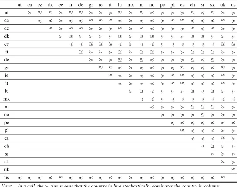
InTable 2, we identify three groups of countries which are similar in terms of income concentration in the tails. The first group is composed of Greece, Ireland, Italy and Estonia where the concentration of income in the tails is almost the same. The second group is composed of some European Northern countries like Norway, Finland and Denmark in addition to Slovenia. Finally the third and last group is composed of the countries of Central Europe like Austria, Czech Republic, Germany and Switzerland.

Table 2: Result of the alienation dominance between 22 countries at ca cz dk ee fi de gr ie it lu mx nl no pe pl es ch si sk uk us at ≽ ≊ ≊ ≽ ≊ ≊ ≽ ≽ ≽ ≊ ≽ ≊ ≼ ≽ ≽ ≽ ≊ ≼ ≊ ≽ ≽ ca ≼ ≼ ≽ ≼ ≼ ≊ ≊ ≊ ≼ ≽ ≼ ≼ ≽ ≊ ≊ ≼ ≼ ≼ ≊ ≽ cz ≊ ≽ ≊ ≊ ≽ ≽ ≽ ≊ ≽ ≊ ≼ ≽ ≽ ≽ ≊ ≼ ≊ ≽ ≽ dk ≽ ≊ ≽ ≽ ≽ ≽ ≊ ≽ ≊ ≊ ≽ ≽ ≽ ≊ ≊ ≽ ≽ ≽ ee ≼ ≼ ≊ ≊ ≊ ≼ ≽ ≼ ≼ ≽ ≼ ≼ ≼ ≼ ≼ ≊ ≊ fi ≊ ≽ ≽ ≽ ≊ ≽ ≊ ≊ ≽ ≽ ≽ ≊ ≊ ≊ ≽ ≽ de ≽ ≽ ≽ ≊ ≽ ≊ ≼ ≽ ≽ ≽ ≊ ≼ ≊ ≽ ≽ gr ≊ ≊ ≼ ≽ ≼ ≼ ≽ ≼ ≊ ≼ ≼ ≼ ≊ ≽ ie ≊ ≼ ≽ ≼ ≼ ≽ ≊ ≊ ≼ ≼ ≼ ≊ ≽ it ≼ ≽ ≼ ≼ ≽ ≊ ≊ ≼ ≼ ≼ ≊ ≽ lu ≽ ≊ ≼ ≽ ≽ ≽ ≊ ≼ ≊ ≽ ≽ mx ≼ ≼ ≽ ≼ ≼ ≼ ≼ ≼ ≼ ≼ nl ≼ ≽ ≽ ≽ ≊ ≊ ≊ ≽ ≽ no ≽ ≽ ≽ ≽ ≊ ≽ ≽ ≽ pe ≼ ≼ ≼ ≼ ≼ ≼ ≼ pl ≊ ≼ ≼ ≼ ≽ ≽ es ≼ ≼ ≼ ≊ ≽ ch ≼ ≊ ≽ ≽ si ≽ ≽ ≽ sk ≽ ≽ uk ≊ us ≼ ≼ ≼ ≼ ≊ ≼ ≼ ≼ ≼ ≼ ≼ ≽ ≼ ≼ ≽ ≼ ≼ ≼ ≼ ≼ ≊

Note: In a cell, the≽ sign means that the country in line stochastically dominates the country in column; the≼ sign means that the country in line is stochastically dominated by the country in column; the≊ sign means that the curve of the country in line is close to the one of the country in column.

5

Estimation and inference

This section is devoted to the development of methods to statistically infer the dominance relation described above. Sometimes, the bulk of observed dominance between two distributions may come from sample noise. For example, suppose Austria is a reference to which we are comparing Poland and Peru.

InFigure 9, we observe that the curve of Austria always lies below those of Poland and Peru, but it is close to that of Poland. Although the curve of Poland is always above the one of Austria, the distance between them is small such that it is difficult to conclude that the two distributions are significantly different in terms of concentration in the tails and that Austria dominates Poland without a statistical test. The two countries might be similar in terms of concentration of income around the median or in the tails of the distribution and the dominance observed in curves could come from noise in samples. The same pattern is observed when the USA is taken as a reference in comparison with Spain and Slovenia. The distance between the USA and Slovenia curves is sufficiently large to indicate the dominance of the USA by Slovenia and that Slovenia is better than the USA. However a conclusion cannot be drawn easily between the USA and Spain. Though the USA curve is always above that of Spain, the distance between the two curves is small and reduce the chance of true dominance of the USA by Spain. It would be more accurate to say that the two distributions are similar in terms of concentration in the queues.

Figure 9: Alienation dominance curves between Peru, Poland and Austria, and between USA, Spain and Slovenia 0 0.5 1 1.5 2 0 0.2 0.4 0.6 0.8 1 Alienation threshold: za Alienation dominance surf ace PERU POLAND AUSTRIA 0 0.5 1 1.5 2 0 0.2 0.4 0.6 0.8 1 Alienation threshold: za USA SPAIN SLOVENIA

So, statistical inference allows to guard against wrong conclusions about dominance induced by sample noise. We propose an estimator of the alienation dominance surface and we verify the conver-gence. Then we test dominance using an Intersection-Union test, an approach introduced by Berger

(1982) and used by Berger and Sinclair (1984) and Berger (1996) that consists of choosing the null hypothesis as a union of simple hypotheses and the alternative hypothesis as an intersection of simple hypotheses.

5.1 Estimator and critical frontiers

Consider a random sample of N independently and identically distributed observations of income

y1,··· ,yN drawn from a distribution with cumulative distribution function F. An estimator of H(za) is

then: ˆ H(za) = ∫ I( ˆa(y)≥ za)d ˆF(y) = N−1 N

∑

∑

where ˆa(y) =|_my_ˆ−1|. The estimator of m is defined by ˆm = in f {y| ˆF(y) ≥₂1} and ˆF(y) = N−1∑N_i=1I(yi≤

y) denotes the empirical distribution function of the sample.

The existence of the population moment of order 1 allows us to apply the law of large numbers toEquation (44)from which we deduce that ˆH(za) is a consistent estimator of H(za). The central limit

theorem allows us to assert that this estimator is root-N consistent and asymptotically normal. Finally, Theorem 5.1that follows defines the asymptotic distribution of the estimator of the alienation dominance surface.

Theorem 5.1 N12( ˆH(z_a)− H(z_a)) is asymptotically normal with mean zero, and the structure of the

variance is given by:

lim

N→∞NVar( ˆH(za)− H(za)) =

1 4 f (m)2[−y

+_{f (y}+_{) + y}−_{f (y}−_)]2

+ (1− F(y+))F(y+) + (1− F(y−))F(y−) (45)

+ 1

f (m)[−y

+_{f (y}+_{) + y}−_{f (y}−_{)](1− F(y}+_{)− F(y}−_)).

Proof: See the Appendix.

The dominance surface H(za) equals 1 when za= 0 and 0 for large values of za. Hence, dominance

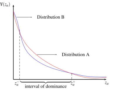
generally exists in an interval of thresholds excluding 0 and large values of alienation. Consider two income distributions from two populations A and B where the interest is about the dominance of A by B. For distribution B to dominate distribution A, there must exist a threshold z−_a from which HA(za) begins

to be greater than HB(za):

z−_a = in f{za|HB(za) < HA(za)}. (46)

From the lower critical frontier z−_a, either HB(za)≤ HA(za) for all za≥ z−a and distribution B stochastically

dominates distribution A everywhere and the maximum alienation threshold can be set to a large value, or else there exists a reversal threshold up to which dominance applies. The upper critical frontier z+_a is the

maximum common alienation threshold up to which distribution B stochastically dominates distribution

A. It is defined by:

z+_a = in f{za> z−a|HA(za) < HB(za)}. (47)

Therefore, z−_a and z+_a are the critical frontiers of the dominance interval as shown inFigure 10.

Figure 10: Critical frontiers and the interval of dominance of distribution A by distribution B

H(za) za z−_a z+_a Distribution B Distribution A | {z } interval of dominance

In this section, we also study the convergence in probability of the estimator of the alienation dominance surface through a Monte Carlo simulation. We first take an alienation threshold za= 0.5. Next

we draw three sets of 1,000 samples from a log-normal distribution of mean zero and standard deviation 1 with sample sizes set respectively to 1,000, 5,000 and 10,000 observations. We draw the density of the estimators obtained from the 1000 simulated samples. InFigure 11, the density curves narrow in as the sample size increases. This behaviour supports the proof that the estimator ˆH(za) is convergent. The

same exercise is conducted for different values of alienation threshold, za= 0.2, 1 and 1.5 and the results

Figure 11: Density curves showing the convergence of ˆH(za) when za= 0.5. For each size N, 1,000

samples are drawn from a log-normal distribution of mean zero and standard deviation 1

0 20 40 60 80 Density .474 .4932 .5124 .5316 .5508 .57

Value of the dominance surface

N=1000 N=5000

N=10000

za= 0.5

Figure 12: Density curves of H(zˆ a) when za = 0.2, 0.5, 1, and 1.5. For sizes N =

1, 000; 5, 000 and 10, 000; 1,000 samples are drawn from a log-normal distribution of mean zero and standard deviation 1 0 20 40 60 80 100 Density 0 .2 .4 .6 .8 1

Values of dominance surfaces

za= 0.2

za= 0.5

za= 1

5.2 Testing dominance

Testing for dominance implies addressing two issues, that of the choice of the null and alternative hypotheses and that of the test statistic. Davidson and Duclos (2000) present three nested hypotheses that could be used either as the null or the alternative hypothesis in dominance tests. The first one is

H0: HA(za)− HB(za) = 0 for all za≤ z+a. The second one is H1: HA(za)− HB(za)≥ 0 for all za≤ z+a

and the third and last one is H2 without any restriction on HA(za)− HB(za). The three hypotheses are

nested in the sense that H0⊂ H1⊂ H2.

McFadden(1989) proposes to test H0 against H1 with the test statistic of the supremum. It is a

form of the Kolmogorov-Smirnov test used to test the identity of two distributions. The main difficulty in the test of McFadden is to trace the asymptotic properties of the test statistic under the null hypothesis. Also, it supposes that the distributions have the same sizes, which is not always the case.

The approach proposed byKaur et al.(1994) [KPS] seems more appropriate. The minimum value of test statistics at different alienation thresholds is used as the test statistic for the null of nondominance against the alternative of dominance. One advantage of this formulation is that if we reject the null hypothesis, all that remains is the alternative of dominance (Davidson and Duclos, 2013). This test is interpreted as the Intersection-Union test (IU) and the probability of rejection of the null when it is true is shown to be asymptotically bounded by the nominal level of a test based on the standard normal distribution (Davidson and Duclos,2000).

So, we propose the following test of H₀aagainst H₁ato test the dominance of A by B: 

 

H₀a: HA(za)≤ HB(za) for some za∈ [z−a, z+a]

H₁a: HA(za) > HB(za) for all za∈ [z−a, z+a].

A procedure to perform this test consists of using a predetermined grid of points corresponding in our case to alienation thresholds (Howes,1993). The only precaution is to be sure to entirely cover the interval of interest. The properties of the IU test using a grid of points are similar to those of the KPS test.

At the tails of the distribution of alienation, the two alienation dominance surfaces are identical. That is HA(0) = HB(0) = 1 and HA(za) = HB(za) = 0 for large values of za. Accordingly, it is impossible

to reject the null of nondominance at the tails of the distributions.

The null hypothesis is a union of simple hypotheses and the alternative hypothesis an intersection of simple hypotheses. In this case, the evidence against the null hypothesis exists when it also exists for every simple null hypotheses. If each simple test is of levelα, then the IU test is also of level α following theorems 1 and 2 ofBerger(1982). Furthermore,Berger and Sinclair(1984) show that not only the IU test is of levelα, but it is exactly of size α.

Consider two distributions drawn from two distinct populations A and B. We suppose that the two distributions are independent. The KPS statistic is defined as the minimum over alienation thresholds of simple test statistics. Consider the following simple test of Hza

0 against H

za

1 for the dominance of A by B

when the alienation threshold is za.

   Hza 0 : HA(za)≤ HB(za) Hza 1 : HA(za) > HB(za)

The test statistic associated to this simple test is

tza=

ˆ

HA(za)− ˆHB(za)

√

Var( ˆHA(za))+Var( ˆHA(za))

Because of the assumption on the independence of the two distributions, the variance of ˆHA(za)−

ˆ

HB(za) is the sum of their variances. Under the null hypothesis, there is no loss to take HA(za) = HB(za),

a condition under which tza tends asymptotically to the standard normal distribution

N

The test statistic of the IU test is defined by: t = min{tza} for zain the grid of thresholds .

Thus, there is a strong evidence against the null hypothesis of the IU test at the nominal levelα if there is a strong evidence against all simple tests. In that case, the test statistic t is greater than the critical value of the standard normal distribution at the levelα.

The evidence against the null hypothesis can also be tested using a p-value. The p-value is de-fined as a measure of the strength of the evidence against the null hypothesis and is determined as the probability of getting a value greater than or equal to the test statistic. Under the null hypothesis, the test statistic above follows the standard normal distribution using the central limit theorem. In consequence, p-value=∫_t∞ϕ(u)du = 1 − Φ(t) where t is the test statistic, ϕ and Φ are respectively the density and the distribution function of the standard normal distribution. Ifα is a given significance level, then reject the null hypothesis if p-value≤ α.

A decision can be taken graphically for each significance level of the test. For instance, consider Figure 13below of the dominance test between two hypothetical distributions A and B, on which we have p-values on the vertical axis and alienation thresholds on the horizontal axis. For this illustrative example and for the traditional significance level of 5%, the null hypothesis is never rejected since p-values are always greater than 0.05 regardless of the threshold. However, the null hypothesis is sometimes rejected when the significance level is set to 10%. In this last case, the null hypothesis cannot be rejected until the threshold equals 0.39. From this threshold, p-values remain less than 10% until the threshold equals 0.51. The critical frontiers can then be fixed respectively to z−_a = 0.39 and z+_a = 0.51, values between

which distribution B stochastically dominates distribution A.

Figure 13: Graphical illustration of a statistical test with p-values at different alienation thresholds

0 0.5 1 1.5 2 2.5 3 0.1 0.2 0.3 0.4 0.5 5· 10−2 0.1 Alienation threshold: za p-v alue

5.3 Application with p-value using LIS data

We now apply this methodology to real data of the 22 countries that we have used for dominance curves in the previous section. We intend to test dominance which has been observed between the 22 countries. We graph the p-values of tests with the null HA(za)≤ HB(za) against the alternative that

HA(za) > HB(za) at various values of alienation thresholds za over a range of 0 to 3. The threshold of

3 is large enough for a dominance interval to encompass potential upper critical frontiers. When the threshold is set to 3, H(3) measures the proportion of individuals whose income is four times greater than the median, a proportion which is very low in most societies.

Graphs are plotted for various pairs of countries. These graphs have an advantage that for different values of significance levels, a conclusion can be drawn on the rejection of the null hypothesis and the critical frontiers can be deduced from the graph.

When the threshold is zero, the p-value always equals 0.5, and no dominance can be expected. So the lower critical frontier must be greater than zero in any case. The critical frontiers also depend on the intervals of the grid such that in cases where the lower critical frontier might be close to zero, it will be set to the first point of the grid.

Statistical tests allow to confirm or not the conclusion drawn from dominance curves. Comparing other countries to the USA, the null hypothesis is the non-dominance of the USA by the other

coun-try (HU SA(za)≤ HCountry(za)) and the alternative is that the USA is dominated by that other country

(HU SA(za) > HCountry(za)).

First consider Mexico and Peru which were shown not to dominate the USA. We are expecting the p-value to be always greater than the significance level of 5% or even 10%. This is exactly what is obtained inFigure 14. The p-values of the test between the USA and Mexico and those between the USA and Peru are never lower than 0.5. This confirms the result obtained with the dominance curves that neither Mexico nor Peru stochastically dominates the USA in the alienation component of polarization. Given that neither the USA and Mexico curves nor the USA and Peru curves were confounded, we run the test the other way around taking the null hypothesis as the alternative and the alternative hypothesis as the null for the three countries. At the significance level of 5%, the test reveals the dominance of Mexico by the USA when the lower critical frontier is z−_a = 0.06 and the upper critical frontier, z+_a, greater than 3. It also shows the dominance of Peru by the USA with the lower critical frontier z−_a = 0.03 and the upper critical frontier greater than 3.

Figure 14: Alienation dominance curves and p-values at different alienation thresholds for the USA and Mexico, and the USA and Peru

0 0.5 1 1.5 2 0 0.2 0.4 0.6 0.8 1 Alienation threshold: za Alienation dominance surf ace /P-v alue P-value MEXICO USA 0 0.5 1 1.5 2 0 0.2 0.4 0.6 0.8 1 Alienation threshold: za P-value PERU USA

Statistical tests confirm the observed dominance in a restricted alienation interval between the USA and Greece and between the USA and Italy. The lower critical frontiers are far from zero in these countries as in Ireland and Spain and shown inFigure 15andTable 3. Despite the relative closeness of the dominance curves of these countries with that of the USA, there exist intervals of alienation within which the USA is stochastically dominated by the two other countries. For Greece, the interval of dominance is [0.24, 0.83] in which the p-value is always lower than 5% and ranges between 0.021 and 0.038. The

dominance interval for Italy is translated on the right compared to that of Greece. Its lower bound is 0.33 and its upper bound 0.96 with p-values of 0.020 for the lower bound and 0.040 for the upper bound. The lower bound of the interval of dominance is 0.42 for Ireland and 0.21 for Spain with p-values set respectively to 0.040 and 0.047. The upper bound is greater than 3 for the two countries.

Figure 15: Alienation dominance curves and p-values at different alienation thresholds for the USA and: Greece, Ireland, Italy and Spain

0 0.5 1 1.5 2 0 0.2 0.4 0.6 0.8 1 Alienation dominance surf ace /P-v alue _USA GREECE P-value 0 0.5 1 1.5 2 0 0.2 0.4 0.6 0.8 1 USA IRELAND P-value 0 0.5 1 1.5 2 0 0.2 0.4 0.6 0.8 1 Alienation threshold: za Alienation dominance surf ace /P-v alue _USA ITALY P-value 0 0.5 1 1.5 2 0 0.2 0.4 0.6 0.8 1 Alienation threshold: za USA SPAIN P-value

Figure 16presents the results of tests where the alienation thresholds are set over an interval of the form [0, z+_a] for various values of z+_a ≤ 2. The null hypothesis is therefore HU SA(za)≤ HCountry(za)

of [0, z+_a]. We notice that the estimator of the alienation dominance surface ˆH(za) in the USA is always

higher than that in other countries, but the distance between the two empirical distribution functions diminishes as z+_a increases and tends to 2. At the significance level of 5%, it is not difficult to see that the null hypothesis of non-dominance is rejected in every threshold range in favour of the alternative of dominance for each z+_a outside a close neighbourhood of zero, because the p-value is always lower than 0.05. The p-values move rapidly from 0.5 for thresholds very close to zero and then stay at zero for every

z+_a.

The USA is then stochastically dominated by the other countries for any alienation threshold in-terval in ]0, 2]. The lower critical frontier is found to be 0.06 for Austria, 0.15 for Canada, 0.09 for the Czech Republic, 0.12 for Luxembourg, 0.06 for Poland, 0.09 for Switzerland, 0.06 for Slovenia and 0.06 for Slovak Republic (SeeTable 3). These lower critical frontiers of the dominance interval are greater than the minimal point of the grid (0.03) and represent a clear estimation of z−_a for the tests between the USA and other countries. The p-values associated to these lower critical bounds ranges from 0.004 in Germany to 0.048 in Poland.

The null hypothesis of non-dominance is rejected until z+_a = 2, leading to an impossibility to define the upper critical frontiers for all these countries. We perform the test once more setting the alienation thresholds over an interval of the form [0, z+_a], but for various z+_a ≤ 3. We verify the results with the above countries for which we first set dominance interval in ]0, 2]. The pattern does not change for z+_a > 2, and

dominance still exists until z+_a = 3. The lower critical frontiers did not change, but still the upper critical frontiers appeared to be greater than 3 for all the countries. Thus, the USA is stochastically dominated for z+_a up to certain point greater than 3. Situations where z+_a are extended to 3 is illustrated inFigure 17where the p-values are always close to zero until z+_a = 3. This confirms the dominance in the entire interval ]0, 3].

Figure 16: Alienation dominance curves and p-values at different alienation thresholds for the USA and: Austria, Canada, Czech Rep, Luxembourg, Poland, Switzerland, Slovenia and Slovak Rep

0 0.5 1 1.5 2 0 0.2 0.4 0.6 0.8 1 Alienation dominance surf ace USA AUSTRIA P-value 0 0.5 1 1.5 2 0 0.2 0.4 0.6 0.8 1 USA CANADA P-value 0 0.5 1 1.5 2 0 0.2 0.4 0.6 0.8 1 Alienation dominance surf ace USA CZECH REPUBLIC P-value 0 0.5 1 1.5 2 0 0.2 0.4 0.6 0.8 1 USA LUXEMBOURG P-value 0 0.5 1 1.5 2 0 0.2 0.4 0.6 0.8 1 Alienation dominance surf ace USA POLAND P-value 0 0.5 1 1.5 2 0 0.2 0.4 0.6 0.8 1 USA SWITZERLAND P-value 0.2 0.4 0.6 0.8 1 dominance surf ace USA SLOVENIA P-value 0.2 0.4 0.6 0.8 1 USA SLOVAK REP P-value

Figure 17: Alienation dominance curves and p-values at different alienation thresholds for the USA and: Denmark, Findland, Germany, Netherlands and Norway

0 0.5 1 1.5 2 2.5 3 0 0.2 0.4 0.6 0.8 1 Alienation dominance surf ace USA DENMARK P-value 0 0.5 1 1.5 2 2.5 3 0 0.2 0.4 0.6 0.8 1 USA FINLAND P-value 0 0.5 1 1.5 2 2.5 3 0 0.2 0.4 0.6 0.8 1 Alienation dominance surf ace USA GERMANY P-value 0 0.5 1 1.5 2 2.5 3 0 0.2 0.4 0.6 0.8 1 USA NETHERLANDS P-value 0 0.5 1 1.5 2 2.5 3 0 0.2 0.4 0.6 0.8 1 Alienation dominance surf ace USA NORWAY P-value

The analysis comparing the USA and other countries shows that dominance always exists when curves are not very close, suggesting dominance when curves are very distant. Consequently, there is no value added to perform the test in pairs between countries especially when the distance between curves is large enough to show clear distinction.

domi-nance according to the alienation domidomi-nance curves as we have done previously. Domidomi-nance tests reveal that dominance can exist even when distance between curves is small. The examples between the USA and Estonia and between the USA and UK are illustrative of these cases. Using the dominance curves, we have concluded that the USA and UK as well as the USA and Estonia cannot be distinguished in terms of alienation dominance and income concentration in the tails or around the median. On the con-trary, statistical tests show dominance between the USA and Estonia on the one hand and between the USA and UK on the other hand. The p-values of the corresponding tests in Figure 18 fall below 0.1 and even below 0.05 for some values of alienation thresholds. The lower and upper critical frontiers between the USA and Estonia are 0.39 with a p-value of 0.046 and 0.60 with a p-value of 0.034. Inside these frontiers, the p-value is always less than 0.05 showing the dominance of the USA by Estonia. The critical frontiers between the USA and UK are 0.18 and 0.9 with corresponding p-values of 0.028 and 0.045. Inside these frontiers, the p-value is lower than 0.05 and is sometimes close to zero, proving that the USA is stochastically dominated by the UK.

Figure 18: Alienation dominance curves and p-values between the USA and Estonia, and the USA and UK at different alienation thresholds

0 0.5 1 1.5 2 0 0.2 0.4 0.6 0.8 1 Alienation threshold: za Alienation dominance surf ace

Alienation dominance curves USA EE UK 0 0.5 1 1.5 2 0 0.2 0.4 0.6 0.8 Alienation threshold: za p-v alue

P-values at different alienation thresholds

US-EE US-UK

We now apply dominance tests only between countries whose dominance curves are close sug-gesting they are similar in terms of income concentration in the tails.

Within the first group composed of Greece, Estonia, Ireland and Italy, we have presumed that these countries are similar based on their dominance curves. With statistical tests, this is exactly the case between Greece and Italy and between Greece and Estonia where the absence of dominance is