HAL Id: tel-02428348
https://tel.archives-ouvertes.fr/tel-02428348
Submitted on 5 Jan 2020HAL is a multi-disciplinary open access archive for the deposit and dissemination of sci-entific research documents, whether they are pub-lished or not. The documents may come from teaching and research institutions in France or abroad, or from public or private research centers.
L’archive ouverte pluridisciplinaire HAL, est destinée au dépôt et à la diffusion de documents scientifiques de niveau recherche, publiés ou non, émanant des établissements d’enseignement et de recherche français ou étrangers, des laboratoires publics ou privés.
massively parallel architectures
Olivier Tissot
To cite this version:
Olivier Tissot. Iterative methods for solving linear systems on massively parallel architectures. Nu-merical Analysis [math.NA]. Sorbonne Université, 2019. English. �tel-02428348�
Sorbonne Université
Inria
Doctoral SchoolSciences Mathématiques de Paris Centre University DepartmentLaboratoire Jacques-Louis Lions
Thesis defended byOlivier Tissot
Defended on 21stJanuary, 2019
In order to become Doctor from Sorbonne Université
Academic Field Applied Mathematics
Iterative methods for solving linear
systems on massively parallel
architectures
Thesis supervised byLaura Grigori
Committee members
Referees Hassane Sadok Professor at Université du Lit-toral Côte d’Opale
Daniel Szyld Professor at Temple University
Examiners Yvon Maday Professor at Sorbonne Univer-sité
Christian Rey Senior Researcher at Safran
Sorbonne Université
Inria
École doctoraleSciences Mathématiques de Paris Centre Unité de rechercheLaboratoire Jacques-Louis Lions
Thèse présentée parOlivier Tissot
Soutenue le 21 janvier 2019
En vue de l’obtention du grade de docteur de Sorbonne Université
Discipline Mathématiques Appliquées
Méthodes itératives de résolution de
systèmes linéaires sur des architectures
parallèles
Thèse dirigée parLaura Grigori
Composition du jury
Rapporteurs Hassane Sadok professeur à l’Université du Lit-toral Côte d’Opale
Daniel Szyld professeur à Temple University
Examinateurs Yvon Maday professeur à Sorbonne Univer-sité
Christian Rey directeur de recherche à Safran
Keywords: linear solvers, parallel computing, Krylov methods, recycling techniques Mots clés : solveurs linéaires, calcul parallèle, méthodes de Krylov, techniques de
This thesis has been prepared at the following research units.
Laboratoire Jacques-Louis Lions 4 place Jussieu
75005 Paris France
T +33 1 44 27 42 98
Web Site http://ljll.math.upmc.fr/
Inria Paris 2 rue Simone Iff 75012 Paris France
T +33 1 80 49 40 00 Web Site http://inria.fr/
xi
Lorsque j’ai un système linéaire à résoudre c’est très simple : j’utilise backslash de Matlab™. Mais je sais qu’il y en a dans la salle pour qui c’est compliqué.
Acknowledgements/Remerciements
Ça y est, je m’attaque aux remerciements. Le reste est fait, je respire depuis un mo-ment. Et, ça n’est pas simple finalement — dire que j’attendais presque cet instant. Déjà, il ne faut oublier personne. Ensuite, il faut satisfaire la curiosité du lecteur, et garder à l’esprit qu’il ne lira très certainement que cette partie. Idéalement, il faut même l’impressionner en faisant de l’esprit, essayer de caler un jeu de mot — une con-trepèterie, c’est un peu trop. Enfin, il faut faire relativement court quand même. Pour l’originalité, c’est compliqué. Apparemment, il y a des règles à respecter123. Et visible-ment plusieurs acteurs sont déjà présents sur le marché du doctorant–peu–inspiré–au-moment–des–remerciements45. Non, ça n’est pas simple finalement...
Je ne dérogerai pas à la règle, et je commencerai par exprimer ma profonde gratitude à Laura. Après ces trois années, je réalise à quel point c’est difficile de mettre des mots sur tout ce que je te dois. Ta confiance et ton soutien tout au long de cette thèse ont été déterminants. Merci de m’avoir proposé ce sujet de thèse. Merci de m’avoir toujours laissé une grande liberté pour aborder les problèmes. Merci pour toutes les opportunités dont j’ai eu la chance de profiter pendant ces trois ans. Merci pour toute l’aide dans la recherche d’un post-doc, et pour avoir eu le soucis de l’après–thèse.
Evidemment, je suis très reconnaissant à Hassane Sadok et Daniel Szyld d’avoir ac-cepté d’être rapporteurs de mon manuscrit de thèse. Merci à Hassane Sadok d’avoir très gentiment accepté d’adapter son emploi du temps afin d’assister à la soutenance. Daniel Szyld, ya que los agradecimientos son en francés y la mayor parte del manuscrito en inglés, he pensado que sería simpático de expresarle en español mis más sinceros agradecimientos por las numerosas correcciones del manuscrito — a pesar de mi (lamentable) nivel de español. Je remercie bien évidemment tout particulièrement Yvon Maday et Christian Rey qui ont accepté de faire partie du jury.
I would like to deeply thank all the members of the NLAFET project, especially Bo Kågström the project leader. I acknowledge HPC2N for providing me the access to Kebnekaise and Abisko.
I deeply thank Jan Papež and Radek Stompor who contributed significantly to the fourth chapter. Thank you Jan to have explained me, more than once, the astrophysics application; thank you, above all, for your help and support. I acknowledge NERSC for providing me the access to Cori and Edison.
Ma mémoire est parfois défaillante mais il y a des choses que je ne peux pas oublier. Je n’oublie pas que Frédéric Bonnans a accepté que je finisse mon contrat un peu plus tôt que prévu pour pouvoir commencer ma thèse dans les meilleures conditions. I do not forget that Jim Demmel hosted me in his group during three months at the 1Nicolas Curien, “Arbres et cartes aléatoires”, HDR. LPMA, Université Pierre et Marie Curie, Paris, 2013.https://www.math.u-psud.fr/~curien/papers/HDR.pdf
2Daniel Pennac, “Merci”, 2004.
3Quentin Verreycken, “Anatomie des remerciements de thèse”, in ParenThèses, 2015, https:// parenthese.hypotheses.org/1127.
4https://www.scribbr.fr/these-doctorat/remerciements-these/
xiii begining of 2016. Je n’oublie pas que Nicole Spillane m’a invité à faire une présentation à DD24. Je n’oublie pas que Iain Duff et Frédéric Nataf ont accepté d’écrire des lettres de recommandation pour moi. Peut-être que pour vous ce n’était pas grand chose, mais pour moi c’était beaucoup : merci à vous.
Pour beaucoup, une thèse c’est–des–hauts–et–des–bas, et je ne fais pas exception. Dans mon cas, ça a aussi été le théâtre de rigolades inoubliables avec Hussam Al-Daas et Sébastien Cayrols. Merci Husssam pour ton sens de l’humour à toute épreuve. Merci Sébastien pour ta gentillesse sans limite. Je ne vous dois pas un merci. Je ne vous dois pas deux mercis. Non, moi je vous dois mille mercis. Votre impact direct et indirect sur mon travail est énorme. En résumé, grâce à vous deux, ma thèse c’est pas la même.
Il y a trois ans, l’équipe Alpines en était à ses balbutiements. Le centre Inria Paris était encore dans les cartons, littéralement. Je remercie sincèrement tous les mem-bres, présents et passés, de l’équipe Alpines qui font qu’elle est toujours une équipe “particulièrement excellente”. Je remercie chaleureusement tous les autochtones du 3A, comprendre 3ème étage du bâtiment A de l’Inria Paris. C’était un vrai plaisir de partager avec vous tous des repas, des cafés, des goûters, des verres, des footings, des baskets, des (baby)foots, et surtout plein de discussions extrêmement enrichissantes; merci pour tout.
Je tiens à remercier la famille Boittin pour son hospitalité. Merci à Martine et Philippe pour les week–ends à Bayeux et tous les très bons restaurants à Paris. Merci à Christine et Dominique, l’antenne Toulouso–Bordelaise, pour le week–end viticole à Bordeaux et le choix toujours cornélien à l’apéro. Merci à Clément pour toutes les anecdotes judiciaires.
Merci à ma famille qui me supporte depuis un certain temps déjà. Mes frères et sœurs Pierre, Laurence, Nathalie et Isabelle qui ont tous essayé de comprendre ce que je faisais. Mes parents m’ont toujours soutenu et, tout en me laissant suivre mon chemin, m’ont donné le goût de la reflexion; merci à vous deux, je me suis souvent dit que j’avais eu bien de la chance de vous avoir. Pendant ces 3 ans, j’ai vu grandir Éloïne, Tristan et Valentin avec un grand bonheur; merci pour tous vos jolis sourires.
Et pour finir, merci à Léa bien sûr. À vrai dire, de simples mots ne peuvent retran-scrire tout ce que je te dois. Je ne suis pas Saint–John Perse alors je me contenterai de te dire merci pour les relectures, les corrections, les encouragements, et le reste surtout.
Et puis merci aussi au pied droit de Benjamin Pavard parce qu’on était mal embar-qué quand même.
Abstract xv
Iterative methods for solving linear systems on massively parallel architectures Abstract
Krylov methods are widely used for solving large sparse linear systems of equations. On dis-tributed architectures, their performance is limited by the communication needed at each it-eration of the algorithm. In this thesis, we first study the use of so-called Enlarged Krylov subspaces for reducing the number of iterations, and therefore the overall communication, of Krylov methods. We consider a reformulation of the Conjugate Gradient (CG) method us-ing these enlarged Krylov subspaces: the Enlarged Conjugate Gradient (ECG) method. This method is first studied from a theoretical point of view. In particular, we show that its conver-gence speed is close to that of the so-called Deflated Conjugate Gradient method. In order to mitigate the effect of the extra arithmetic operations induced by the method, we explain how to dynamically reduce the number of search directions during the iterations. We then present the parallel design of two variants of the ECG method as well as their corresponding dynamic versions. Using a block Jacobi preconditioner, we show that our implementation scales up to several thousands of cores, and it can be significantly faster than the PETSc implementation of the CG method. We then focus on the Cosmic Microwave Background (CMB) analysis. We investigate the usage of so–called recycling strategies in this context. As a result of the multi-plicity of the smallest eigenvalue, these techniques may not improve the convergence in some cases. Hence, we propose a cheap procedure to adapt the initial guess that permits to reduce the overall number of iterations in such situations.
Keywords: linear solvers, parallel computing, Krylov methods, recycling techniques
Méthodes itératives de résolution de systèmes linéaires sur des architectures parallèles Résumé
Les méthodes de Krylov sont largement utilisées pour résoudre des systèmes linéaires creux de grande taille. Sur une architecture distribuée, leur performance est souvent limitée par les com-munications requises à chaque itération de l’algorithme. Dans cette thèse, nous commençons par étudier l’utilisation des sous–espaces dits de Krylov élargis pour réduire le nombre d’ité-rations, et ainsi le nombre de communications, des méthodes de Krylov. Nous nous intéressons à une reformulation de la méthode du Gradient Conjugué (CG) qui utilise ces sous–espaces de Krylov élargis : la méthode du Gradient Conjugué Élargi (ECG). Cette méthode est d’abord étudiée d’un point de vue théorique. En particulier, nous montrons que sa vitesse de conver-gence est proche de celle de la méthode dite du Gradient Conjugué Déflaté. Afin d’atténuer l’effet des opérations arithmétiques supplémentaires requises par la méthode, nous expliquons comment réduire dynamiquement le nombre de directions de recherche pendant les itérations. Nous présentons ensuite le design parallèle des deux variantes de la méthode ECG ainsi que les versions dynamiques qui correspondent. En utilisant un préconditionneur de type bloc Jacobi, nous montrons que notre implémentation est scalable jusqu’à plusieurs milliers de processeurs, et qu’elle peut être significativement plus rapide que l’implémentation de la méthode CG pré-sente dans la librairie PETSc. Nous nous concentrons ensuite sur l’analyse des observations du fond diffus cosmologique. Nous évaluons l’usage des techniques dites de recyclage dans ce contexte. En raison de la multiplicité de la plus petite valeur propre, ces techniques ne per-mettent pas d’améliorer la convergence dans certains cas. Par conséquent, nous proposons une procédure peu coûteuse pour adapter la solution initiale qui permet de réduire le nombre total d’itérations dans ces situations.
Mots clés : solveurs linéaires, calcul parallèle, méthodes de Krylov, techniques de recyclage
Laboratoire Jacques-Louis Lions 4 place Jussieu – 75005 Paris – France
Contents
Acknowledgements/Remerciements . . . xii
Abstract xv Contents xvii List of Figures xxi List of Tables xxiii Introduction (version française) 1 Contexte . . . 1
Résumé et contributions . . . 3
Introduction (English version) 7 Context . . . 7
Summary and contributions . . . 9
1 Preamble 15 1.1 Background in Linear Algebra . . . 16
1.2 Krylov Subspace Methods . . . 18
1.2.1 Derivation of the Conjugate Gradient algorithm . . . 19
1.2.2 Convergence study . . . 21
1.3 Preconditioners . . . 22
1.3.1 Incomplete factorization. . . 23
1.3.2 Domain Decomposition . . . 23
1.3.3 Multigrid . . . 25
1.4 Parallel design of Krylov Methods . . . 26
1.4.1 Mitigating the effect of communication . . . 26
1.4.2 Searching in several directions at once . . . 27 xvii
2 Enlarged Conjugate Gradients 31
2.1 Introduction . . . 32
2.1.1 The Block Conjugate Gradient method . . . 32
2.1.2 A-orthonormalization algorithms . . . 35
2.2 The Enlarged Conjugate Gradient method . . . 36
2.2.1 Enlarged Krylov Subspaces . . . 36
2.2.2 Derivation of the method . . . 37
2.3 Relationship between Orthodir and Orthomin . . . 39
2.4 Convergence study . . . 44
2.5 Dynamic reduction of the search directions . . . 47
2.5.1 Selection of the search directions . . . 47
2.5.2 Choice of the tolerance. . . 53
2.6 Numerical experiments . . . 57
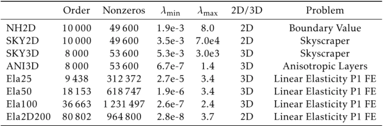
2.6.1 Test cases . . . 57
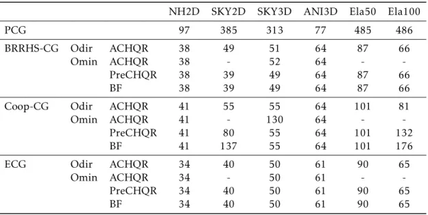
2.6.2 Influence of the parameters and algorithmic variants . . . 59
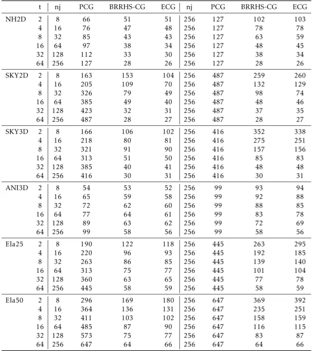
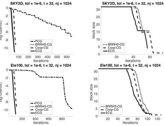
2.6.3 Dynamic reduction of the search directions . . . 61
2.6.4 Numerical comparison with a two–level preconditioner . . . 66
3 Parallel Design 71 3.1 Data distribution . . . 72
3.2 Kernel operations . . . 72
3.3 Cost analysis . . . 74
3.4 Performance results . . . 77
3.4.1 Description of the parallel environment . . . 77
3.4.2 Test cases . . . 79
3.4.3 Results . . . 79
3.5 Fusing global communications . . . 87
3.5.1 Derivation of the algorithm . . . 88
3.5.2 Cost analysis . . . 90
3.5.3 Numerical experiments . . . 91
3.6 Reproducibility of the numerical experiments . . . 94
3.6.1 Implementation details . . . 94
3.6.2 Installation and usage . . . 97
3.6.3 Evaluation and expected result . . . 99
4 Recycling strategies 103 4.1 Motivation — application to CMB data analysis . . . 104
4.1.1 The map–making problem . . . 104
4.1.2 The parametric component separation (PCS) problem . . . 105
4.1.3 The algebraic framework . . . 106
4.2 Ingredients of the methods . . . 107
4.2.1 Eigenvalues approximation using Krylov subspace methods . . . 107
4.2.2 Deflation and two–level preconditioners. . . 110
Contents xix
4.3.1 A priori adaptation of the previous deflation space . . . 114
4.3.2 Solving the system . . . 115
4.3.3 A posteriori update of the deflation space . . . 115
4.3.4 Existing methods . . . 115
4.4 Numerical experiments . . . 117
4.4.1 A simplified case . . . 117
4.4.2 Systems arising from the PCS problem . . . 120
4.4.3 Adaptation of the initial guess for the PCS systems . . . 126
Conclusion 129 Summary . . . 129
Perspectives . . . 130
A Appendices I
A.1 A convergence study of ECG using [89, Theorem 5] . . . I
A.2 Numerical experiments on the BUNDLE test case . . . IV
A.2.1 Impact of the enlarging factor . . . V
A.2.2 Strong scaling study . . . VI
A.3 Numerical experiments on an elasticity problem discretized using PETSc VI
A.3.1 Definition of the problem . . . VI
A.3.2 Numerical results . . . VII
List of Figures
1 Microprocessor trend . . . 8
2 Parallel dot product . . . 9
1.1 Additive Schwarz layout . . . 24
2.1 Splitting of r0 . . . 37
2.2 Block size reduction behavior of D-Odir . . . 64
2.3 Sequential runtimes of ECG D-Odir . . . 66
2.4 Comparison with a 2–level preconditioner on NH2D . . . 68
2.5 Comparison with a 2–level preconditioner on ANI3D. . . 68
2.6 Comparison with a 2–level preconditioner on SKY2D. . . 69
2.7 Comparison with a 2–level preconditioner on Ela50 . . . 69
2.8 Comparison of different types of deflation . . . 70
3.1 Data distribution . . . 72
3.2 Heterogeneity pattern of E and ν for elasticity matrices . . . 78
3.3 Convergence of D-Odir compared to Odir . . . 82
3.4 Strong scaling with threads. . . 85
3.5 Profiling of D-Odir(24) . . . 87
3.6 Numerical comparison between dynamic Orhodir and the fused dynamic Orthodir variant on Flan_1565. . . 91
3.7 Numerical comparison between dynamic Orhodir and the fused dynamic Orthodir variant on Flan_1565. . . 92
4.1 Simplified case experiment with . . . 119
4.2 Simplified case experiment . . . 120
4.3 Convergence results for the first 4 systems of the full sequence with x0= 0121
4.4 Convergence results of the full sequence with continuation . . . 122
4.5 Convergence results for different types of two–level preconditioners . . . 123
4.6 Convergence results for different numbers of deflated vectors . . . 123
4.7 Convergence results for Ritz and harmonic Ritz approximations of the eigenvectors . . . 124
4.8 Eigenvalues of the preconditioned operator for the first system . . . 125
4.9 Convergence of the normalized residual of the third system for different deflated vectors. . . 126
4.10 Convergence of the normalized residual of the second and third systems
when deflating first 5 accurate eigenvectors, and then 6 eigenvectors. . . 127
4.11 Reduced sequence with continuation and adaptation . . . 128
List of Tables
2.1 Matlab test matrices . . . 58
2.2 Numerical parameters . . . 59
2.3 Comparison A-CholQR, Pre-CholQR, and Breakdown-Free . . . 60
2.4 Comparison of BRRHS-CG, ECG, and PCG. . . 62
2.5 Number of iterations of D-Odir . . . 63
2.6 Number of iterations of D-Omin. . . 65
3.1 Complexity of the kernels . . . 74
3.2 Complexity of Orthodir, Orthomin, and CG . . . 76
3.3 Test matrices . . . 79
3.4 Parameter study . . . 81
3.5 Strong scaling study for Flan_1565 . . . 83
3.6 Strong scaling study for Ela_30 . . . 83
3.7 Weak scaling study . . . 86
3.8 Complexity of Orthodir, Fused Orthodir, and CG . . . 91
3.9 Runtime comparison of the fused dynamic Orthodir variant with D-Odir and PETSc’s CG on Kebnekaise . . . 92
3.10 Runtime comparison of the fused dynamic Orthodir variant with D-Odir and PETSc’s CG on Cori . . . 94
4.1 Possible choices of the parameters Vs, M1, M2, M3, Vein Algorithm 18 . 113 A.1 The BUNDLE test case. . . V
A.2 Parameter study for the BUNDLE test case . . . V
A.3 Strong scaling results for BUNDLE. . . VI
A.4 Iteration count and runtimes obtained for an elasticity problem with 81 million of unknown . . . VIII
Introduction (version française)
Sommaire du présent chapitre
Contexte 1
Résumé et contributions 3
Contexte
De nos jours, quasiment tous les ordinateurs, de votre ordinateur portable personnel jusqu’au plus moderne des supercalculateurs en passant par les smartphones, reposent sur le même paradigme : ajouter de plus en plus de processeurs pour calculer de plus en plus vite. Ce paradigme est relativement nouveau : aux alentours de 2005, la fré-quence des processeurs a commencé à stagner autour de 3GHz afin de limiter leur consommation d’énergie (Figure1). En conséquence, le développement de logiciels sur ces architectures parallèle requiert une attention particulière. En effet, sur ces machines parallèles, il est plus coûteux de déplacer des données que de calculer une opération à virgule flottante [42].
Un énorme effort est actuellement déployé afin de développer la première machine exascale, c’est-à-dire capable de calculer 1018opérations à virgule flottante par seconde. Par exemple, en 2015 Barack Obama a signé un décret présidentiel pour créer une “National Strategic Computing Initiative” qui doit découler sur une accélération du développement d’un système exascale. La Chine est censée se doter d’un ordinateur exascale pendant le 13ème Plan Quinquennal (2016–2020). De son côté, la Commission européenne a adopté en 2012 sa stratégie pour le Calcul Haute Performance (HPC en anglais), dont l’un des buts est le développement d’une machine exascale dans les 10 ans. Toutes ces instances ont reconnu qu’il y a un besoin urgent de nouveaux logiciels, et algorithmes, qui seraient efficaces sur ces machines.
Au cœur de cet effort, NLAFET — Algèbre Linéaire Numérique Parallèle pour Sys-tèmes Exascale, est un projet Horizon 2020 FET-HPC financé par l’Union européenne. Son but est de minimiser le fossé entre les capacités maximales théoriques des ma-chines et les performances réalisées en pratiques par les applications HPC qui reposent sur des logiciels d’algèbre linéaire. En pratique, l’objectif est de produire et rendre ac-cessible une libraire, qui serait utilisable comme une boîte noire, pour les parties qui
prennent le plus de temps lors de l’exécution des applications HPC, comme la solution d’un système linéaire. En fait, de la mécanique des fluides numérique [66] jusqu’aux simulations en Astrophysique [113] en passant par l’analyse de données [78], ou l’ima-gerie du cerveau [75], beaucoup d’applications requièrent de calculer la solution d’un système linéaire (éventuellement creux).
Les méthodes pour résoudre les systèmes linéaires sont généralement séparées en deux catégories : les méthodes directes [47] et les méthodes itératives [101]. Les mé-thodes directes sont basées sur la factorisation de la matrice associée au système consi-déré : en général sous la forme d’un produit de matrices triangulaires (LU ), et ensuite la solution est trouvée par substitutions. Ces méthodes calculent la solution de n’im-porte quel système linéaire non singulier en un nombre fini d’opérations, en supposant que l’on néglige les erreurs d’arrondi. En revanche, la quantité de mémoire requise est prohibitive lorsque le système linéaire est très grand. De l’autre côté, les méthodes ité-ratives n’ont besoin de stocker que quelques vecteurs de la taille du système linéaire — même la matrice du système n’a pas besoin d’être stockée explicitement. Néanmoins, la convergence de la méthode est plus sujette aux erreurs d’arrondi, et peut même échouer à trouver une solution acceptable. Afin de prévenir un tel comportement, généralement on ne résout pas le système original Ax = b, mais plutôt le système dit préconditionné M−1Ax = M−1b, où la matrice M−1est proche de la matrice A−1.
En pratique, une itération classique d’une méthode itérative requiert les opérations suivantes :
• la somme de deux vecteurs,
• le produit d’une matrice (creuse) fois un vecteur, • et le produit scalaire de deux vecteurs.
Lorsque le problème devient très grand, il n’est pas possible de stocker un vecteur en entier au sein d’un processeur. Généralement, le vecteur est donc divisé parmi les pro-cesseurs, et chacun d’eux n’en stocke qu’une partie. De la même manière, la matrice ne peut pas être stockée sur un seul processeur. Si l’on suppose que la matrice est creuse, alors un choix simple est de la distribuer par paquets de lignes. Avec ces hypothèses la somme de deux vecteurs est une opération BLAS1 [43] sans communication entre les processeurs. Le produit matrice–vecteur est une opération BLAS2 avec des communica-tions entre les processeurs voisins. Le produit scalaire est une opération BLAS1 suivie d’une communication globale entre tous les processeurs (Figure2).
Du coup, le ratio des communications par rapport aux opérations en virgule flot-tante est élévé, ce qui engendre une mauvaise efficacité sur des machines massivement parallèles. Ceci est particulièrement bien illustré par le benchmark HPCG [44] : en juin 2018, les meilleures machines atteignent environ 1.5% de leur pic de performance lorsqu’elles résolvent un système linéaire creux avec une méthode itérative6!
Résumé et contributions 3
Résumé et contributions
Comme expliqué précédemment, cette thèse fait partie d’un effort global pour amélio-rer la convergence des méthodes itératives afin de :
• diminuer le ratio communication–calcul,
• augmenter le nombre d’opérations en virgule flottante pour tirer parti des nou-velles architectures des micro–processeurs,
• fournir un solveur qui peut être utilisé comme une boîte noire par l’utilisateur final.
Pour atteindre ce but, nous étudions en détail la méthode dite du Gradient Conjugué Élargi (ECG), initialement proposée dans [58]. Ensuite, nous nous intéressons à un pro-blème lié à l’analyse des observations du fond diffus cosmologique (CMB) où plusieurs systèmes linéaires proches les uns des autres doivent être résolus successivement. Dans ce contexte, nous évaluons les bénéfices potentiels ainsi que les limitations des tech-niques dites de recyclage. Il y a quatre chapitres dans le manuscrit.
Dans le Chapitre 1, nous rappelons la méthode du Gradient Conjugué ainsi que d’autres méthodes directement dérivées de celle-ci et particulièrement adaptées au cal-cul parallèle. Plus précisément, nous commençons par rappeler quelques bases d’al-gèbre linéaire. Ensuite, nous rappelons la définition des méthodes dites de Krylov pour résoudre des systèmes linéaires en se concentrant sur le cas où la matrice est symé-trique définie positive. Cela nous mène naturellement à rappeler la définition de la méthode du Gradient Conjugué, ainsi que sa vitesse de convergence. Finalement, nous rappelons quelques méthodes directement dérivées du Gradient Conjugué et qui sont plus adaptées aux architectures parallèles.
Dans le Chapitre2, la méthode du Gradient Conjugué Élargi est étudiée d’un point de vue théorique. Premièrement, nous présentons une dérivation simplifiée de la mé-thode en remarquant qu’elle peut être vue comme un cas particulier des mémé-thodes de Krylov par blocs. Cette analogie nous permet de présenter deux variantes de la mé-thode du Gradient Conjugué : Orthodir et Orthomin. Nous fournissons une explication rigoureuse du manque de robustesse d’Orthomin comparé à Orthodir qui a été observée numériquement. Nous donnons une preuve de la vitesse de convergence de la méthode du Gradient Conjugué Élargi — basée sur une extension de la preuve de [24, Theo-rem 3.2] — qui améliore le précédent résultat existant présenté dans [58]. Cela montre que l’élargissement des sous–espaces de Krylov agit comme un deuxième niveau pour le préconditionneur, qui atténue l’effet des petites valeurs propres sur la convergence de la méthode. Afin d’accroître l’efficacité de la méthode, nous expliquons comment réduire dynamiquement les directions de recherches. En effet, nous montrons qu’en mesurant le rang d’une petite matrice, il est possible de réduire la taille du bloc pen-dant les itérations. Une étude théorique nous donne un critère algébrique pour détecter les directions de recherches qui ont un impact significatif sur la convergence. À partir de cette étude, nous dérivons un choix pratique qui n’induit aucun surcoût et qui véri-fie le critère théorique dans tous nos cas tests. Ce choix ne dépend pas de la méthode
et peut donc être appliqué dans le contexte de la méthode du Gradient Conjugué par blocs en général. Ceci nous permet de comparer différentes méthodes directement dé-rivées de celle-ci, dont la méthode du Gradient Conjugué Élargi. Nous observons que la méthode du Gradient Conjugué Élargi est particulièrement bien adaptée à la réduction des directions de recherche. Elle donne les meilleurs résultats en termes d’efficacité — la taille de l’espace de recherche final est significativement réduite — et robustesse — les erreurs d’arrondi n’ont pas d’impact significatif sur la convergence — dans la grande majorité des cas test numériques que nous avons réalisés.
Dans le Chapitre 3, nous présentons la version parallèle de la méthode du Gra-dient Conjugué Élargi. Nous considèrons à la fois Orthodir et Orthomin, ainsi que les versions dynamiques de ces deux variantes où les directions de recherche sont réduites dynamiquement. La distribution des données et l’analyse du coût de ce design sont pré-sentées en détail. Ensuite, nous présentons des expériences numériques pour évaluer l’efficacité parallèle de ce design ainsi que de la méthode du Gradient Conjugué Élargi sur des machines parallèles. En pratique, nous observons qu’élargir les sous-espaces de Krylov peut entraîner une réduction remarquable du nombre d’itérations. En effet, dans les expériences numériques la méthode est utilisée avec un préconditionneur de type bloc Jacobi, et agit comme un second niveau qui, en quelque sorte, déflate les va-leurs propres les plus petites ; ce qui est en accord avec la théorie présentée dans le Chapitre2. Cela conduit à un gain significatif en termes de temps de calcul comparé à la méthode du Gradient Conjugué classique. À titre d’exemple, pour un problème d’élasticité linéaire en 3D avec des coefficients hétérogènes de taille 4,5 millions (et 165 millions de coefficients non nuls), nous observons que la méthode ECG est jusqu’à 5, 7 fois plus rapide que l’implémentation de la méthode du Gradient Conjugué pré-sente dans PETSc [8], les deux utilisant un preconditionneur de type bloc Jacobi. Ce cas test est connu pour être difficile parce que les preconditionneurs classiques à un niveau ne sont généralement pas très efficaces [36]. Puisque la méthode ECG accroit le nombre d’opérations en virgule flottante tout en réduisant les communications, nous montrons que cette méthode est particulièrement bien adaptée aux architectures mo-dernes et futures qui possèdent un parallélisme massif. Pour le problème d’élasticité précédent, nous montrons que la méthode passe à l’échelle jusqu’à 16, 384 processus, chacun étant attaché à un cœur physique. Nous souhaitons insister sur le fait que notre objectif n’est pas de concevoir un solveur spécifique pour les équations aux dérivées partielles (EDP) elliptiques. Pour ces cas tests, il est très probable qu’il existe des sol-veurs qui sont plus efficaces que la méthode ECG avec un préconditionneur de type bloc Jacobi. Néanmoins, à la différence de ces méthodes, ECG est une méthode algébrique. Elle ne nécessite aucune information sur l’EDP sous-jacente et ne repose sur aucune hypothèse particulière, excepté le fait que la matrice soit symétrique définie positive. Par conséquent elle peut être vue comme un solveur type boîte noire et intégrée très facilement dans un code préexistant. Pour illustrer ceci, nous expliquons en détail com-ment reproduire les expériences numériques. En particulier, nous montrons comcom-ment utiliser notre implémentation et nous fournissons un exemple minimal d’utilisation. Ensuite, nous détaillons la marche à suivre pour reproduire les expériences et
com-Résumé et contributions 5 ment : 1) générer les matrices, 2) télécharger et installer le code, 3) régler les paramètres correctement et soumettre un calcul sur un cluster. Finalement, nous expliquons com-ment améliorer le passage à l’echelle de la méthode en fusionnant les communications globales qui ont lieu lors d’une itération. Nous effectuons des expériences numériques qui montrent une réduction du temps d’exécution par un facteur allant jusqu’à deux lorsqu’on utilise les versions des algorithmes où les communications sont fusionnées.
Dans le Chapitre4, nous étudions les stratégies dites de recyclage afin d’augmen-ter l’efficacité du solveur linéaire dans le contexte de l’analyse des données d’observa-tion du fond diffus cosmologique (CMB). Afin d’effectuer cette analyse, il est nécessaire de résoudre une suite, éventuellement très longue, de systèmes linéaires. A l’intérieur de cette suite, nous supposons que les systèmes changent “peu” les uns par rapport aux autres. Nous examinons les bénéfices possibles qu’il y aurait à utiliser des tech-niques de recyclage. Elles consistent à améliorer dynamiquement le préconditionneur en utilisant de l’information obtenues lors des précédentes résolutions. Plus précisé-ment, l’information recherchée correspond aux vecteurs propres associés aux plus pe-tites valeurs propres de la matrice. Cette information est ensuite incorporée au pré-conditionneur grâce des techniques de type deflation. Nous commencons par rappeler plusieurs méthodes pour calculer les valeurs propres et les vecteurs propres associés d’une matrice à partir d’une base (de Krylov) déjà calculée. Ensuite, nous expliquons comme déflater un sous–espace donné,i.e., supprimer son effet éventuellement néfaste sur la convergence de la méthode de Krylov. Ces deux ingrédient sont la base d’un cadre général pour les méthodes de recyclage que nous présentons ensuite. Des expé-riences numériques sont menées sur des problèmes provenant de l’analyse des données d’observation du fond diffus cosmologique, et l’efficacité de ces méthodes est évaluée d’un point de vue qualitatif. Nous commencons par étudier une situation simplifiée où la matrice sous–jacente est fixée et il y a plusieurs second–membres donnés les uns après les autres. Dans ce cas, les techniques de recyclage nous permettent de réduire le nombre d’itérations significativement. En particulier, lorsque toutes les directions de recherches précédentes sont gardées afin d’approximer les vecteurs propres associés aux plus petites valeurs propres, le nombre total d’itérations est réduit par un facteur jusqu’à 4. Nous étudions ensuite une situtation plus réaliste où à la fois la matrice et les second–membres changent tout au long de la suite. Dans ce cas, ces techniques ne sont pas très efficaces. Les expériences numériques montrent que cela est dû à la mul-tiplicité de la plus petite valeur propre, et que cela est donc inhérent à notre problème. Afin de surmonter cette difficulté, nous proposons une procédure peu coûteuse pour adapter la solution initial avant la résolution. Nous observe alors que le nombre total d’itération est réduit sensiblement. Cette procédure repose sur la structure tensorisée exposée par la matrice sous–jacente.
Pour finir, nous concluons et nous présentons quelques perspectives à ce travail.
Introduction (English version)
Outline of the current chapter
Context 7
Summary and contributions 9
Context
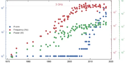
Nowadays almost all the computers, from your personal laptop to the most modern supercomputer including your smartphone, rely on the same paradigm: adding more and more processors to compute faster and faster. This paradigm is relatively new: around 2005 the frequencies of the chips (like a CPU) started to stagnate around 3GHz in order to limit their energy consumption (Figure1). As a consequence a special care has to be taken when designing and implementing software for these parallel architec-tures. Indeed, when addressing such parallel machines it is actually much more costly to move the data than performing floating-point operations [42].
A great effort is currently being put in building the first exascale machine, i.e., a machine that can compute 1018 floating-point operations per second. For instance, in 2015 Barack Obama signed an executive order creating a National Strategic Comput-ing Initiative callComput-ing for the accelerated development of an exascale system. China is supposed to develop an exascale computer during the 13th Five–Year–Plan period (2016–2020). The European Commission adopted in 2012 its High Performance Com-puting (HPC) strategy, one of the goals of which is the development of an exascale machine within 10 years. These instances recognized that there is an urgent need for new software and algorithms that would be effective on such machines.
Being at the heart of this effort, NLAFET — Parallel Numerical Linear Algebra for Extreme Scale Systems, is a Horizon 2020 FET-HPC project funded by the European Union. Its goal is to minimize the gap between the peak capabilities of the hardware and the performance realized by HPC applications relying on linear algebra software. In practice, it aims at delivering a library that would be used as a black–box for the most time–consuming parts of the HPC applications software such as computing the
7https://github.com/karlrupp/microprocessor-trend-data/blob/master/LICENSE.txt
Figure 1 – Microprocessor trend over the last 40 years. Credits: original data col-lected and provided under Creative Commons License7by M. Horowitz, F. Labonte, O. Shacham, K. Olukotun, L. Hammond, C. Batten, and K. Rupp.
solution of a linear system. In fact, from computational fluid dynamics [66], to as-trophysics simulations [113] including data analysis [78], or brain imaging [75], many applications require computing the solution of a (possibly sparse) linear system.
The methods for solving linear systems are usually split into two categories: direct methods [47] and iterative methods [101]. Direct methods rely on the factorization of the original system matrix in a simpler form: usually a product of triangular matrices (LU ), and then the solution is found using backward and forward substitution. They compute the solution of any non singular linear system in a finite number of operations, assuming that round–off errors are neglected. However, their memory requirement is prohibitive when the linear system is very large. On the other hand, iterative methods usually require storing only few vectors of the size of the linear system — even the system matrix does not have to be stored explicitly. However, the convergence of the process is more prone to round–off errors, yielding to delay in the convergence, and even failure to find an acceptable solution. To prevent such undesired behavior, one usually does not solve the original system Ax = b but rather a preconditioned system M−1Ax = M−1b where M−1is close to A−1.
In practice, a typical iteration of an iterative method usually requires the following operations:
• the sum of two vectors,
• the product of a (sparse) matrix times a vector, • and the dot product of two vectors.
When the problem becomes very large it is not possible to store an entire vector in one processor. Usually the vector is split among the processors, and each one of them
Summary and contributions 9 only stores a part of it. Similarly, the matrix cannot be stored in one processor. If we assume that the matrix is sparse, then a simple choice is to distribute the matrix by row panels among the processors. With these assumptions, the sum of two vectors is a BLAS1 [43] operation without any communication. The matrix–vector product is a BLAS2 operation involving communication between neighboring processors. The dot product is a BLAS1 operation followed by a global communication among all the processors (Figure2).
P
1P
2P
3P
4Figure 2 – Schematic workflow of a parallel dot product when the vectors are dis-tributed among 4 processors (P1, P2, P3and P4). The straight lines are representing
com-munication through the network.
Thus the communication–to–computation ratio of iterative methods is high, result-ing in poor efficiency on massively parallel machines. This is well illustrated by the HPCG benchmark [44]: in June 2018, the best machines reach around 1.5% of their peak performance when solving a sparse linear system with an iterative method8!
Summary and contributions
As explained previously, this thesis is part of a global effort for enhancing iterative methods in order to:
• decrease the communication–to–computation ratio,
• increase the arithmetic intensity to take advantage of the new microprocessor architectures,
• provide a solver that can be used as a black–box for the end–user. 8http://icl.utk.edu/hpcg/custom/index.html?lid=155&slid=295
To achieve this goal, we study in thorough details the so–called Enlarged Conjugate Gradient method (ECG) originally proposed in [58]. Then, we study a problem related to the data analysis of the cosmic microwave background (CMB) where several linear systems, that are close to each other, have to be solved successively. In this context, we evaluate the potential benefits and limitations of the so–called recycling techniques. There are four chapters in the manuscript.
In Chapter 1, we recall the Conjugate Gradient method as well as other methods directly derived from it, and specially designed for parallel computing. More precisely, we start by recalling some basics about linear algebra. Then, we recall the definition of the Krylov methods for solving linear systems focusing on the case where the ma-trix is SPD. This naturally leads us to recall the derivation of the Conjugate Gradient algorithm, and the study of its convergence speed. Finally, we recall several methods directly derived from the Conjugate Gradient which are more adapted to parallel ar-chitectures.
In Chapter2, the Enlarged Conjugate Gradient method is studied from a theoret-ical point of view. First, we present a simplified derivation of the method by noticing that it can be seen as a special case of a block Krylov method. This analogy also al-lows us to present two variants of the Enlarged Conjugate Gradient method: Orthodir and Orthomin. We provide a rigorous justification of the lack of robustness of Or-thomin compared to Orthodir that has been observed experimentally. We give a proof of the speed of convergence of the Enlarged Conjugate Gradient method — based on an extension of the proof of [24, Theorem 3.2] — which greatly improves the previous existing result presented in [58]. This shows that enlarging the Krylov subspaces acts as a second level preconditioner that mitigates the effect of the smallest eigenvalues on the convergence of the iterative method. In order to increase the efficiency of the method, we explain how to dynamically reduce the search directions. Indeed, we show that by monitoring the rank of a small matrix, it is possible to reduce the size of the block during the iterations. A theoretical study gives us an algebraic criterion to detect the search directions that do have a significant impact on the convergence. From this study, we derive a practical choice that induces no extra cost and verifies the theoretical criterion in all our test cases. This choice does not depend on the method and therefore can be applied in the context of the Block Conjugate Gradient method. This allows us to compare several methods derived from it, including the Enlarged Conjugate Gradi-ent method. We observe that the Enlarged Conjugate GradiGradi-ent method is particularly adapted to the reduction of the search directions, it leads to the best results in terms of effectiveness — the size of the final search space is significantly decreased — and robustness — the round–off errors do not have a significant impact on the convergence — in most of the numerical tests performed.
In Chapter 3, we present the parallel design of the Enlarged Conjugate Gradient method. We consider both Orthodir and Orthomin variants, as well as dynamic ver-sions of these variants that reduce dynamically the number of search directions. The data distribution and the cost analysis of this design are presented in details. Then, we present numerical experiments to asses the efficiency of this design as well as the
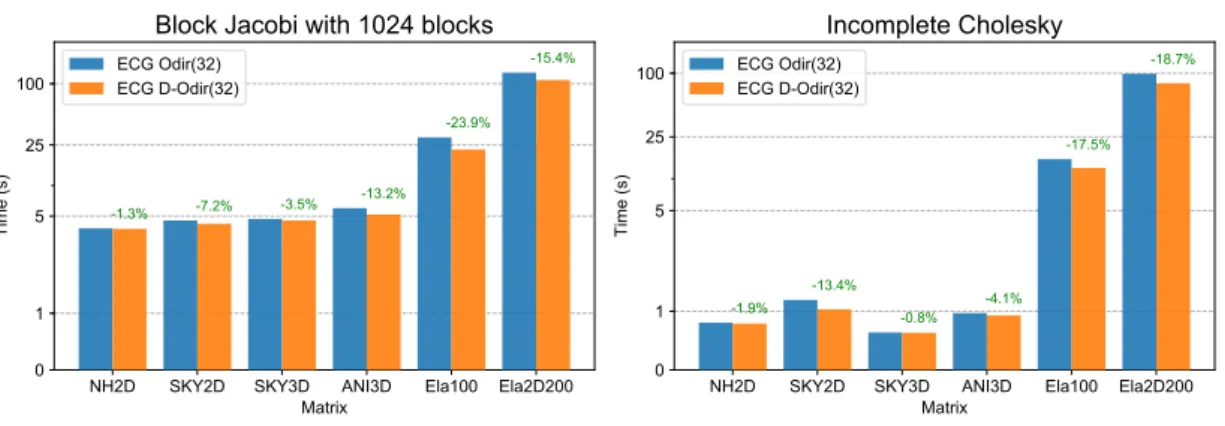
Summary and contributions 11 Enlarged Conjugate Gradient on parallel machines. In practice, we observe that en-larging the Krylov subspaces can drastically reduce the number of iterations. Indeed in the numerical experiments it is used with a block Jacobi preconditioner and acts as a second-level that, in a way, deflates the smallest eigenvalues; this is in accordance with the theory presented in Chapter2. This leads to a significant speed-up over the stan-dard Conjugate Gradient method. For instance for a 3D linear elasticity problem with heterogeneous coefficients with 4.5 millions of unknowns and 165 millions of nonzero entries, we observe that ECG is up to 5.7 times faster than the PETSc [8] implementa-tion of the Conjugate Gradient method, both using a block Jacobi precondiimplementa-tioner. This test case is known to be difficult because the classical one-level preconditioners are not expected to be very effective [36]. As it increases the arithmetic intensity and reduces the communication, we show that it is well suited for modern and future architectures that exhibit massive parallelism. For the previous elasticity problem, we show that the method can scale up to 16, 384 threads, each one being bound to one physical core. We want to point out that our aim is not to design a specific solver for elliptic partial differ-ential equations (PDE). It is very likely that for these test cases, there exists solvers that are more effective than ECG with a block Jacobi preconditioner. Nevertheless, unlike these methods ECG is an algebraic method. It does not require any information from the underlying PDE and does not rely on any assumption, except that the matrix is sym-metric positive definite. Hence it can be seen as a black-box solver and integrated very easily in any existing code. As an illustration, we explain in details how to reproduce the numerical experiments. In particular, we show how to use our implementation and provide a minimal example as an illustration. Then, we detail the workflow for repro-ducing the experiments and how to: 1) generate the matrices, 2) download and install the code, 3) set the proper parameters when submitting the job to a cluster. Finally, we explain how to increase further the scalability of the method by fusing the global communications that occur during one iteration. We perform numerical experiments that show a reduction of the runtime of a factor up to almost two at large scale when using the fused versions of the algorithms.
In Chapter4, we study so–called recycling strategies in order to increase the
effi-ciency of the linear solver in the context of the Cosmic Microwave Background (CMB) analysis. The CMB analysis requires solving a possibly very large sequence of sym-metric positive definite linear systems. Within this sequence, it is assumed that the systems are changing “slowly” from one to the other. Thus we investigate the possible benefits of using recycling techniques which consist in improving the preconditioner dynamically using informations from the previous solve. More precisely, the informa-tion sought is the eigenvectors associated to the smallest eigenvalues of the matrix, and this information is then incorporated in the preconditioner of the next matrix by us-ing deflation. We start by recallus-ing several methods for computus-ing eigenvalues and the associated eigenvectors of a matrix from an already computed (Krylov) basis. Then we explain how to deflate a given subspace,i.e., remove its possibly bad effect on the convergence of the Krylov method. These two ingredients are the basis of the general framework of the recycling methods presented then. Numerical experiments are
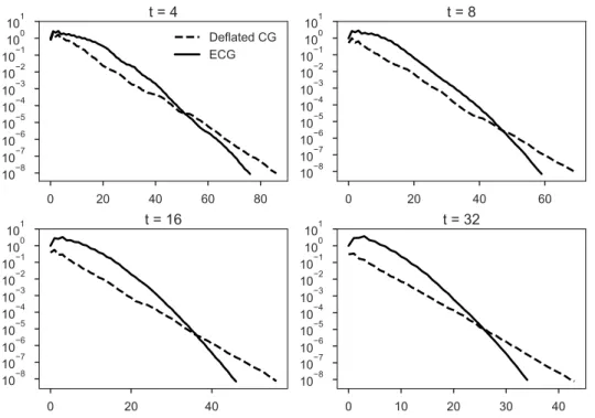
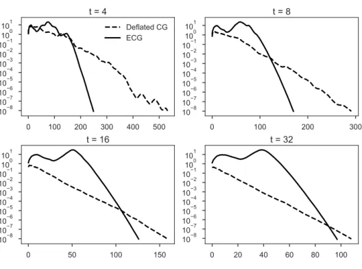
per-formed on problems coming from the CMB analysis, and the efficiency of the methods is assessed from a qualitative point of view. We first study a simplified situation where the underlying matrix is fixed, and there are multiple right-hand sides given one by one. In this case, the recycling techniques allow to reduce the number of iterations significantly. In particular, when all the previous search directions are kept in order to approximate the smoothest eigenvectors the overall number of iterations is reduced by a factor up to 4. We then study a more realistic situation where both the matrix and the right-hand sides are changing through the sequence. In this case, these tech-niques are not very efficient. The numerical experiments show that this is a result of the multiplicity of the smallest eigenvalue, and thus is inherent to our case of interest. In order to overcome this difficulty, we propose a cheap procedure to adapt the initial guess before the solve. It permits to reduce the overall number of iterations noticeably. This procedure relies on the tensorized structure exhibited by the underlying matrix.
Summary and contributions 13 This thesis has lead to the following publications.
Journal papers in revision
L. Grigori and O. Tissot.Scalable Linear Solvers based on Enlarged Krylov subspaces with Dynamic Reduction of Search Directions. Research Report RR-9190. Inria Paris, Laboratoire Jacques-Louis Lions, UPMC, Paris, 2018. Submitted to SIAM SISC.
L. Grigori and O. Tissot. Reducing the communication and computational costs of Enlarged Krylov subspaces Conjugate Gradient. Research Report (old version) RR-9023. Inria Paris, Laboratoire Jacques-Louis Lions, UPMC, Paris, 2017. Submitted to NLAA.
Journal paper in preparation
L. Grigori, J. Papez, R. Stompor, and O. Tissot. Solving sequences of linear systems by recycling deflation subspaces - application to CMB data analysis. In preparation. 2018.
Deliverables of the H2020 NLAFET project
S. Donfack, L. Grigori, and O. Tissot.Deliverable 4.5: Integration. NLAFET deliv-erable. 2018.
M. Abalenkovs et al. Deliverable 5.2: Software integration. NLAFET deliverable. 2018.
S. Donfack, L. Grigori, and O. Tissot. Deliverable 4.4: Performance evaluation. NLAFET deliverable. 2018.
S. Donfack, L. Grigori, and O. Tissot. Deliverable 4.3: Prototype software, phase 2. NLAFET deliverable. 2017.
S. Donfack, L. Grigori, and O. Tissot. Deliverable 4.2: Analysis and algorithm de-sign. NLAFET deliverable. 2017.
1
Preamble
Outline of the current chapter
1.1 Background in Linear Algebra 16
1.2 Krylov Subspace Methods 18
1.2.1 Derivation of the Conjugate Gradient algorithm . . . 19
1.2.2 Convergence study . . . 21
1.3 Preconditioners 22
1.3.1 Incomplete factorization . . . 23
1.3.2 Domain Decomposition . . . 23
1.3.3 Multigrid . . . 25
1.4 Parallel design of Krylov Methods 26
1.4.1 Mitigating the effect of communication . . . 26
1.4.2 Searching in several directions at once . . . 27
Abstract
In this chapter, we recall some background about iterative methods for solving linear systems, focusing on Krylov methods and the Conjugate Gradient method in particular. We start by re-calling basic facts about linear algebra. Then, we explain how to derive the Conjugate Gradient algorithm, a special case of Krylov methods, as well as a well–knwon result about its speed of convergence. In practice, preconditioning is crucial for the method to converge reasonably, and we review some strategies to construct efficient preconditioners. Finally, we present a brief state of the art of the parallel variants of the Conjugate Gradient method.
Résumé
Dans ce chapitre, on rappelle quelques résultats fondamentaux à propos des methodes itéra-tives de résolution de systèmes linéaires, en se concentrant sur les méthodes de Krylov et la méthode du Gradient Conjugué en particulier. On commence par rappeler quelques éléments basiques d’algèbre linéaire. Ensuite, on explique comment dériver l’algorithme du Gradient Conjugué, un cas particulier de méthode de Krylov, ainsi qu’un résultat connu à propos de sa vitesse de convergence. En pratique, le préconditionnement est crucial pour que la méthode
converge raisonnablement et on passe en revue quelques stratégies pour construire des précon-ditionneurs efficaces. Finalement, on présente un bref état de l’art des variantes parallèles de la méthode du Gradient Conjugué.
1.1
Background in Linear Algebra
In this section, we recall some basic results of linear algebra and introduce notations that will be used throughout this thesis. We do not cite explicit references for the results stated in this section. They should be found in any good graduate-level course about linear algebra. In particular, further details can be found in [55,101] for instance1.
In this thesis, we will manipulate mainly two mathematical objects: vectors and matrices. We call v a vector if it is an element of Kn where K = R or K = C, and n > 0 is an integer. For the sake of simplicity, we consider that v is real, i.e., v ∈ Rn. We call A a matrix if it is an element of Km×nwhere K = R or K = C, and m, n > 0 are integers. Similarly, we consider that A is real, i.e., A ∈ Rm×n.
In fact, one should see vectors as columns of real numbers, and matrices as arrays of numbers with m rows and n columns. In spite of the apparent simplicity of these objects, we will see that their study is not that simple. The coefficient at row i and column j of the matrix A is denoted aij. We denote A>the matrix whose coefficient are defined by cij= aji — the rows and columns are switched in the coefficients. Similarly, v>is used to denote a row vector.
We start by the definitions of inner product and norm for vectors. Definition 1.1.1: inner product
Let n ∈ N∗, an inner product on Rnis any mapping denoted h., .i from Rn× Rnto R such that,
1. linearity: ∀v, u1, u2∈ Rn, ∀λ1, λ2∈ R, hλ1u1+ λ2u2, vi = hλ1u1, vi + hλ2u2, vi,
2. symmetry: ∀u, v ∈ Rn, hu, vi = hv, ui,
3. positive definiteness: ∀u ∈ Rn\ {0}, hu, ui > 0 Definition 1.1.2: norm
Let n ∈ N∗, a norm on Rnis any mapping denoted ||.|| from Rnto R+such that, 1. triangle inequality: ∀u, v ∈ Rn, ||u + v|| 6 ||u|| + ||v||,
2. homogeneity: ∀u ∈ Rn, ∀λ ∈ R||λu|| = |λ| ||u||,
3. positive definiteness: ∀v ∈ Rn, ||v|| > 0, and ||v|| = 0 iff v = 0.
1These 2 very popular books cover much more material: [55] focuses on numerical linear algebra, and [101] covers iterative methods for solving linear systems.
1.1. Background in Linear Algebra 17 Intuitively, the norm can be seen as ameasure of a vector — although this does not mean that different vectors should have different norms. An important property that links inner product and norm is the Proposition 1.1.1: given an inner product it is always possible to construct a norm — but the opposite is not true.
Proposition 1.1.1
Given an inner product h., .i, the quantity √
h., .i defines a norm.
We now define the notion of orthogonality which is crucial in all the methods that we will discuss in this thesis.
Definition 1.1.3: orthogonality
Let u, v ∈ Rn, then u, v are said to be orthogonal (denoted u ⊥ v) with respect to h., .i if and only if,
hu, vi = 0. (1.1)
A fundamental theorem, the Riesz representation theorem2, makes the link be-tween the notion of inner product and a special type of matrices. Indeed, one can represent any scalar product using a matrix.
Theorem 1.1.1: Riesz representation
Given an inner product h., .i then there exists a unique matrix A ∈ Rn×n, such that,
∀u, v ∈ Rn, hu, vi = u>Av. (1.2)
Definition 1.1.4: symmetric positive definite matrix A ∈ Rn×nis symmetric positive definite if and only if,
1. symmetry: A>= A,
2. positive definiteness: ∀v ∈ Rn\ {0}, v>Av > 0.
In fact, it is easy to show that any symmetric positive definite (SPD) matrix induces an inner product. Thus, there is an equivalence between SPD matrix and inner product. So given a SPD matrix A, it is straightforward to define an A–norm, denoted ||.||A and an A–orthogonality denoted ⊥A.
2Although its exact statement is much more general, we decided to restrict the presentation to our simplified case where the Hilbert space is simply Rn.
1.2
Krylov Subspace Methods
In this section, we recall the definition of Krylov subspaces methods for solving linear systems. Our presentation is brief and much more details can be found in [101, Chapter 5] and [82, Chapter 2]. We focus on the case where A ∈ Rn×nis SPD, and on the induced method: the Conjugate Gradient (CG) method [68].
Let us recall that we are interested in solving the linear system,
Ax = b, (1.3)
where b ∈ Rn is a given right-hand side x ∈ Rn is the unknown solution. Krylov sub-spaces methods are iterative methods that rely on 2 ingredients: first aprojection pro-cess, second the definition of Krylov subspaces.
First, we briefly explain what is a projection process. Given an initial guess x03, it
searches anapproximate solution xkof the form,
xk∈x0+ Sk, (1.4)
where Skis some k-dimensional subspace of Rn×ncalled thesearch space. The condition (1.4) is also known as thesubspace condition. Of course, this condition is not enough to define uniquely xkand one need to add k constraints on this approximate solution. This is done by enforcing the following condition,
b − Axk⊥ Ck, (1.5)
where Ckis some k-dimensional subspace of Rn×ncalled theconstraints space. The quan-tity b − Axk is also denoted rk and it is called theresidual. The condition (1.5) is also known as the Petrov-Galerkin condition. It is possible to show that if the matrix A is SPD, then Ckcan be chosen equal to Sk ([101, Proposition 5.1] for instance).
It becomes clear that the choice of the subspace Skis crucial as for the efficiency of the resulting method. Here comes into play the second ingredient: the definition of the Krylov subspaces denoted Kk(A, r0). These subspaces are defined such as,
Kk(A, r0) = spannr0, Ar0, . . . , Ak−1r0o. (1.6) One major property of these subspaces is given by Theorem1.2.1[82, Theorem 2.2.3].
Theorem 1.2.1
If r0is of grade d with respect to A, i.e., the degree of the nonzero monic
polyno-mial p of lowest degree such that p(A)v = 0 is d, then r0∈ K1⊂ K2⊂. . . Kd= Kd+j, for all j > 0. Moreover, rd= 0
We want to emphasize on 2 intuitive motivations for searching an approximate so-3It is always possible to choose it equals to 0, if no “good” first guess is known.
1.2. Krylov Subspace Methods 19 lution in these subspaces:
1. the method finds the exact solution x in at most n iterations,
2. the construction of Kk(A, r0) involves a sequence of matrix-vector products which is both simple to implement and relatively cheap.
Remark 1.2.1
In this section and in the rest of this thesis, we focus on the case where A is SPD. In this case, the method of choice is the Conjugate Gradient algorithm. However, when the matrix is not SPD, there exist a lot of Krylov methods such as GMRES [99], BiCGSTAB [118], or QMR [49]. We do not cover these methods in our presentation as we are interested in the case where A is SPD.
1.2.1 Derivation of the Conjugate Gradient algorithm
Following the previous discussion, the iterative process characterized by,
xk∈x0+ Kk(A, r0), (1.7)
rk⊥ Kk(A, r0), (1.8)
is well defined. In particular, we have seen that xnis the exact solution of the original linear system.
From these 2 conditions and the Lanczos algorithm [101, Algorithm 6.15], it is pos-sible to show Lemma1.2.1.
Lemma 1.2.1
Let xk and rk(k ∈ {1, . . . , n}) satisfying the iterative process (1.7)–(1.8), then,
xk= xk−1+ pkαk, (1.9) rk= rk−1−Apkαk, (1.10) where, αk∈ R (1.11) pk∈ Kk(A, r0), (1.12) p>i Apk= 0, i 6 k. (1.13)
Proof. See [101, Section 6.7.1], or [82, Section 2.5.1].
One can easily see that rk∈ Kk+1(A, r0) and rk ⊥ Kk(A, r0). In particular, it is easy to see that rk⊥Api if i 6 k − 1, which is equivalent to p
>
it seems natural to construct pk+1such that,
pk+1= rk−pkβk, (1.14)
where βk is a scalar. In order to determine βk, one has to enforce, p>kApk+1= 0 ⇐⇒ p > kA(rk−pkβk) = 0 (1.15) ⇐⇒ βk= p > kArk p>kApk (1.16)
Similarly, a simple computation allows us to determine αk, p>krk= 0 ⇐⇒ p > krk−1= αk, (1.17) ⇐⇒ αk=p > krk−1 p>kApk. (1.18)
We can notice that p>kApk= ||pk||Aso we can A–normalize the search directions in order to further simplify the expression of αkand βk leading to Algorithm1. This is known as the Conjugate Gradient method [68].
Algorithm 1Conjugate Gradient (CG) 1: r0= b − Ax0
2: p1= r0(r >
0Ar0)−1/2
3: k = 1
4: while ||rk−1||2> εsolver||r0||2and k < kmaxdo
5: αk= pk>rk−1 6: xk= xk−1+ pkαk 7: rk= rk−1−Apkαk 8: βk= p > kArk 9: zk+1= rk−pkβk 10: pk+1= zk+1(z > k+1Azk+1) −1/2 11: k = k + 1 12: end while Remark 1.2.2
The Conjugate Gradient algorithm is sometimes written in a slightly different form where pk is not A–normalized, and βk is expressed in terms of ||rk||2 and ||rk−1||2[101, Algorithm 6.18]. We decided to show this form because it is closer to the algorithm of the Enlarged Conjugate Gradient method.
1.2. Krylov Subspace Methods 21
1.2.2 Convergence study
As the Conjugate Gradient method is an iterative method it is of primary interest to characterize its speed of convergence. First of all, it is possible to prove that the Conju-gate Gradient method finds the approximate solution xkthat minimizes the A–norm of the error over the Krylov subspace Kk(A, r0) (Proposition1.2.2[101, Proposition 5.2]).
Proposition 1.2.1
Let xk (k ∈ {1, . . . , n}) satisfying the iterative process (1.7)–(1.8), then ||x − xk||A= min
y∈x+Kk(A,r0)
||x − y||A (1.19)
Moreover, one can show [82, p. 265] that the approximate residual rkcan expressed as,
rk= qk(A)r0, (1.20)
where qk is a polynomial of degree k, such that qk(0) = 1. We denote Pk1the set of such
polynomials. Moreover, we have rk= A(x − xk) thus,
x − xk= qk(A)(x − x0). (1.21)
Let A = Φ>ΛΦ be the spectral decomposition of A whose eigenvalues are denoted λi (1 6 i 6 n), then we have,
||x − xk||A= ||qk(Λ)Φ(x − x0)||A (1.22) This expression and Proposition1.2.2imply that,
||x − xk||A= min qk∈Pk1 ||qk(Λ)Φ(x − x0)||A (1.23) 6 ||(x − x0)||A min qk∈∈Pk1 ||qk(Λ)||A (1.24) 6 ||(x − x0)||A min qk∈∈Pk1 max 16j6n ||qk(λj)||A (1.25)
Then, it is possible to use Chebyshev polynomials to estimate the min-max quantity [101, Theorem 6.25], min p∈Pk1 max 16i6n |p(λi)| 6 2 √ κ − 1 √ κ + 1 !k , (1.26)
where κ denotes the condition number of the matrix, κ =λmax
λmin.
Finally, a very popular result concerning the convergence of the Conjugate Gradient algorithm follows, ||x − xk||A6 2||x − x0||A √ κ − 1 √ κ + 1 !k (1.27)
Remark 1.2.3
Although very popular, this bounds has several limitations in practice both the-oretical, and practical due to round–off errors (see [82] for a very interesting discussion about these flaws).
1.3
Preconditioners
We have seen that the convergence of the Conjugate Gradient method is related to the condition number κ of the matrix A. To accelerate the convergence of the method, one usually solves a preconditioned system instead of the original one,i.e.,
M−1Ax = M−1b, (1.28)
where M−1A is assumed to have a better condition number than A.
The careful reader may have noticed that this formulation is somehow problematic for the Conjugate Gradient method because M−1A is obviously non–symmetric even if A and M are SPD. However, it is possible to derive a preconditioned version of the Conjugate Gradient method by noticing that M−1A is self–adjoint with respect to the M-inner product,
x>M(M−1Ay) = (M−1Ax)>My = x>Ay. (1.29) Thus, by replacing A by M−1A and> by>M in Algorithm1, it follows the Precondi-tioned Conjugate Gradient algorithm (Algorithm2).
Algorithm 2Preconditioned Conjugate Gradient (PCG) 1: r0= M−1(b − Ax0)
2: p1= r0(r >
0Ar0)−1/2
3: k = 1
4: while ||rk−1||2> εsolver||r0||2and k < kmaxdo
5: αk= p > krk−1 6: xk= xk−1+ pkαk 7: rk= rk−1−Apkαk 8: zk+1= M−1rk 9: βk= p > kAzk+1 10: zk+1= zk+1−pkβk 11: pk+1= zk+1(z > k+1Azk+1) −1/2 12: k = k + 1 13: end while
Of course, the choice of the preconditioner M has a huge impact on the performance of the Krylov method: 1) computing M−1v should be cheap and 2) M−1 has to be as
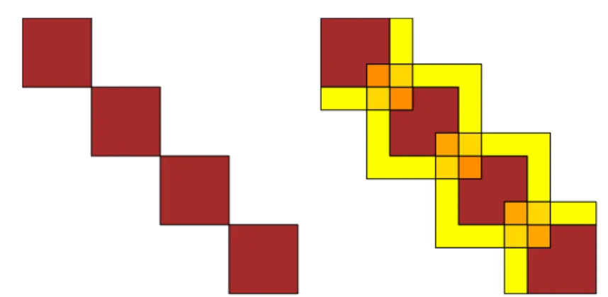
![Figure 2.1 – Illustration of the ordering of A into 8 subdomains obtained with METIS [ 76 ] and several admissible splittings of r 0 into 3 vectors.](https://thumb-eu.123doks.com/thumbv2/123doknet/2305363.25301/62.892.113.726.150.457/figure-illustration-ordering-subdomains-obtained-admissible-splittings-vectors.webp)