O
pen
A
rchive
T
OULOUSE
A
rchive
O
uverte (
OATAO
)
OATAO is an open access repository that collects the work of Toulouse researchers and
makes it freely available over the web where possible.
This is an author-deposited version published in :
http://oatao.univ-toulouse.fr/
Eprints ID : 10092
To cite this version : Rigo-Mariani, Rémy and Sareni, Bruno and
Roboam, Xavier A fast optimization strategy for power dispatching in a
microgrid with storage. (2013) In: IECON 2013 - 39th Annual
Conference of the IEEE Industrial Electronics Society, 10 November
2013 - 13 November 2013 (Vienne, Austria).
Any correspondance concerning this service should be sent to the repository
administrator:
[email protected]
A Fast Optimization Strategy for Power Dispatching
in a Microgrid With Storage
Remy Rigo-Mariani*, Bruno Sareni*, Xavier Roboam*
* Université de Toulouse, LAPLACE, UMR CNRS-INPT-UPS, site ENSEEIHT, 2 rue Camichel, 31 071 Toulouse, France − e-mail: {rrigo-ma, sareni, roboam}@laplace.univ-tlse.fr Abstract—This paper proposes a fast strategy for optimal
dispatching of power flows in a microgrid with storage. The investigated approach is based on the use of standard Linear Programming (LP) algorithm in association with a coarse but linear model of the microgrid. The control references resulting from the LP optimization are adapted in order to comply with a finer model which takes nonlinear features (efficiencies) into account. This approach allows simulating long periods of time and estimating the cost effectiveness with regard to various energy price policies. It would lead to a systemic optimization that would integrate the management strategy device sizing.
Keywords—microgrid, storage, optimal dispatching, linear programming, dynamic programming
I. INTRODUCTION
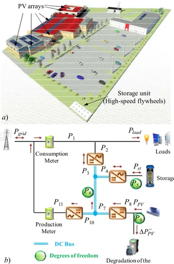
With the growing number of renewable energy sources, major changes have occurred in electrical grid architecture in the past ten years. In the near future, the grid could be described as an aggregation of several microgrids both consumer and producer [1]. For those "prosumers", a classical strategy consists in selling all the highly subsidized production at important prices while all consumed energy is purchased [2]. Smarter operations now become possible with developments of energy storage technologies and evolving price policies [3]. Those operations would aim at reducing the electrical bill taking account of consumption and production forecasts as well as the different fares and possible constraints imposed by the power supplier [4]. The microgrid considered in the paper is composed of a set of industrial buildings and factory with a subscribed power of 156 kW and a PV generator with a peak power of 175 kW (Fig. 1a). A 100 kW/100 kWh storage consisting in the association of ten high-speed flywheels is also introduced and will have to be operated as efficiently as possible. The strategy chosen to manage the overall system is based on a daily off-line optimal scheduling of power flows for the day ahead. Then, in real time, an on-line procedure adapts the same power flows in order to correct errors between forecasts and actual measurements [5]. Several algorithms have been investigated in previous works to perform the off-line optimization for a single day but the high computational times observed did not comply with a sizing procedure that would require many simulations of the microgrids over long periods of time (e.g., weeks, months, year) [6]. The present study focuses on a faster approach consisting in two steps. Firstly, a basic Linear Programming (LP) algorithm solves the cost minimization problem with a coarse linear model of the system as in [7]. Then, a second procedure adapts the obtained solutions to comply with the requirements of a finer nonlinear model. The
paper is organized as follows. The first section describes both coarse and fine models used to represent the system and the various considered hypotheses. Then, the second section presents the fast optimization approach and gives details about adaptation of the control references resulting from the LP optimization. In section III, the results on a test day are presented, by considering particular production and consumption forecasts and according to given energy price policies. Various power dispatching algorithms are compared with regard to their performance and computational time. Finally, a whole year is simulated and the obtained results are discussed with respect to the investment cost of the storage unit.
Fig. 1: Studied microgrid - a) 3D view - b) Power flow model PV arrays Storage unit (High-speed flywheels) a) b) Consumption Meter Production Meter Storage Degradation of the PV production DC Bus Degrees of freedom Loads PV P − ΔPPV P1 P2 P3 P4 P5 P6 P7 P8 P9 P10 P11 grid P Pload st P
II. MODEL OF THE STUDIED MICROGRID
A. Power flow model and degrees of freedom
As illustrated in Fig. 1b, the components are connected
though a common DC bus. Voltages and currents are not considered so far and the study only refers to the optimization of active power flows. In the paper the instantaneous values are denoted as Pi(t) while the profiles over the periods of
simulation are written in vectors Pi. Due to the grid policy,
three constraints have to be fulfilled at each time step t:
• P1(t) ≥ 0: the power flowing through the consumption
meter is strictly mono-directional
• P10(t) ≥ 0: the power flowing through the production
meter is strictly mono-directional
• P6(t) ≥ 0: to avoid illegal use of the storage: flywheels
cannot discharge themselves through the production meter
A particular attention is paid to the grid power Pgrid(t)
which should comply with requirements possibly set by the power supplier: ) ( ) ( ) (t P1t P11t Pgrid = − (1) ) ( ) ( ) ( _max min _ t P t P t
Pgrid < grid < grid (2)
The equations between all power flows are generated using the graph theory and the incidence matrix [8]. As illustrated in Fig. 1b, three degrees of freedom are required to manage the
whole system knowing production and consumption:
• P5(t) = Pst(t): the power flowing from/to the storage unit
(defined as positive for discharge power)
• P6(t): the power flowing from the PV arrays to the
common DC bus
• P9(t) = ΔPPV denotes the possibility to decrease the PV
production (MPPT degradation) in order to fulfill grid constraints, in particular when the power supplier does not allow (or limits) the injection of the PV production into the main grid (P9 is normally set to zero).
B. Efficiencies and fine model
A “fine model” is defined taking account of efficiencies of power converters (typically 98 %) and storage losses. These losses are computed versus the state of charge SOC (in %) and
the power Pst using a function Ploss(SOC) and calculating the
efficiency with a fourth degree polynomial ηFS(Pst) (see (3)).
Both Ploss and ηFS functions are extracted from measurements
provided by the manufacturer (Levisys). Another coefficient
KFS (in kW) is also introduced to estimate the self-discharge of the flywheels when they are not used (see (4)). Once the overall efficiency is computed, the true power PFS associated
with the flywheel is calculated as well as the SOC evolution
using the maximum stored energy EFS (here 100 kWh), the time step Δt (typically 1 hour for the off-line optimization) and
the control reference P5.
(
)
(
)
(
())
()(
())
) ( 0 ) ( ) ( ) ( ) ( ) ( 0 ) ( 5 5 5 5 5 5 ⎩ ⎨ ⎧ + = → > − × + = → < t P /η t P t SOC P t P t P t P η t P t SOC P t P t P FS loss FS FS loss FS (3) 100 ) ( ) ( 0 ) ( 100 ) ( ) ( ) ( 0 ) ( 5 5 ⎪ ⎪ ⎩ ⎪⎪ ⎨ ⎧ × Δ × − = Δ + → = × Δ × − = Δ + → ≠ FS FS FS FS E t K t SOC t t SOC t P E t t P t SOC t t SOC t P (4)Due to the bidirectional characteristics of static converters and especially with flywheel efficiency, the overall system is intrinsically nonlinear and suitable methods have to be used to solve the optimal power dispatching problem.
C. Definition of a coarse linear model
In a second step, a coarse model is developed in order to speed up the solving by using a linear formulation of the problem. Converter efficiencies as well as losses within the storage are neglected. This leads to the following simplifications: ⎪ ⎪ ⎩ ⎪ ⎪ ⎨ ⎧ = = = = ) ( ) ( ) ( ) ( ) ( ) ( ) ( ) ( 11 10 8 7 5 4 3 2 t P t P t P t P t P t P t P t P (5) 100 ) ( ) ( ) ( +Δ = − 5 ×Δ × FS E t t P t SOC t t SOC (6)
III. AFAST OPTIMIZATION APPROACH BASED ON LP A. Standard cost minimization with the fine model
The dispatching aims at minimizing the electrical bill for the day ahead. Prices for purchased and sold energy are assumed to be time dependent with instantaneous values respectively denoted as Cp(t) and Cs(t). References of the power flows associated with the degrees of freedom over the simulated period are computed in a vector Pref=[P5 P6 P9].
Once Pref is determinate, all the other power flows are
computed from the forecasted values for consumption and production. Then P1 and P11 are known to estimate the balance
between purchase and sale. Thus, the cost function is calculated as follows for a 24 hours simulated period:
∑
= − = h 24 0 11 1(). () (). () ) ( t s p t P t C t C t P C Pref (7)In previous works, three algorithms were applied in order to solve the dispatching problem with the fine model finding optimal references Pref* [6]. Firstly, a trust-region-reflective
algorithm (TR) that approximates the objective function with a simpler quadratic function is used [9]. From an initial starting solution, the cost is minimized while fulfilling all nonlinear constraints computed in a vector cnl.
0 ) with )) ( ( min arg ] [ = * ≤ = ref nl ref P * 9 * 6 * 5 * ref P P P P c (P P ref C (8)
The second method uses the clearing algorithm, a niching Genetic Algorithm (GA) which preserves diversity in the
population in order to avoid premature convergence [10]. All constraints related to power flows are included in the cost function with a classical exterior penalty approach. The algorithm returns the best individual in the population from a given number of generations:
⎟ ⎟ ⎠ ⎞ ⎜ ⎜ ⎝ ⎛ + = =
∑
i i C( ) . () min arg ] ref nl P * 9 * 6 * 5 * ref [P P P P c P ref λ (9)where the penalty factor λ is set to a sufficiently high value (typically 106) in order to ensure fulfilment of constraints.
Finally, an original self-adaptive approach based on dynamic programming (DP) [11] has been developed in [6]. It consists in a step by step minimization of the storage SOC levels, sampled on the overall range (i.e. [0%-100%]) with given accuracy ΔSOC [12]. The complexity and performance of this algorithm depend on the SOC sampling that determines the number of studied states.
B. LP applied to a coarse model
In this paragraph, the standard fast LP is considered to solve the problem related to the coarse model developed in section II. Such linear approach aims at decreasing CPU time. Using LP imposes to have a linear cost (expressed with a matrix CL) and linear constraints (expressed though a matrix A
and a vector B) The procedure is then run according to [13]:
(
C .P)
AP B ] P P P [ P L ref ref* P * 9 * 6 * 5 * ref ref ≤ == argmin with . (10)
The upper (ub) and lower (lb) bounds of the decision
variables are expressed using the column vector Jn with n
coefficients equal to 1, where n is the number of simulated time steps, i.e. n = 24 for a whole day with Δt = 1h. In particular, the limits of P5 refer to the maximum charge and discharge powers
of the storage with Pst_min= −100 kW and Pst_max = 100 kW.
[
]
[
]
⎩ ⎨ ⎧ × = × × × = PV PV P P J ub J J J lb n st n n n st P P 0 0 max _ min _ (11)The previous cost function C(Pref) is developed for the
coarse model according to the decision variables P5, P6 and P9
(10). Then, the nonlinear term is removed to obtain the matrix CL (see (11)) used in the LP optimization.
(
)
∑
= ⎟⎟⎠ ⎞ ⎜⎜ ⎝ ⎛ − + + − + − = h 24 0 9 6 5 ) ( . ) ( ) ( . ) ( ) ( . ) ( ) ( ) ( . ) ( ) ( . ) ( ) ( t s load p PV s p s p t C t P t C t P t C t P t C t C t P t C t P C Pref (12)(
)
[
T]
s T p T s T p L T s PV T p load ref ref L C C C C C C P C P P P C − − = × + × − = × with ) ( C (13) The constraint matrix A and vector B are built byconcatenating the matrices Ai and Bi used to express each grid
requirement (14), (15), (16), (17) or storage specified limits (18), (19), (20). In the following equations, the identity and zero matrices n×n are denoted as In and 0n, and the lower
triangular is Tn.
[
]
⎩ ⎨ ⎧ = = ≤ × ∈ ≤ + ⇔ ≥ load 1 n n n 1 1 ref 1 1 P B 0 I I A B P A with and ] h 24 .. 0 [ for ) ( (t) ) ( 0 P5 t P6 P t t P load (14)[
]
⎩ ⎨ ⎧ = = ≤ × ∈ ≤ + ⇔ ≥ PV 2 n n n 2 2 ref 2 11 P B I I 0 A B P A p and with ] h 24 .. 0 [ for ) ( ) ( ) ( 0 P6 t P9 t PPV t t (15)[
]
⎪ ⎪ ⎩ ⎪ ⎪ ⎨ ⎧ − − = = ≤ × − − ≤ + ≥ grid_min PV load 3 n n n 3 3 ref 3 grid_min grid P P P B I 0 I A B P A P P and with ) ( ) ( ) ( ) ( ) ( 9 _min 5 t P t P t P t P t P load PV grid (16)[
]
⎪ ⎪ ⎩ ⎪ ⎪ ⎨ ⎧ + − = − − = ≤ × + − ≤ − − ≤ PV load grid_max 4 n n n 4 4 ref 4 grid_max grid P P P B I 0 I A B P A P P and with ) ( ) ( ) ( ) ( ) ( 9 _max 5 t P t P t P t P t P grid load PV (17)The storage SOC has to lie between 0 % and 100 %. An additional constraint is introduced to force the SOC to return to its initial level, i.e. SOC(24 h) = SOC(0) = 50 %: in fact this equality constraint is indirectly set through the inequality of (20) and by means of the cost optimization which naturally leads to fully exploit (i.e. to discharge) the storage device. Constraints are expressed for t=0..24 h using (6):
[
]
⎪ ⎪ ⎪ ⎩ ⎪ ⎪ ⎪ ⎨ ⎧ × × Δ = = ≤ × ∈ × Δ ≤ ⇔ ≥∑
= = n 5 n n n 5 5 ref 5 J B 0 0 T A B P A SOC ) 0 ( 100 with and with ] h 24 .. 0 [ ) 0 ( 100 ) ( 0 0 5 SOC t E t SOC t E i P FS FS t i i (18)(
)
[
]
(
)
⎪ ⎪ ⎪ ⎩ ⎪ ⎪ ⎪ ⎨ ⎧ × − × Δ = ∈ − = ≤ × − × Δ ≤ − ⇔ ≤∑
= = n 6 n n n 6 6 ref 6 J B 0 0 T A B P A SOC ) 0 ( 100 100 with and ] h 24 .. 0 [ with ) 0 ( 100 100 ) ( 100 0 5 SOC t E t SOC t E i P FS FS t i i (19)[
]
⎪ ⎪ ⎩ ⎪⎪ ⎨ ⎧ = × × = ≤ × ≤ ⇔ ≥∑
= = 0 and 0 0 with 0 ) ( ) 0 ( ) h 24 ( h 24 0 5 7 T n T n T n 7 7 7 X B A J J J B A t t t P SOC SOC (20)C. Correction of the obtained solutions
The dispatching problem defined in the previous subsection can quickly be solved in less than one second using a standard LP algorithm e.g. the Matlab© function linprog with sparse matrices. Some preliminary results show that the obtained solutions obviously do not comply with requirements of the fine microgrid model. Fig. 2 illustrates a case for which the solution Pref* obtained with LP is simulated with fine model
equations. It should be noted that a deep discharge occurs at around 22 p.m. The SOC goes down to −25 % with the fine model while it remains to 0 % and fulfills the constraints with the coarse linear model. Taking account of the flywheel losses also leads to slow down the storage charge and to speed up the storage discharge.
Fig. 2: SOC constraint violation with the fine model
In the same way, the cost function returned by the coarse model is not correct. Therefore, the control references (Pref_LP)
relative to the degrees of freedom obtained with the LP in association with the coarse model should be adapted in order to comply with the fine microgrid model. This can be performed using a step by step correction which aims at minimizing the cost while aligning the SOC computed from the fine model with the one resulting from the LP optimization (denoted as SOCLP). At each time step t, the correction procedure is formulated as follows to find the instantaneous optimal references Pi*(t):
(
)
(
)
(
)
⎪ ⎩ ⎪ ⎨ ⎧ Δ + = Δ + ≤ = = ) ( ) ( and 0 ) ( with ) ( min arg )] ( ) ( ) ( ) ( ) ( * 9 * 6 * 5 * t t SOC t t SOC t P t P C t P t P t P t P LP * ref ref t P ref ref t nl c [ (21) The cost function and the bounds associated with the decisions variables are computed similarly to (7) and (11) at a given time step. The additional constraints are computed in the vector ct nl as follows: ⎥ ⎥ ⎥ ⎥ ⎥ ⎦ ⎤ ⎢ ⎢ ⎢ ⎢ ⎢ ⎣ ⎡ − − − − = ) ( ) ( ) ( ) ( ) ( ) ( min _ max _ 10 1 t P t P t P t P t P t P grid grid grid grid t nl c (22)This local minimization problem is solved using the TR
method with a starting point equal to Pref_LP(t). The
convergence is ensured in all cases in a very short CPU time due to its small dimensionality (only three decision variables have to be determined, the P5 decision variable being directly
coupled with the SOC trajectory). Typically, the CPU time related to this correction procedure is less than one second over a day of simulation. The LP algorithm associated with the
previous correction procedure is denoted as LPC in the
following parts.
IV. TEST RESULTS
A. Comparison of dispatching strategies on a single day In this subsection, we compare performance of four dispatching strategies (i.e. TR, GA, DP and LPC) presented in
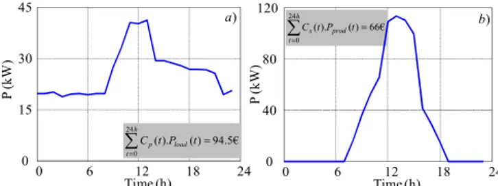
the previous parts, with regard to their accuracy and CPU time. For the considered day, consumption and production forecasts are illustrated in Fig. 3.
Fig. 3: Typical forecasted consumption (a) and production (b)
The consumption profile is extracted from data provided by the microgrid owner while the production estimation is based on solar radiation forecasts computed with a model of PV arrays [14]. Energy prices result from one of the fares proposed by the French main power supplier [15] increased by 30%. Thus, the purchase cost Cp has night and daily values with 0.10 €/kWh from 10 p.m. to 6 a.m. and 0.17 €/kWh otherwise. Cs is set to 0.1 €/kWh which corresponds to the price for such PV plants.
In a situation with no storage device, all the production is
sold (66.0 €) while all loads are supplied through the
consumption meter (94.5 €). In that case, this leads to an overall cost equal to 28.5 € (Fig. 3) for the considered day. It should also be noted that no grid constraints are introduced in the investigated simulations.
Results obtained with TR and GA, are illustrated in Fig. 4. The TR method is successively performed 50 times with different starting points chosen at random within predefined bounds. Each computation takes on average 1 min with 150 iterations at the most. The convergence is only ensured in 24 % of cases and the obtained solutions are not necessary satisfying. Fig. 4a shows the density function associated with the values of the cost function for all computed solutions. The significant deviations between cost function values after convergence indicates that the TR efficiency strongly depends on the initial points. The solutions provided by the GA after 10 000 generations are of equivalent value but the CPU time of 1 hour is far more expensive. However, the GA is more reliable than the TR method with good solutions obtained after only few minutes of computation whatever the initial population. The GA continuously improves the cost function during generations. A cost of 0.7 € has been obtained after 50 000 generations with a corresponding CPU time of 5 hours. As shown in Table I, the DP allows reaching the same cost value with a faster CPU time. In addition, the cost function is further improved when the storage discretization is decreased. The best cost value is obtained with ΔSOC = 1 % but after more than 2 hours. The self-adaptive DP developed in [6] ensures a similar cost while reducing the CPU time down to 10 min.
With the same hypothesis, the LPC reaches an overall cost
of 0.9 € on the considered day. Even if that value does not comply with the best observed, it remains satisfying with regard to the previous results. The best advantage of this strategy is the really fast CPU time: about one second compared to several minutes or more with other algorithms.
Optimal SOC profile obtained with the coarse model
0 6 12 18 24 -25 0 25 50 75 100 SO C (% ) Time (h) Discharge
speeded up Storage limit
SOC profile with Pref*introduced in the finer model
Charge slowed down 0 6 12 18 24 0 15 30 45 Time (h) P ( kW ) a) 0 6 12 18 24 0 40 80 120 Time (h) P ( kW ) b) € 66 ) ( ). ( 24 0 = ∑ = h t prod stP t C € 5 . 94 ) ( ). ( 24 0 = ∑ = h t load pt P t C
Fig. 4: Results obtained with the TR (a) and the GA (b) TABLE I. DPRESULTS
ΔSOC 15 % 10% 5% 1% adaptive
Self-C(Pref*) 4.4 € 3.7 € 1.2 € 0.1€ 0.2
CPU Time 1 min 2 min 9 min 2 h 10 min
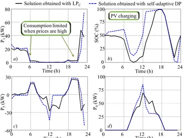
Fig. 5: Results obtained with LPC and self-adaptive DP - a) p1 - b) SOC - c) p5
d) p6
Fig. 5 shows the optimal SOC and the P1 flow profiles
obtained with the self-adaptive DP and LPC. As can be seen in
Fig. 5a, both algorithms try to minimize the cost by lowering as much as possible the power flowing though the consumption meter when the energy prices remain high. The SOC profiles found by both algorithms have similar overall shapes. At the beginning of the day, the flywheel feeds the load in order to reduce the energy consumption issued from the grid. During the day, the PV production is mostly exploited to feed the load and charge the storage. The surplus is sold to generate additional benefit and no production is wasted (P9(t)= 0 ∀t) as the injected power flowing through the
main grid is not limited here. When solar radiation falls down at 8 p.m., the storage is strongly discharged until the price becomes lower at 10 p.m. The storage SOC returns to its initial state of 50 % at the end of the day so as to fulfil the requirements.
As previously underlined, both solutions obtained with the self-adaptive DP and LPC are quite similar with respect to the
overall cost. However, as shown in Fig. 5c-d, the values of decision variables appear to be quite different. This can be explained by the non-uniqueness of the dispatching problem solutions. Indeed, this problem could be considered as an optimal energy balance between purchase, sale, storage charge or discharge. At a given time step and over a period of several hours, different power profiles can led to the same result with regard to the storage energy variations.
B. A whole year simulated with various price policies
Estimating the cost effectiveness of the microgrid from an optimal power dispatching strategy implies to run simulations of longer periods than a single day. Algorithms with “expensive” CPU times cannot be considered in that context. The LPC appears to be the most suitable here leading to the
best compromise with regard to cost and computational time minimizations. It should be reminded that the chosen control is based on an optimal scheduling performed each day for the day ahead. Thus, to simulate a whole year, the LPC procedure
is successively carried out over 365 days. For each run, the storage has to return to the initial SOC value of 50 % at the end of the day.
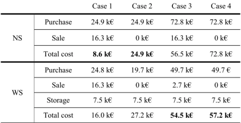
Investment costs of PV arrays are not considered so far as they are already on site. The model only refers to the cost of the storage flywheel estimated at 1500 €/kWh [16]. According to the manufacturer, the flywheel lifetime is ensured on 20 years. Therefore, the storage cost per year is estimated at 7500 € for a 100 kWh unit. Four hypotheses are investigated for the future price policies set by the power supplier that buys or sells energy. Cases 1 and 2 correspond with the fares related to industrial sites [15] with different values between winter and summer. Cases 3 and 4 refer to the actual prices increased by 30 %. Simulations with (i.e. cases 1 and 3) and without (i.e. cases 2 and 4) the payment of the sold energy are also performed.
• Case 1: Cp= 0.05 €/kWh from 10 p.m. to 6 a.m. and
0.08 €/kWh otherwise from November to
March. Cp= 0.02 €/kWh from 10 p.m. to 6 a.m. and 0.03 €/kWh otherwise from April to October. Cs= 0.10 €/kWh.
• Case 2: Cp same as in case 1 and Cs= 0 €/kWh.
• Case 3: Cp= 0.10 €/kWh from 10 p.m. to 6 a.m. and 0.17 €/kWh otherwise. Cs= 0.10 €/kWh. • Case 4: Cp same as in case 1 and Cs= 0 €/kWh.
The obtained results with a storage (WS) controlled by an optimal dispatching are compared with a microgrid with no storage (NS). For the case NS, only purchased and sold energies are considered in the overall cost of the simulated year expressed in k€. The CPU time required to perform 365 runs of 24 h with the LPC in order to estimate the overall energy cost is
about 8 min. 0 2500 5000 7500 10000 0 2 4 6 8 0
Average values after 10 runs Best values after 10 runs
C os tf unc tion (€ ) (b) Number of generations 0.7 €after 50 000 generations 0 0.1 0.2 0.3 Optimal cost (€) De ns ity (a) 0 10 20 30 40 50 60 Cost with no storage Best values at1.1 € 0 6 12 18 24 0 20 40 60 80 Time (h) P1 (k W ) 0 6 12 18 24 0 25 50 75 100 Time (h) SO C ( % )
Solution obtained with LPC Solution obtained with self-adaptive DP
a) b)
PV charging Consumption limited
when prices are high
c) d) 0 6 12 18 24 -60 -30 0 30 Time (h) P5 (k W ) 0 6 12 18 24 0 25 50 75 100 Time (h) P6 (k W )
TABLE II. INVESTMENT COST STUDY WITH VARIOUS PRICE SCENARIOS
Case 1 Case 2 Case 3 Case 4
NS Purchase 24.9 k€ 24.9 k€ 72.8 k€ 72.8 k€ Sale 16.3 k€ 0 k€ 16.3 k€ 0 k€ Total cost 8.6 k€ 24.9 k€ 56.5 k€ 72.8 k€ WS Purchase 24.8 k€ 19.7 k€ 49.7 k€ 49.7 € Sale 16.3 k€ 0 k€ 2.7 k€ 0 k€ Storage 7.5 k€ 7.5 k€ 7.5 k€ 7.5 k€ Total cost 16.0 k€ 27.2 k€ 54.5 k€ 57.2 k€ As seen in Table II, the cost effectiveness strongly depends on the price policy. If prices of the purchased energy remain low (cases 1 and 2) earnings brought by storage do not compensate investment. Shifting consumption when prices are reduced does not improve the overall cost if daily and night fares are close and both at low values. In the same time, if selling the production is highly subsidized (case 1), using a storage is irrelevant because production is always sold to maximize the profit. If buying energy becomes more expensive and prices more variable, managing a storage unit would certainly become interesting with higher benefits brought by the load shifting (cases 3 and 4). The cost effectiveness could even be greater if the fare of the sold power decreases (case 4). This situation could correspond to future price policies that would favor self-consumption as well as optimal use of microgrid components. Note that potential future price policies could offer additional benefits to microgrids ensuring grid services (here, a predictive control of grid trajectory for the day ahead).
V. CONCLUSIONS
The study carried out in this paper aims at proposing a fast procedure in terms of computation time that could be used to investigate cost-effectiveness of a microgrid with storage. In previous works efficient algorithms have been developed to perform the daily scheduling of power flows. However, the main drawbacks of these methods reside in their computational times that become prohibitive if the microgrid has to be simulated over a long period of time. To overcome this problem, a fast optimization approach based on LP has been proposed. This approach consists in two successive steps. Firstly, a coarse linear model of the microgrid is exploited to solve the optimal dispatching with a classical LP algorithm. Secondly, control references optimized with the coarse model are adapted in order to comply with a finer model of the microgrid which takes account of nonlinear features (i.e. efficiencies). The performance of this approach with regard to energy cost minimization and computational time reduction has been shown on a particular test day. Moreover, the fast CPU time resulting from this optimal dispatching method has allowed to simulate the microgrid over a whole year and to investigate its cost effectiveness by considering several scenarios of price policies. The obtained results have shown that the interest of using a storage unit is closely linked to the
economical context. Future studies will be focused on the same issue with other kind of storage technologies such as Li-ion batteries for which cycling effect would have to be included in the cost function. Finally, the fast control algorithm may offer the ability of achieving systemic design of microgrids integrating sizing optimization loop with power dispatching optimization by taking account of system environment and requirements.
ACKNOWLEDGMENT
This study has been carried out in the framework of the SMART ZAE national project supported by ADEME (Agence de l'Environnement et de la Maîtrise de l'Energie). The authors thank the project leader INEO-SCLE-SFE and partners LEVISYS and CIRTEM.
REFERENCES
[1] G. Celli, F. Pilo, G. Pisano, V. Allegranza, R. Cicoria and A. Iaria, “Meshed vs. radial MV distribution network in presence of large amount of DG”, Power Systems Conference and Exposition, IEEE PES, 2004.
[2] A. Campoccia, L. Dusonchet., E. Telaretti, and G. Zizzo, “Feed-in Tariffs for Gridconnected PV Systems: The Situation in the European Community”, IEEE PowerTech, pp.1981-1986, 2007.
[3] S. Yeleti and F. Yong, “Impacts of energy storage on the future power system”, North American Power Symposium (NAPS), pp. 1–7, 2010. [4] C.M. Colson, “A Review of Challenges to Real-Time Power
Management of Microgrids”, IEEE Power & Energy Society General Meeting, pp. 1–8, 2009.
[5] R. Rigo-Mariani, B. Sareni, X. Roboam, S. Astier,., J.G. Steinmetz and E. Cahuet, “Off-line and On-line Power Dispatching Strategies for a Grid Connected Commercial Building with Storage Unit”, 8th IFAC
Power Plant and Power System Control, Toulouse, France, 2012. [6] R. Rigo-Mariani, B. Sareni, X. Roboam and S. Astier, “Comparison of
optimization strategies for power dispatching in smart microgrids with storage”, 12th Workshop on Optimization and Inverse Problems in
Electromagnetism, Ghent, Belgium, 2012.
[7] A. Nottrott, J. Kleissl and B. Washom, “Storage dispatch optimization for grid-connected combined photovoltaic-battery storage systems”, IEEE Power and Energy Society General Meeting, pp 1-7, 2012. [8] S. Bolognani, G. Cavraro, F. Cerruti and A. Costabeber, “A linear
dynamic model for microgrid voltages in presence of distributed generations”, IEEE First International Workshop on Smart Grid Modeling and Simulation (SGMS), pp. 31-36, 2011.
[9] Y. Zhang, “Solving Large-Scale Linear Programs by Interior-Point Methods Under the MATLAB Environment”, Department of Mathematics and Statistics, University of Maryland, Baltimore County, Baltimore, MD, Technical Report TR96-01, 1996.
[10] A. Petrowski, “A clearing procedure as niching method for genetic algorithms”, Proceedings of IEEE evolutionary computation, pp. 798– 803, 1996.
[11] P. Bertsekas, Dynamic programming and optimal control, 2nd Edition, Athena Scientific, 2000.
[12] Y. Riffoneau, S. Bacha, F. Barruel and S. Ploix, “Optimal Power Flow Management for Grid Connected PV Systems With Batteries”, IEEE Transactions on Sustainable Energy, Vol. 2, N°3, pp. 309–319, 2011. [13] S.S. Rao, Engineering Optimization, 4rd ed., Wiley, Hoboken, NJ,
2007.
[14] C. Darras, S. Sailler, C. Thibault, M. Muselli, P. Poggi, J.C Hoguet, S. Melsco, E. Pinton, S. Grehant, F. Gailly, C. Turpin, S. Astier and G. Fontès, “Sizing of photovoltaic system coupled with hydrogen/oxygen storage based on the ORIENTE model”, International Journal of Hydrogen Energy, Vol. 35, N°8, pp. 3322-3332, 2010.
[15] http://france.edf.com [16] http://beaconpower.com