*REG-20021657*
REG-20021657QMUQS
University of Quebec at Montreal P O Box 8889 Succ. Centre-ville . Montreal, QC . CANADA SUBMITTED: ATTN: . 2016-04-28 PHONE: . PRINTED: 2016-04-28 14:18:37 REQUEST NO.: FAX: . REG-20021657
SENT VIA: Manual
E-MAIL: .
8588237 EXTERNAL NO.:
Regular Copy Journal
REG
NOTES:
PAPER COPY TO END-USER
'
REQUESTER INFO: 1764565
DELIVERY: E-mail Post to Web: [email protected]
REPLY: Mail:
Message to Requesting Library
Library Name
Copyright message.Energy-efficient power allocation algorithms for
mobile wireless sensor networks
Fatiha Djemili Tolba*
Computer Science Department, University of Badji Mokhtar, Annaba 23000, Algeria E-mail: [email protected] *Corresponding author
Damien Magoni
LaBRI, University of Bordeaux, Talence 33405, France E-mail: [email protected]Pascal Lorenz
MIPS/GRTC,University of Haute Alsace, Colmar 68008, France E-mail: [email protected]
Wessam Ajib
Computer Science Department, University of Quebec Montréal, Montreal H2X 3Y7, Canada E-mail: [email protected]
Abstract:This paper proposes new distributed algorithms of adaptive transmit power allocation in wireless sensor networks for improving the efficiency of energy management. The proposed algorithms are based on two fundamental criteria namely: the distance between the sensor and the sink, and the distance between the sensor and its two-hop neighbours. Each sensor can manage its own transmission power according to these two criteria in order to reduce its energy consumption. The proposed algorithms help both extending the network lifetime and reducing the work load of sensors that are located close to the base station. The used sensors are subject to premature battery exhaustion since they relay the traffic of other sensors toward the sink. We also consider the coverage constraint requiring that all regions must be always covered. This coverage constraint justifies the choice of the two-hop neighbours criterion. Extensive simulation results show the benefits obtained by the proposed algorithms on various important metrics.
Keywords: mobile wireless sensor networks; transmission power; energy consumption;
K-neighbourhood; network lifetime; connectivity.
Referenceto this paper should be made as follows: Djemili Tolba, F., Magoni, D., Lorenz, P. and Ajib, W. (2014) ‘Energy-efficient power allocation algorithms for mobile wireless sensor networks’,
Int. J. Sensor Networks, Vol. 16, No. 4, pp.199–209.
Biographical notes:Fatiha Djemili Tolba is an Assistant Professor in the Department of Computer Science at the Badji Mokhtar University, Annaba, Algeria. She received the PhD in computer science from the Franche Comte University, Besancon, France (2007), and the MS in Computer Science and Automation from Franche Comte University, Besancon, France (2003). She serves as reviewer for numerous conferences and journals. Her research interests focus on mobile wireless networks, QoS support and energy control in ad hoc and sensor networks.
Damien Magoni earned a PhD in 2002 and a Habilitation in 2007 both from the University of Strasbourg. Since 2008, he is a professor at the University of Bordeaux and a member of the LaBRI
Computer Science ‘aboratory. He is a senior IEEE member and regularly serves as a technical program committee member and journal reviewer. He has co-authored several network research software and over 50 publications. His research is focused on the Internet architecture, protocols and applications.
Pascal Lorenz received his MSc (1990) and PhD (1994) from the University of Nancy, France. Between 1990 and 1995 he was a research engineer at WorldFIP Europe and at Alcatel-Alsthom. He is a Professor at the University of Haute-Alsace, France, since 1995. His research interests include QoS, wireless networks and high-speed networks. He is the author/co-author of three books, three patents and 200 international publications in refereed journals and conferences. He is senior member of the IEEE, IARIA fellow and member of many international program committees. He has organised many conferences, chaired several technical sessions and gave tutorials at major international conferences. He was IEEE ComSoc Distinguished Lecturer Tour during 2013–2014.
Wessam Ajib received an Engineer Diploma from INPG, Grenoble, France in 1996, a DEA and PhD from École Nationale Supérieure des Télécommunication, Paris, France in 1997 and 2000. He had been an architect and radio network designer at Nortel Networks, Ottawa, ON, Canada between 2000 and 2004. After following a post-doc fellowship at École Polytechnique de Montréal, QC, Canada, he joined the Department of Computer Sciences, Université du Québec á Montréal, QC, Canada, in June 2005, where he is presently a Full Professor. His research interests include wireless communications and future wireless networks. He is the author or co-author of many journal papers and conferences papers in these areas.
1 Introduction
The ultimate goal of wireless sensor networks applied in monitoring fields is to transmit the sensing data from a given target area to a given base station with accepted (or sometimes high) fidelity. However, for extended operation of sensors, it is necessary to overcome the problem of the limitation of the residual energy. This constraint becomes strongly critical when it comes to the hostile environment (toxic or disaster area) because the replacing of the sensor battery is a difficult task. Another constraint that is inherent to mobile sensor networks is the connectivity which allows each sensor to reach the other ones in the network with the multi-hop technique despite the failure of one or several sensors which may cause a partial or full interruption of the network communication. Therefore, an energy saving plan that takes into account the coverage becomes necessary in order to improve the network lifetime.
We are motivated by the wireless sensor networks where all sensors are mobile. There are three main reasons to consume energy in sensor networks: data transmission, signal processing and hardware operation. In Lai et al. (2004), the authors show that 70% of the energy consumption is due to data transmission. Hence, to extend the network lifetime, the data transmission should be, energy-wise efficiently managed. The data can be transmitted using several levels of transmission power which allows reducing the energy consumption.
Coverage is a very important issue in sensor networks and one of the most active research fields. It is usually interpreted as how well a sensor network monitors a field of interest. It can be measured in different ways depending on the application as show in Ammari and Mulligan (2010). Coverage is also important in sensor networks in order to
maintain the connectivity, often to the neighbours of a node (Tonguz and Ferrari, 2006).
In this paper, we propose distributed algorithms to allocate the transmission power level of a given sensor depending on two criteria:
• its distance from the two-hop neighbours • its distance from the base station.
The objective of the first criterion consists of preserving the sensor connectivity (Sukhatme and Poduri, 2004). On the other hand, multi-hop communication introduces a significant amount of overhead for topology management and medium access control. Hence, direct communication is preferred if the sensor is close to the base station. In this case, it becomes more difficult (or even impossible) for these sensors to forward the data of other nodes which require a high rate of energy consumption. In addition, once the energy of the sensors close to the base station is exhausted, the network will be partitioned (Qiao et al., 2008). The proposed algorithms allow less energy consumption when the sensor reduces its transmission power, and consequently, the network lifetime is extended. The main purpose is to find a compromise between the energy consumption and connectivity. Also, the energy control should operate autonomously, i.e., changing its configuration on the fly as required.
The remainder of this paper is organised as follows. Section 2 is devoted to the related works. Section 3 presents the several models used in this paper and we list the assumptions taken into account. Section 4 describes the proposed algorithms. Section 6 presents and discuss the simulation results. The main conclusions are summarised in Section 7.
2 Related works
It is widely accepted that the energy conservation is a major issue in wireless sensor networks. In the last decade, several techniques has been developed to reduce the energy consumption. In this section, some significant works are presented.
An effective way to conserve the energy is an adequate transmission power control (TPC). This idea is explored in several papers (Kubisch et al., 2003; Lin et al., 2006; Correia et al., 2007). The main goal of TPC is to reliably deliver the packets with minimum energy consumption and minimum interference. In the recent literature, several control-theoretic approaches have been proposed including robust topology control (Hackmann et al., 2008; Alavi et al., 2009) and model predictive control (Witheephanich et al., 2010). The idea behind robust topology control is the consideration of multi-path effects in the network environment. It is possible to form a network where each node has a robust link with the network. However, this approach is based on radio signal strength indicator (RSSI) measurements and thus it suffers from the same robustness issues. On the other hand, predictive control model assumes that the system is linear which may be difficult to derive in complex distributed systems. Moreover, linear system controllers fail when the transmission conditions change rapidly.
The literature mentions also another category of techniques that are aiming to achieve power-efficient communication using a sleep/wake-up model known as scheduling model (Keshavarzian et al., 2006; Ghosh et al., 2009). Such type of techniques reduces the spent radio energy in idle state. This is due to the fact that the radio module is turned off when it is not used. An example of the scheduling model is the virtual backbone scheduling (VBS ) presented in Zhao et al. (2010). VBS attempts to find an optimal schedule for maximising the network lifetime. The main purpose is to schedule multiple backbone to work alternatively. Time division multiple access (TDMA) is another scheduling model and it balances, for every node, the energy-saving and the end-to-end delay (Pantazis et al., 2009). In TDMA protocol, each group of nodes is assigned a TDMA slot for communication with the base station. Actually, this allows the nodes to schedule their wake-up slot and to concur with the other broadcasted packets. However, flexibility and scalability are strongly limited on these two last techniques. This is explained by the fact that some constraints in sensor networks are not taken into account, namely: topology changes caused by mobility, node failures, channel conditions, etc.
In Simarpreet and Mahajan (2011), the authors propose a new protocol to improve the existing MAC, named S-MAC protocol (Sensor MAC), in terms of energy efficiency, latency and throughput. Nevertheless, the S-MAC does not give any particular attention to the load balancing, i.e., some nodes are, often, more active than others. Accordingly, the connectivity and robustness can be influenced.
Finally, other techniques attempt to reduce the energy consumption through routing protocols (Al-Karaki and Kamal, 2004). An example of these techniques is the protocol named low energy adaptive clustering hierarchy (LEACH)
(Heinzelman et al., 2000). Basically, LEACH is aiming to reduce the energy consumption. Each sensor in the cluster may elect itself as a cluster-head CH in its time interval based on two criteria:
• the percentage of the needed number of CHs
• the number of rounds in which this sensor takes the role of CH.
Indeed, the location of each sensor must be known. Although this clustering algorithm has achieved a considerable success, it needs, frequently, new cluster construction process. For this reason, LEACH is not scalable, i.e., for passing to a large scale, its application needs additional costs. In order to overcome this drawback, maximum energy cluster head (MESH) has been developed (Chang and Kuo, 2006). Nevertheless,the MESH protocol functioning requires a lot of the control messages broadcasted on the network. This way, the network lifetime can be strongly reduced.
Mobility can also be considered as a new challenge to the energy-efficient solutions. Recently, a lot of research works focused on the mobility management within sensor networks. These works can be categorised into two main methods:
• mobile-base station (MBS) • mobile-data collector (MBC).
The idea behind MBS is to move the base station in the network with the objective of reducing the energy consumption. Indeed, the data collected by the sensor is related to the base station quickly, i.e., without a long time of buffering. In MBC category, the base station plays a leading role in the collect of data. In other words, the mobile base station go toward the sensors to collect the data. This latest is buffered at the sensor until the arrival of the base station (Ekici et al., 2006).
3 Problem description and assumptions
The deterministic deployment of sensors constitutes a major challenge for many WSN applications. This is due to the large number of sensors and to the type of environment where they are deployed. For this, we consider that the sensors are deployed randomly in the target field for a given application.
We study, in this paper, the following energy problem: Problem 1: Given N mobile sensors deployed with their limited battery charge; how these sensors could remain operational, and so that the residual energy will be maintained as long as possible with the constraint of the network connectivity?
To resolve this problem, it is necessary to introduce some definitions:
Definition 1: Two sensors are considered neighbours if the Euclidean distance between them is less than or equal to the communication range Rc. So the communication range is defined as the area in which another node can be located in order to receive data (Ammari and Mulligan, 2010).
Definition 2: The network lifetime represents the time during which the network is operational, whereas the network is considered not operational if the number of dead sensors is greater than 80% (Chamam and Pierre, 2009).
The network can be modelled by undirected graph G(S, L), where S is a finite set of sensors (nodes), and L is a finite set of wireless links (edges) between the pairs of sensors. The set of possible communications is defined as:
L ={(si, sj)∈ S2| sjreceives the message of si} (1)
The neighbourhood of sensor si∈ S is defined as:
N (si) ={sj ∈ S | (si, sj) ∈ L} (2)
The proposed algorithms need, for each sensor, three principle parameters: identifier, location and speed.
We consider that the sensors move according to random waypoint model (Navidi and Camp, 2004). In this model, the mobile sensor movement is described in two dimensions system. Thereby, the Mobile Sensor (MS) moves from its current location to a next randomly selected one in the area. MS travels to the next point (destination) with random speed selected between two limit values (minimum and maximum speed) after waiting some pause time (Madsen et al., 2004).
The energy of each sensor is consumed for three raisons: the data acquisition, the communication and the data processing. Hence, The used energy model is given by the following formulas (Djemili et al., 2007b):
ET x= p× (Eamp+ ϵf s× dn) (3)
ERx= p× Eamp (4)
EM x= Ed× dmt−1,t (5)
where ET x and ERx stand for the energy consumed at
transmission and at reception respectively. p is the packet size. Eamp and ϵf s are coefficients that depend on the used
transmitter amplifier model. d is the distance between the sender and the receiver, and n the exponent of path loss. EM xis
the energy required to move and Edis the energy consumption
per distance unit for movement where dmt−1,tis the traveled
distance between times t− 1 and t. The proposed model is presented in Figure 1.
We also assume the following points:
• all the sensors in the network are homogenous in terms of physical characteristics
• the base station is stationary
• all the sensors in the network are time-synchronised • each sensor has a unique identifier id
• initially, each sensor has the same energy charge, but the energy consumption of each sensor is different over time
• the batteries can not be replaced after the beginning of deployment
• we assume ideal MAC layer conditions, i.e., a perfect transmission data.
Figure 1 Network model (see online version for colours)
4 The proposed algorithms
4.1 Basic concepts
The proposed algorithms are completely distributed and designed for mobile wireless sensor networks. The main objectives are summarised below:
• improving the network lifetime by saving the energy consumed by each sensor
• achieving suitable and continuous connectivity • ensuring good portability by providing a power
allocation algorithm that can be easily implemented on many existing routing protocols
In the following, we present two power allocation algorithms. The first one is based on the distance between the sensors and its two-hop neighbours. The second algorithm considers additionally the distance between the sensor and the base station. Discussions will be given in order to evaluate the two algorithms.
As described above, all the sensors in the network are mobiles. In such network, the sensors move with different speeds. Accordingly, the network topology may be changed due to:
• sensor failure (battery exhaustion) • wireless link failure, or both cases.
In order to allocate dynamically the power level, determining the distance between two wireless sensors is required for the proposed algorithms. Generally, to calculate the distance between sensors, some methods are considered among them:
• Euclidean distance between wireless sensors • received signal strength indication (RSSI) of data
packets transmitted
• global positioning system (GPS) or propagation time of radio signals (Hoene and Gunther, 2005).
Noting that these methods consume an additional energy for obtaining the location. In order to overcome this limitation, we may call other methods like prediction methods: Kalman prediction or Grey prediction method, etc. The Kalman prediction filtering method often assumes that the target does uniform motion and uniformly accelerated motion, but in practice the sensors can take an arbitrary motion. Although, Grey prediction method is a simple and practical prediction method which focuses on the future behaviour of the system. It can dig out the inherent movement law of target through processing historical position information of the moving target that has no limit to target motion, so it can objectively predict the trajectory.
4.2 Power allocatation based on two-hop neighbours
(PA2)
Similar to the work proposed by Sukhatme and Poduri (2004), we propose that each sensor communicates with its two-hop neighbours. Obviously, the proposed algorithm seeks to reduce the energy consumed by each sensor, but it takes also into account the control of topology by ignoring the neighbours beyond two hops. Therefore, we take the number of hops to join the neighbours (denoted by k) k = 2 in order to preserve the connectivity. On the one hand, if we take k < 2 (i.e., k = 1), isolated sensors could be produced with high probability. On the other hand, if the value of k > 2, the overhead communication exchange can be increased. After having formed the set of the two-hop neighbours, the transmission power will be set according to the distance of nearest two-hop neighbour. This allows the maximisation of the coverage while maintaining the sensor connectivity. To answer the question ‘why the nearest neighbour?’ We could say that because a farther two-hop neighbour leads to a higher distance which may produce some decreased performances: lower reception packet rates, poor link quality and more interference. Despite the fact that a lot of routing protocols are based on one-hop neighbourhood information, the multi-hop information gives better performance in many aspects including routing, message broadcasting and the channel access scheduling (Wen et al., 2009; Song et al., 2008). So, the PA2 algorithm consists of the following two phases:
Phase 1: Discovery of two-hop neighbours
Initially, all the sensors have the same transmission range R and the same transmission power (Djemili et al., 2007a). The sensor broadcasts, periodically, a HELLO message containing the sender identifier (id) and its location. Each sensor receives such message can deduce that the sender is in its one-hop neighbours as shown in Algorithm 1. By including the one-hop information in these messages, the two-hop knowledge can be acquired after the second round exchange. After this, the sensor calculates the distance between sender s1and receiver s2using Euclidean formula:
d(s1, s2) =
√
(x1− x2)2+ (y1− y2)2 (6)
where (x1, y1) and (x2, y2) are respectively the coordinates
of the sender and the receiver. Then, if d(s1, s2) < R, so s2is
a neighbour of s1.
After having formed the set of two-hop neighbours and having saved the distances for each neighbour, the transmission power allocation will be established in the second phase.
So, it is necessary to discuss the HELLO message frequency fHELLO. Indeed, in mobile environment, defining
an adequate value of fHELLO is highly important. A high
value of fHELLO updates more often the routing tables.
Consequently, AP2 helps to make a good decision. Whereas, a low value of fHELLO allows to save energy by reducing
the number of messages. Nevertheless, the data of neighbours table might be expired. Accordingly, finding a good value for fHELLOleads to find the lowest frequency which guarantees
sufficient frequent update of the neighbours tables.
For adapting fHELLOto the mobility constraint, we take
into account the relative sensor mobility. In other words, when sensor moves slowly (at low mobility) it uses a low frequency. This means that the sensor s1 which travels a distance aR
in communication area of sensor s2must be detected by this
latter (Fleury and Simplot-Ryl, 2009). Otherwise, if the sensor moves quickly it must take into consideration the speed of its neighbour sensors. So, we define the optimal frequency as follow:
fHELLO=
max(vr)
aR (7)
where vrdepicts the relative speed of the neighbour sensors.
The chosen value of the constant a in the interval ]0,1] depends on the following constraint: d(s1, s2)≤ aR. Phase 2: Transmission power allocation
During this phase each sensor allocates its transmission power according to the distance calculated previously. Thus, each sensor sets its transmission power using Algorithm 2. the used formula is Jiuqiang et al. (2010):
Pr= Pt× ( 1 d )n (8)
where Pt and Pr stand for the transmission and reception
power of the wireless signal, d is the distance between the sender and the receiver, n a transmission factor that depends on the propagation environment.
4.3 Power allocation based on the distance from the
BS (PA2-BS)
The algorithm denoted PA2-BS is a modified version of PA2 in which we introduce the distance from the base station considered as a new parameter in the power allocation. The sensors located close to the base station consume more energy because the traffic may increase within the area close to the base station. This results in a faster exhaustion of their batteries relative to other sensors in the network. Hence, it is clear that the energy consumption is not equally distributed over the sensors in the network. This leads to an early failure of these sensors, which may result in a disconnected network. For balancing the energy consumption over the network, the idea is that each sensor located close to the base station decreases its transmission power. In other words, it is not necessary for those sensors to increase the transmission power to reach the two-hop neighbours and so consume more energy. This can be achieved when it is possible by forwarding the collected data using one-hop communication.
Indeed, each sensor allocates its transmission power such as detailed in Algorithm 3. Every sensor calculates distance between its neighbours on two-hop and its distance from the BS. If the sensor is close to the BS, its transmission power can be reduced. Otherwise, the transmission power will be set according to the distance of the nearest two-hop neighbour. Consequently, the sensors that are located close to the BS consume less energy, particularly, for exchanging of messages.
4.4 Communication plan
The communication with the base station can be performed either using one-hop or multi-hop communication. In one-hop communication, the sensor can reach directly the base station (direct transmission mode). This is the case for the sensors located close to the base station. In multi-hop communication,
the sensor routes the data using a specific routing protocols such as minimum transmission energy (MTE) (Weng et al., 2011). This protocol provides multi-hop transmission yielding to an energy-efficient use when the sensors are far away from the base station.
5 Network topology
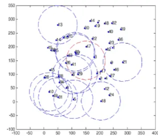
The network topology changes over time due to the mobility between the initial and final states by the algorithms PA2 and PA2-BS as shown in Figures 2 and 3. The sensor transmission ranges are presented by dashed circles. For the seek of clarity, we present only 50 sensors in the network and some transmission ranges. Initially, all the sensors have the same transmission range. Figure 2 presents PA2 algorithm after the first stage run. In order to analyse the sensor behaviour, the sensing field is divided into three regions: high, medium and low population which are coloured respectively in the Figure 2 using gray, white and orange colours. We can see that all the sensors in high population region decrease their transmission range (e.g., sensors: 33, 37, 10 and 49). This can be explained by the fact that these sensors have enough neighbours to improve the area coverage. When the transmission range is reduced, the interference between close sensors is significantly decreased. The sensors in medium and low population region increase (in most cases) their transmission range. Some sensors decrease their transmission range in order to satisfy the two-hop neighbours constraint (e.g. sensors: 31 and 29). In some situations, the sensor keeps its transmission range at maximum to reach the other sensor neighbours (e.g., sensor 13).
Figure 2 MP2-statique (see online version for colours)
At time tk(as shown in Figure 3), the topology of the network
changes whereas the sensors behaviour remains the same. We note that, if two sensors are very close, one of them reduces
its transmission range whereas the second sensor increases its transmission range to reach the others in order to improve the own coverage region (e.g., the sensors: 19 and 40). Note that the coverage of the mobile sensor network does not lie only on the initial configuration, but also on the mobility behaviour of sensors. For these reasons, the PA2 algorithm takes into account, for each sensor, the number of its neighbours that meet the need of its own coverage area.
Figure 3 MP2-mobile (see online version for colours)
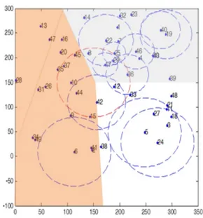
The application of PA2-BS algorithm gives the network topologies presented in Figures 4 and 5. The sensing field is divided into three regions: close, medium and far from the base station which are coloured respectively using grey, white and orange colours. We see that in the two configurations, the sensors that are close to the BS set their transmission ranges to the distance from the BS (e.g. sensors: 12 and 41 in Figure 4 and sensors: 19, 15 and 36 in Figure 5). When the sensors are marginally close to or far from the base station, they reduce their transmission range to reach the needed neighbours (e.g., sensor: 17 and 5 in Figure 4 and sensors: 6, 14 and 36 in Figure 5).
6 Simulations
In order to evaluate the performances of the proposed algorithms, we use the WSnet simulator that is dedicated, especially, to sensor networks.
We compare the obtained results of the proposed algorithms with those of a simple basic solution. In the considered basic solution, the sensors use a static communication range. In other words, in all situations (either the sensor far or near) the sensor transmitted the packets at the maximum power.
In our simulations, we intend to focus on four performance metrics:
• energy consumption • network connectivity
• network lifetime • delivery rate success.
Figure 4 MP2-BS-etatInitial (see online version for colours)
Figure 5 MP2-BS-mobile (see online version for colours)
A. Energy consumption
It is the energy consumed during the transmission, the reception and the idle time. Hence, we use the general formula given in equation (9). Eused= ET x+ ERx+ Eidle+ EM x (9) Eused−total= n ∑ i=0 Eusedi (10)
where the superscript i indicate the sensor i and n the number of neighbour sensors.
B. Network connectivity
The wireless sensor network connectivity is defined as the connectivity of the largest connected component. Hence, it can reflect the network connectivity status and throughput. It can provide reliable evidence for the timely adjustment of the network topology (Gu and Feng, 2010). Consequently, the network connectivity (NC) is calculated as follow:
N C = Biggest connected component size
Network size (11)
C. Network lifetime
The definition of network lifetime is the time span from the deployment to the instant when the network is considered non-operational. A network is considered non-operational according to the chosen application. It may be, for example, the instant when the first sensor dies, a percentage of dead sensors, the network connectivity is lost, or the loss of coverage occurs. In our study, we consider the case of the percentage of dead sensors (Chen, 2005). Thus, if the number of dead sensors is greater than 80%, we assume that the network is non-operational.
D. Packet delivery success rate
In all WSN applications, the packet delivery success rate (PDR) is very important in order to accomplish the network task. Since, in the simulations we evaluate the packet delivery success rate defined as:
PDR = Number of received packets
Number of sent packets (12)
6.1 Parameters and environment
In our simulations, different network sizes are considered: 200, 400, 600 and 800 nodes in order to assess its impact on the network performances. The sensors are distributed randomly in a square area of 300× 300 m. A single and stationary base station is used. It is located in the centre of the area. The sensors move randomly with speed varying between 1 m/s and 30 m/s. The complete configuration is summarised in Table 1.
Table 1 Simulation parameters
Parameters Values
Area size 300 m× 300 m
Simulation duration 7200 s
Number of sensors 200, 400, 600 and 800
Max transmission power 0 dBm
Min transmission power –25 dBm
Max transmission range 200 m
Max speed of sensors 30 m/s
6.2 Results
6.2.1 Energy consumption
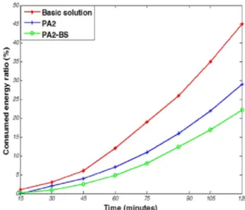
Figure 6 shows the ratio of the consumed energy over the simulation time. We can see that PA2-BS outperforms the PA2
and the basic solution by almost 15% for 90 min and more than 30% for 120 min. This can be explained, on one hand by the decrease of transmission power according to the nearest two-hop neighbours which consume less energy and on the other hand by the decrease of the transmission power of the sensors that are close to the BS. As expected, the improvement of performance due to the use of PA2-BS solution compared to the PA2 and the basic solution is more emphasised for a long-run simulation. The reason is that all the sensors use, initially, the same transmission power. Consequently, the difference of consumed energy is not important in the beginning of the experimentation.
Figure 6 Consumed energy vs. simulation time (600 nodes)
To evaluate the quality of the proposed algorithms in a mobile environment, we compare the consumed energy to the solutions in Figure 7. For 400 sensors, we can observe that the consumed energy increases according to the sensors speed. However, with the PA2-BS, sensors consume considerable less energy compared with the two solutions. This is due to the reduction of transmission power.
Figure 8 presents the consumed energy for different network densities. We can see that the difference of the consumed energy for small network (200 sensors) is not significant. This can be explained by the dispersion of sensors in the area which increases the distances between neighbours and the distance between the sensors and the BS. Thus, the sensors cannot decrease their transmission power. Nevertheless, for large-scale networks (more than 200 sensors), it is clear that PA2-BS outperforms the two solutions by 17% for 600 sensors and by almost 40% for 800 sensors. This means that PA2-BS is able to save more energy for large-scale WSN.
Figure 8 Consumed energy vs. the number of sensors (Time 5400 s)
6.2.2 Network connectivity
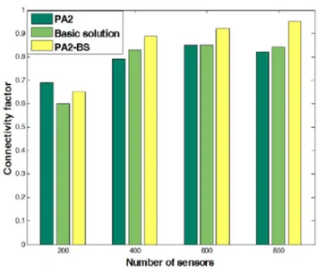
In order to evaluate the performance of the proposed algorithms in terms of connectivity, we calculate the number of connected components with different densities. Figure 9 shows that PA2-BS can manage, in a better way, the consumed energy without adversely affecting the connectivity of the network. However, PA2 has almost the same connectivity than the basic solution. This can be explained by the variations of transmission power which respect the number of neighbours and the distance from BS. This way, despite the mobility of nodes, we always keep the connectivity of the network.
6.2.3 Network lifetime
We assume that the network lifetime is defined as the moment in time when the network is not connected anymore because the failure of one or more sensors. We observe in Figure 10 the impact of the variation of transmission power on the performance of PA2-BS, according to the distance between its neighbours on two-hop. and the distance from BS. For all configurations, the network lifetime using PA2-BS is better than the two other solutions. This is justified by the results depicted on Figure 8 in which we can note that PA2-BS saves more energy and allows the network to operate longer. Hence, PA2-BS improves network lifetime.
Figure 9 Connectivity factor vs. number of sensors
Figure 10 Network lifetime vs. number of sensors (see online version for colours)
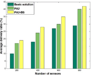
6.2.4 Packet delivery success rate
We can note in Figure 11 that, for all configurations, the PA2-BS ensures a good delivery ratio compared to the two other solutions. We conclude that MP2-BS is able to save energy without adversely affecting the quality of communications. It exists a proportional relationship between the transmission power and the interferences. So, when the transmission power decreases, the interferences decrease. Consequently, the number of packets properly delivered increases.
7 Conclusions
We have presented two power allocation algorithms for mobile sensor networks. These algorithms are designed to develop an effective mechanism to improve the energy conservation, while simultaneously constraining the connectivity. The first proposed algorithm PA2 is based on the self-regulation of
transmission power, for each sensor, according to the distance with its two-hop neighbours. The enhanced proposed PA2-BS algorithm is based on the same principle than the PA2 and in addition it considers the distance between the sensors and the BS. Using this combination, the energy consumption is decreased for every sensor and the connectivity is maintained with the required number of neighbours.
Figure 11 Delivery ratio vs. number of sensors (see online version for colours)
We have evaluated these algorithms by running an extensive set of simulations. Starting by a configuration in which all the sensors has the same transmission range, the PA2 and PA2-BS algorithms provide promising results both in terms of increased packet delivery rate and extended network lifetime without adversely affecting the network connectivity.
In the future, we plan to implement the proposed algorithms in a test-bed environment in order to perform a more accurate evaluation.
References
Alavi, M., Walsh, M. and Hayes, M.J. (2009) ‘Robust distributed active power control technique for IEEE 802.15.4 wireless sensor networks: a quantitative feedback theory approach’,
Control Engineering Practice, 2009 Elsevier International journal, Vol. 17, No. 7, pp.805–814.
Al-Karaki, J.N. and Kamal, A.E. (2004) ‘Routing techniques in wireless sensor networks: a survey’, Wireless Communication,
2004 IEEE International Journal on, Vol. 11, No. 6, pp.6–28.
Ammari, H. and Mulligan, R. (2010) ‘Coverage in wireless sensor networks: A survey’, Network Protocols and Algorithms, 2010
International Journal on, Vol. 2, pp.27-53.
Chamam, A. and Pierre, S. (2009) ‘On the planning of wireless sensor networks: energy-efficient clustering under the joint routing and coverage constraint’, Mobile Computing, 2009 IEEE
Transaction on, Vol. 8, No. 8, pp.1077–1086.
Chang, R. and Kuo, C. (2006) ‘An energy efficient routing mechanism for wireless sensor networks’, Advanced Information Networking and Applications (AINA), 2006 20th International Conference on, pp.308–312.
Chen, Y. (2005) ‘On the lifetime of wireless sensor networks’,
Communication, 2005 IEEE lettres, pp.976–978.
Correia, H.A., Macedo, D., dos Santos, A., Loureiro, A.F., Nogueira, J. and Marcos, S. (2007) ‘Transmission power control techniques for wireless sensor networks’, Computer Networks ,
2007 International Journal on, Vol. 51, No. 17, pp.4765–4779.
Djemili Tolba, F., Magoni, D. and Lorenz, P. (2007a) ‘Saving energy and maximizing connectivity by adapting transmission range in 802.11g MANETs’, Communications Software and Systems,
2007 International Journal on, Vol. 3, No. 2, pp.81–89.
Djemili Tolba, F., Magoni, D. and Lorenz, P. (2007b) ‘Connectivity, energy and mobility driven clustering algorithm for mobile ad hoc networks’, (GLOGECOM), 2007 IEEE Global
Communication Conference, pp.2786–2790.
Ekici, E., Gu, Y. and Bozdag, D. (2006) ‘Mobility-based communication in wireless sensor networks’, Communications,
2006 IEEE Magazine, Vol. 44, No. 7, pp.56–62.
Fleury, E. and Simplot-Ryl, D. (2009) Réseaux de capteurs: théorie
et modélisation, Hermes Science, 2009 Lavoisier.
Ghosh, S., Singh, S., Veeraraghavan, P. and Zhang, L. (2009) ‘Performance of a wireless sensor network MAC protocol with a global sleep schedule’, Multimedia and Ubiquitous
Engineering, 2009 International Journal on, Vol. 4, No. 2,
pp.99–114.
Gu, X. and Feng, H. (2010) ‘Connectivity analysis for a Wireless sensor network based on percolation theory’,
Computer Application and System Modeling (lCCASM), 2010 International Conference on, pp.203–207.
Hackmann, G., Chipara, O. and Lu, C. (2008) ‘Robust topology control for indoor wireless sensor networks’, Embedded
networked sensor systems (SenSys), 2008 International Conference on, pp.57–70.
Heinzelman, W., Chandrakasan, A. and Balakrishnan, H. (2000) ‘Energy-efficient communication protocols for wireless microsensor networks (leach)’, Systems Science, 2000 the 33rd
Hawaii International Conference on, pp.3005–3014.
Hoene, C. and Gunther, A. (2005) ‘Measuring round trip times to determine the distance between wlan nodes’, Networking, 2005
International Conference on, pp.768–779.
Jiuqiang, X., Liu, W., Lang, F., Zhang, Y. and Wang, C. (2010) ‘Distance Measurement Model Based on RSSI in WSN’,
Wireless Sensor Network, 2010 International Journal on, Vol. 2,
No. 4, pp.600–611.
Keshavarzian, A., Huang, L. and Lakshmi, V. (2006) ‘Wakeup scheduling in wireless sensor networks’, Mobile Ad Hoc
Networking and Computing (MobiHoc), 2006 7th ACM International Symposium on, pp.322–333.
Kubisch, M., Karl, H., Wolisz, A., Zhong, L.C. and Rabaey, J. (2003) ‘Distributed algorithms for transmission power control in wireless sensor networks’, Wireless Communications and
Networking (WCNC), 2003 IEEE International Conference on,
pp.558–563.
Lai, C., Hwang, D., Pete, S. and Bo-Cheng, K. (2004) ‘Reducing radio energy consumption of key management protocols for wireless sensor networks’, Low Power Electronics and Design
(ISLPED), 2004 International Symposium on, pp.351–356.
Lin, S., Zhang, J., Zhou, G., Gu, L., Stankovic, J.A. and He, T. (2006) ‘ATPC: adaptive transmission power control for wireless sensor networks’, Embedded networked sensor systems (SenSys), 2006
Madsen, T.K., Fitzek, F.H. and Prasad, R. (2004) ‘Impact of different mobility models on connectivity probability of a wireless ad hoc network’, Wireless Ad-Hoc Networks, 2004 International
Conference on, pp.120–124.
Navidi, W. and Camp, T. (2004) ‘Stationary distributions for the random waypoint mobility model’, Mobile Computing, 2004
IEEE Transaction on, Vol. 3, No. 1, pp.99–108.
Pantazis, N.A., Vergados, D. and Douligeris, C. (2009) ‘Energy efficiency in wireless sensor networks using sleep mode TDMA scheduling’, Ad Hoc Networks, 2009 International Journal on, Vol. 7, No. 2, pp.322–343.
Qiao, D., Yang, G., Tong, B. and Zhang, W. (2008) ‘Sensor-aided overlay deployment and relocation for vast-scale sensor networks’, Computer Communications (INFOCOM), 2008 27th
IEEE International Conference on, pp.2216–2224.
Simarpreet, K. and Mahajan, L. (2011) ‘Power saving MAC protocols for WSNs and optimization of S-MAC protocol’,
Radio Frequency Identification and Wireless Sensor Networks, 2011 International Journal on, Vol. 1, No. 1, pp.1–8.
Songz, Y., Shue Chen, C. and Liyz, Y. (2008) ‘An exploration of geographic routing with k-hop based searching in wireless sensor networks’, Communications and Networking in China
(ChinaCom), 2008 International Conference on, pp.376–381.
Sukhatme, G. and Poduri, S. (2004) ‘Constrained coverage for mobile sensor networks’, Robotics and Automation (ICRA), 2004 IEEE
International Conference on, pp.165–171.
Tonguz, O. and Ferrari, G. (2006) Ad Hoc Wireless Networks – A
Communication-Theoretic Perspective, John & Wiley, pp.1–3.
Wen jing, H., Pan, Y., Kok, P. and Loh, K. (2009) ‘Performance evaluation of efficient and reliable routing protocols for fixed power sensor networks’, Wireless Communications, 2009 IEEE
Transaction on, Vol. 8, No. 5, pp.2328–2335.
Weng, C.C., Chen, C.W. and Ku, C.J. (2011) ‘A minimum transmission energy consumption routing protocol for user-centric wireless networks’, System Integration (SII), 2011 IEEE
International Symposium on, pp.1143–1148.
Witheephanich, K., Escaano, J. and Hayes, M. (2010) ‘Explicitly constrained generalised predictive control strategies for power management in ambulatory wireless sensor network systems’,
American Control (ACC), 2010 Conference, pp.1856–1861.
Zhao, Y., Wu, J., Li, F. and Lu, S. (2010) ‘VBS: maximum Lifetime sleep scheduling for wireless sensor networks using virtual backbones’, Computer Communications (INFOCOM), 2010