Pépite | Caractéristiques avancées pour la représentation d’images : intégration des relations, des poids, de la profondeur, et du temps

Texte intégral

(1)HDR de Jean Martinet, Lille 1, 2016. ` DIRIGER DES RECHERCHES HABILITATION A Discipline : Informatique. Advanced features for image representation: integrating relations, weights, depth, and time Jean Martinet. Mémoire préparé au sein de l’équipe FOX de CRIStAL, et soutenu publiquement le 15 décembre 2016 Jury : Philippe Joly ńot Georges Que Nicu Sebe Liming Chen Ichiro Ide Joemon Jose Olivier Colot Chaabane Djeraba. Professeur DR CNRS Professeur Professeur Professeur Professeur Professeur Professeur. Université Toulouse 1 Capitole Université Grenoble Alpes Università degli Studi di Trento, Italie Ecole Centrale de Lyon University of Nagoya, Japon University of Glasgow, Royaume-Uni Université Lille 1 – Sciences et Technologies Université Lille 1 – Sciences et Technologies. Rapporteur Rapporteur Rapporteur Examinateur Examinateur Examinateur Président Garant. Numéro d’ordre: 42290. © 2016 Tous droits réservés.. doc.univ-lille1.fr.

(2) HDR de Jean Martinet, Lille 1, 2016. Acknowledgements This document describes my research activities during the last 15 years. Research is a collaborative process, and it is my pleasure to thank all the persons who contributed to this work. First of all, I would like to warmly thank all jury members for accepting to evaluate my work, and for taking time to travel to Lille to attend the defence; I specifically want to thank the reviewers, Philippe Joly, Georges Quénot, and Nicu Sebe, for writing a report, in addition to carefully reading my habilitation thesis. I thank Olivier Colot for participating to the jury, and for taking on the role of the President of the jury. I would like to thank Chaabane Djeraba for his support and guidance along the years, and for trusting me. I specially thank all students and colleagues involved in this work. I also thank all members (present and past) of FOX team, IRCICA, CRIStAL, and IUT A for sharing the everyday life at work. I wish to thank Mohamed Daoudi, Ludovic Macaire, and Nicolas Anquetil for the useful proofreading. Finally, I am happy to thank my family and especially my dear mother for being extremely supportive. I send a special thank to Fátima for her helpful dedication, Nilo for his encouraging smiles and songs, and Luna for urging me to finish, though she won the race when showing up a month in advance – exactly the time that I needed to finish writing up :-) But hey, life is life and there is always space to welcome a kid at home.. © 2016 Tous droits réservés.. doc.univ-lille1.fr.

(3) HDR de Jean Martinet, Lille 1, 2016. ii. © 2016 Tous droits réservés.. doc.univ-lille1.fr.

(4) HDR de Jean Martinet, Lille 1, 2016. Abstract Tremendous amounts of visual data are produced every day, such as user-generated images and videos from social media platforms, audiovisual archives, etc. It is important to be able to search and retrieve documents among such large collections. Our work in computer vision and multimedia information retrieval focuses on visual features for image representation. In particular, inside the entire processing chain ranging from visual data acquisition with sensors to the user interface that facilitates the interaction with the system, our research addresses the internal representation of visual data in the form of an index that serves as a reference for the system regarding the image contents. In the general context of image representation, we describe in a first part some contributions related to the widely-used paradigm of “bags of visual words”. We also discuss the general notion of relation, taken at several levels – the low level of visual words, the transversal level aiming for cross-modal annotation, and the high level of semantic objects. Finally, we focus on the definition of weighting models, that serve as visual counterparts to popular weighting schemes used for text. Because of the specificity of persons and their faces compared to general objects, we focus in a second part on specific features and methods for person recognition. Two directions are developed to overcome some limitations of static 2D approaches based on face images, with the objective of improving systems’ precision and robustness. One direction integrates depth in facial features, and the other takes advantage of temporal information in video streams. In both cases, dedicated features and strategies are investigated. Keywords: Computer vision, Multimedia information retrieval, Image representation, Indexing, Visual features, Weighting scheme, Person recognition.. © 2016 Tous droits réservés.. doc.univ-lille1.fr.

(5) HDR de Jean Martinet, Lille 1, 2016. iv. © 2016 Tous droits réservés.. doc.univ-lille1.fr.

(6) HDR de Jean Martinet, Lille 1, 2016. R´ esum´ e D’immenses quantités de données visuelles sont générées tous les jours, telles que les images et vidéos produites par les utilisateurs des réseaux sociaux, les archives audiovisuelles, etc. Il est important de pouvoir chercher et retrouver des documents au sein de tels grands volumes de données. Notre travail en vision par ordinateur et recherche d’information multimédia porte sur les caractéristiques visuelles pour la représentation d’images. En particulier, dans la chaˆıne des traitements allant de l’acquisition des données visuelles via des capteurs jusqu’à l’interface utilisateur qui facilite l’interaction avec le système, notre recherche s’intéresse à la représentation interne des données visuelles sous la forme d’un index qui sert de référence pour le système concernant le contenu des images. Dans le contexte général de la représentation d’images, nous décrivons dans une première partie quelques contributions liées au paradigme populaire des “sacs de mots visuels”. Nous discutons également la notion générale de relation, prise à différents niveaux – le bas niveau des mots visuels, le niveau transverse qui vise l’annotation intermodale, et le haut niveau des objets sémantiques. Finalement, nous nous attachons à définir des modèles de pondération, qui servent de pendants visuels des schémas de pondération utilisés pour le texte. En raison de la spécificité des personnes et visages en comparaison aux objets généraux, nous nous intéressons dans une seconde partie aux caractéristiques et méthodes spécifiques pour la reconnaissance de personnes. Deux directions sont développées pour pallier certaines limitations des approches 2D statiques basées sur des images de visages, avec l’objectif d’améliorer la précision et la robustesse des systèmes. L’une des directions intègre la profondeur dans les caractéristiques faciales, et l’autre exploite l’information temporelle dans les flux vidéo. Dans les deux cas, des caractéristiques et stratégies dédiées sont étudiées. Mots-cl´ es : Vision par ordinateur, Recherche d’information multimédia, Représentation d’images, Indexation, Caractéristiques visuelles, Schéma de pondération, Reconnaissance de personnes.. © 2016 Tous droits réservés.. doc.univ-lille1.fr.

(7) HDR de Jean Martinet, Lille 1, 2016. vi. © 2016 Tous droits réservés.. doc.univ-lille1.fr.

(8) HDR de Jean Martinet, Lille 1, 2016. © 2016 Tous droits réservés.. doc.univ-lille1.fr.

(9) HDR de Jean Martinet, Lille 1, 2016. Contents Contents. ii. List of Figures. iv. List of Tables. viii. 1 Introduction 1.1 Motivations . . . . . . . . . . . . . . . . . . . . . . . . . . . . . . . . . . . . . 1.2 Main contributions and overview . . . . . . . . . . . . . . . . . . . . . . . . . 2 Image representations: visual vocabularies, relations, and weights 2.1 Bag of visual words . . . . . . . . . . . . . . . . . . . . . . . . . . . . 2.1.1 Discriminative descriptor for bag of visual words . . . . . . . . 2.1.2 Iterative vocabulary selection based on information gain . . . 2.1.3 Split representation for mobile image search . . . . . . . . . . 2.1.4 Textual vs. visual words . . . . . . . . . . . . . . . . . . . . . 2.2 Relations between descriptors . . . . . . . . . . . . . . . . . . . . . . 2.2.1 Visual phrases taken as mid-level descriptors . . . . . . . . . . 2.2.2 Cross-modal relations for image annotation . . . . . . . . . . . 2.2.3 Integrating term relations into the vector space model . . . . . 2.3 Weighting models for image parts . . . . . . . . . . . . . . . . . . . . 2.3.1 Spatial weighting scheme for visual words . . . . . . . . . . . 2.3.2 Gaze-based region importance . . . . . . . . . . . . . . . . . . 2.3.3 Geometry-based weighting model for image objects . . . . . . 2.3.4 Weighting scheme for star graphs . . . . . . . . . . . . . . . . 2.4 Conclusion . . . . . . . . . . . . . . . . . . . . . . . . . . . . . . . . .. 1 1 2. . . . . . . . . . . . . . . .. 7 9 9 12 16 22 23 25 28 30 38 39 40 42 49 51. 3 Person recognition: exploring depth and time 3.1 Face recognition by combining visual and depth data . . . . . . . . . . . . . . 3.1.1 Depth map generation with stereo cameras . . . . . . . . . . . . . . . . 3.1.2 DLBP: Depth Local Binary Patterns . . . . . . . . . . . . . . . . . . .. 55 59 59 67. . . . . . . . . . . . . . . .. . . . . . . . . . . . . . . .. . . . . . . . . . . . . . . .. . . . . . . . . . . . . . . .. ii. © 2016 Tous droits réservés.. doc.univ-lille1.fr.

(10) HDR de Jean Martinet, Lille 1, 2016. CONTENTS. 3.2. 3.3. 3.1.3 Two-stage fusion of 2D and 3D modalities . . . . . . . 3.1.4 FoxFaces multi-purpose dataset . . . . . . . . . . . . . Dynamic person recognition in TV shows . . . . . . . . . . . . 3.2.1 Problem formulation . . . . . . . . . . . . . . . . . . . 3.2.2 Space-time histograms . . . . . . . . . . . . . . . . . . 3.2.3 Persontrack clustering for re-identification . . . . . . . 3.2.4 Frame-based persontrack identification . . . . . . . . . 3.2.5 Cluster labeling . . . . . . . . . . . . . . . . . . . . . . 3.2.6 What can be done when using only 0.1% of the frames? 3.2.7 FoxPersonTracks benchmark for re-identification . . . . Conclusion . . . . . . . . . . . . . . . . . . . . . . . . . . . . .. . . . . . . . . . . .. . . . . . . . . . . .. . . . . . . . . . . .. . . . . . . . . . . .. . . . . . . . . . . .. . . . . . . . . . . .. . . . . . . . . . . .. . . . . . . . . . . .. . 75 . 80 . 84 . 86 . 88 . 90 . 93 . 98 . 101 . 101 . 105. 4 Conclusion 107 4.1 Summary of contributions . . . . . . . . . . . . . . . . . . . . . . . . . . . . . 107 4.2 Impact . . . . . . . . . . . . . . . . . . . . . . . . . . . . . . . . . . . . . . . . 110 4.3 Future work . . . . . . . . . . . . . . . . . . . . . . . . . . . . . . . . . . . . . 111 5 Curriculum Vitæ 5.1 General details . . . . . . . . . . . . . . . . 5.2 Career . . . . . . . . . . . . . . . . . . . . . 5.3 Research directions . . . . . . . . . . . . . . 5.4 Teaching activities since 2013 . . . . . . . . 5.5 PhD students supervision . . . . . . . . . . 5.6 Research projects, relation with industry . . 5.7 Other activities and contributions . . . . . . 5.8 Selected publications between 2008 and 2016 References. . . . . . . . .. . . . . . . . .. . . . . . . . .. . . . . . . . .. . . . . . . . .. . . . . . . . .. . . . . . . . .. . . . . . . . .. . . . . . . . .. . . . . . . . .. . . . . . . . .. . . . . . . . .. . . . . . . . .. . . . . . . . .. . . . . . . . .. . . . . . . . .. . . . . . . . .. . . . . . . . .. . . . . . . . .. 115 115 115 116 116 116 117 118 118 123. iii. © 2016 Tous droits réservés.. doc.univ-lille1.fr.

(11) HDR de Jean Martinet, Lille 1, 2016. List of Figures 1.1. Overview of the work presented in this document. . . . . . . . . . . . . . . . .. 2.1. Extraction of the edge context descriptor in the 2D spatial space, after clustering the points in the 5-dimensional color-spatial feature space with a GMM. . . . . Comparison of the precision obtained with the proposed descriptor and with SURF taken alone, with different vocabulary sizes. . . . . . . . . . . . . . . . . KMeans-based vocabulary versus random selection of words. . . . . . . . . . . Iterative selection scores; the initial vocabulary size is 2048. . . . . . . . . . . Mean scores for several initial vocabulary sizes, from 1024 to 65536. . . . . . . Illustration of the mobile image search scenario. . . . . . . . . . . . . . . . . . Elementary blocks of Les Invalides. (a) SIFT keypoints are represented by colored dots; each color corresponds to a cluster. (b) Each row contains 25 sample patches from a given cluster. Best seen in color. . . . . . . . . . . . . . . . . . Assignment of elementary block eB0 to visual words C0 , C1 , and C2 . . . . . . . Assignment of eBi to Cj to estimate the associated visual word histogram. . . (a) Word distribution from Wikipedia entries in November 2006 in a log-log plot (Source: Wikipedia). (b) Zipf’s law and Luhn’s model. . . . . . . . . . . Word distributions for Caltech-101. A similar tendency is observed with Pascal VOC2012. . . . . . . . . . . . . . . . . . . . . . . . . . . . . . . . . . . . . . . Syntactic granularity in an image and a text document. . . . . . . . . . . . . . Example of representation of two rules. The upper representation shows a high confidence rule, and the lower representation shows a lower confidence rule. Only the support of Y is changed between the two cases. . . . . . . . . . . . . Example of a visual phrase corresponding to faces, made of strongly correlated visual words. Best seen in color. . . . . . . . . . . . . . . . . . . . . . . . . . . Comparison of the classification precision for SVWs, SVPs, and their combination, and also the classical visual words. . . . . . . . . . . . . . . . . . . . . . Comparison of the classification precision for the proposed and two other stateof-the-art approaches. . . . . . . . . . . . . . . . . . . . . . . . . . . . . . . . .. 2.2 2.3 2.4 2.5 2.6 2.7. 2.8 2.9 2.10 2.11 2.12 2.13. 2.14 2.15 2.16. 3 11 12 14 15 15 17. 18 19 20 23 24 25. 27 28 29 29. iv. © 2016 Tous droits réservés.. doc.univ-lille1.fr.

(12) HDR de Jean Martinet, Lille 1, 2016. LIST OF FIGURES 2.17 Example of multimedia stream containing two modalities. Objects are represented with orange boxes inside the modalities, and relations between them are shown (plain line: intra-modal, same temporal window ; dashed line: intramodal, neighbour windows ; dotted: cross-modal, same window). . . . . . . . . 2.18 Star graphs of unary, binary and ternary relations (from left to right). . . . . . 2.19 Example of two images likely to be labeled with “Jean”, “Matthieu”, “Boat”, and “Sky”. While these four labels do not make it possible to distinguish between these images, the star graphs given Figure 2.18 help differentiating them since they describe only the left image. . . . . . . . . . . . . . . . . . . . . . . . . . 2.20 General outline of the star graph lattice. . . . . . . . . . . . . . . . . . . . . . 2.21 Vector of the document before (left) and after (right) the document expansion. 2.22 From concepts to star graphs: impact of integrating the relations. Above: Coll-1, below: Coll-2. . . . . . . . . . . . . . . . . . . . . . . . . . . . . . . . . . . . . 2.23 Result for the subset of 12 relational queries of Coll-2. . . . . . . . . . . . . . . 2.24 Recall-precision curves for best-performing settings of each system (Left: Coll-1, Right: Coll-2). . . . . . . . . . . . . . . . . . . . . . . . . . . . . . . . . . . . . 2.25 Comparison between the spatial weighting approach performance with the original bag of visual words. . . . . . . . . . . . . . . . . . . . . . . . . . . . . . . 2.26 Example of images displaying gaze points (yellow), and showing the processed clusters as superimposed disks (pink), with their estimated importance denoted by the size of the disks. Best seen in color. . . . . . . . . . . . . . . . . . . . . 2.27 16 typical configurations for an IO represented by the disk. . . . . . . . . . . . 2.28 Example of photos showing configurations 2 (left) and 8 (right) of Figure 2.27. 2.29 Recall-precision graph for the global color histogram matching, the IO matching with a Boolean weighting scheme, and the IO matching with the proposed weighting scheme – with and without the idf component. The graph also displays the result of a text-based keyword search. . . . . . . . . . . . . . . . . . 2.30 Divergence values for all query terms. . . . . . . . . . . . . . . . . . . . . . . . 2.31 Retrieval results with several weighting schemas for the two collections, in the original space and the extended space. Above: Coll-1, below: Coll-2. S refers to the Size criterion, and P refers to the Position criterion. . . . . . . . . . . . . 3.1 3.2. 3.3. 3.4. Example of appearance variation of a face. . . . . . . . . . . . . . . . . . . . . Effects of changes in acquisition conditions: (a) frontal pose, (b) pose change, (c) light change. Each line shows a different face, however faces in each column look more similar one to another. . . . . . . . . . . . . . . . . . . . . . . . . . Stereo cameras setting. p is a point in the 3D real world with corresponding projections pg and pd in the left and right images, respectively. f is the camera focal, and b is the baseline. . . . . . . . . . . . . . . . . . . . . . . . . . . . . . Illustration of the aperture problem for homogeneous face regions: it is hard to find matching points. . . . . . . . . . . . . . . . . . . . . . . . . . . . . . . . .. 30 32. 33 33 34 35 36 37 41. 43 45 45. 46 48. 52 56. 57. 61 61. v. © 2016 Tous droits réservés.. doc.univ-lille1.fr.

(13) HDR de Jean Martinet, Lille 1, 2016. LIST OF FIGURES 3.5 3.6 3.7 3.8. 3.9 3.10 3.11 3.12 3.13 3.14. 3.15 3.16 3.17 3.18 3.19. 3.20 3.21. 3.22 3.23 3.24 3.25 3.26. 3.27. Construction of the disparity model for a face. . . . . . . . . . . . . . . . . . . Decomposition of the disparity model into slices. . . . . . . . . . . . . . . . . . Examples of model projection on a face with different poses. . . . . . . . . . . (a) Detection of cut points to split a depth row into segments. Red dots show cut points. (b) Noisy segments detection. The mi values are the mean values of Si segments. . . . . . . . . . . . . . . . . . . . . . . . . . . . . . . . . . . . . . Depth map denoising: (a) depth map with holes, (b) gradient, (c) noisy slice detection, (d) corrected depth map. . . . . . . . . . . . . . . . . . . . . . . . . Example of depth maps: (a) original (ground truth), (b) our method, (c) graphcut and (d) block-matching. . . . . . . . . . . . . . . . . . . . . . . . . . . . . Comparison of depth maps. Left: RMS values. Centre: PBM values. Right: Processing time. . . . . . . . . . . . . . . . . . . . . . . . . . . . . . . . . . . . Examples of shape patterns detected with LBP1,8 . . . . . . . . . . . . . . . . . Confusion between similar 3D shapes. (a) LBP codes. (b) Potential 3D shape matches. . . . . . . . . . . . . . . . . . . . . . . . . . . . . . . . . . . . . . . . Extraction of the DLBP descriptor from local histograms extracted from the sign and magnitude matrices with H = 2 × 2: (a) depth map, (b) sign matrix, (c) magnitude matrix, (d) resulting histogram. . . . . . . . . . . . . . . . . . . Impact of varying the radius R on the precision of recognition (H = 25). . . . Impact of varying the number H of local histograms to build DLBP vectors. . Comparison of LBP, 3DLBP, and DLBP. . . . . . . . . . . . . . . . . . . . . . Overview of the proposed two-stage fusion strategy for bimodal 2D-3D face recognition. . . . . . . . . . . . . . . . . . . . . . . . . . . . . . . . . . . . . . Comparison between several face recognition methods: monomodal 2D, monomodal 3D, early fusion, late fusion, and the proposed two-stage fusion strategy, for the five collections. . . . . . . . . . . . . . . . . . . . . . . . . . . Examples showing some illumination variations in FRGC dataset (top row) and Texas dataset (bottom row). . . . . . . . . . . . . . . . . . . . . . . . . . . . . Sample images from the 3 sensors. Top row: infrared sensor images from Kinect: (a) color (b) depth. Middle row: time-of-flight sensor images from SR4000: (a) infrared (b) depth (c) confidence matrix (bright pixels mean high confidence). Bottom row: image triple from the stereo camera Bumblebee XB3. . . . . . . . Example of all possible variations for a subject: (a) 3 lighting conditions (b) 7 face expressions (c) 30 head poses. . . . . . . . . . . . . . . . . . . . . . . . . . Annotated interest points on a face. . . . . . . . . . . . . . . . . . . . . . . . . Global illustration of the proposed system for person recognition in video streams. Actual example of a persontrack. . . . . . . . . . . . . . . . . . . . . . . . . . Evolution of the precision as the number of bins in the descriptors increases, from 10 to 10,000 bins. Plots for color histograms and spatiograms are superimposed. . . . . . . . . . . . . . . . . . . . . . . . . . . . . . . . . . . . . . . . Evolution of the precision as the memory cost increases for each approach. . .. 63 64 64. 65 66 67 67 69 69. 72 73 74 76 77. 79 80. 81 82 83 85 87. 92 93. vi. © 2016 Tous droits réservés.. doc.univ-lille1.fr.

(14) HDR de Jean Martinet, Lille 1, 2016. LIST OF FIGURES 3.28 Precision Pp w.r.t. the number of frames used and the strategy considered to identify the persontracks. The score for random sampling is averaged over 100 runs. . . . . . . . . . . . . . . . . . . . . . . . . . . . . . . . . . . . . . . . . . 3.29 Sample frames taken from a debate show illustrating a specific journalist behaviour: the journalist introduces the subject (frontal pose), then asks a question to one of the guests (non-frontal pose). . . . . . . . . . . . . . . . . . . . . . . 3.30 Precision of recognition Pp w.r.t. the ratio of seed persontracks used to identify the persontracks, using (left) random selection (center) similarity-based selection and, (right) confidence score-based selection. . . . . . . . . . . . . . . . . 3.31 Steps for building FoxPersonTracks dataset from the REPERE dataset. . . . . 3.32 Example of person extraction process on a single frame and a single person. Left: Original frame with the detected face. Center: Mask calculated from the detected face. Right: Result of the Grabcut algorithm applied on the original image using the mask. . . . . . . . . . . . . . . . . . . . . . . . . . . . . . . . 3.33 (a) Number of occurrences per identity distribution in the dataset ranging from 1 to 278 (x-axis) with an average of 17. (b) Duration in frames distribution of our datasets ranging from 7 frames to 896 frames (x-axis) with an average of 55 frames. Note that the y-axis is logarithmic. . . . . . . . . . . . . . . . . . .. 97. 98. 100 103. 104. 105. vii. © 2016 Tous droits réservés.. doc.univ-lille1.fr.

(15) HDR de Jean Martinet, Lille 1, 2016. List of Tables 2.1 2.2. Running time (in seconds) of KMeans with NeB = α × ND . . . . . . . . . . . . 20 mAP (in %) on Paris, Oxford and Holidays datasets for a standard approach (baseline), a vocabulary with randomly sampled descriptors, and our method using different values of NeB , NC . Results above the baseline are shown in bold. 21. 3.1 3.2. Baseline performance of the re-identification method [AMT15]. . . . . . . . . . 96 Precision and recall of the standard recognition framework and the proposed approach based on intra-persontrack propagation. All the frames of the dataset are used. . . . . . . . . . . . . . . . . . . . . . . . . . . . . . . . . . . . . . . . 97 Results before and after propagating the identity of the persontracks. Propagation is based on majority vote within the clusters. . . . . . . . . . . . . . . . . 100 Comparison of the propagation results of each proposed strategy combinaison using only 1% of the frames of 1% the persontracks of each group. . . . . . . . 102. 3.3 3.4 4.1. Number of publications per topic (related publications), number of citations and average number of citations per year as of October 2016. Source: Google Scholar. . . . . . . . . . . . . . . . . . . . . . . . . . . . . . . . . . . . . . . . 110. viii. © 2016 Tous droits réservés.. doc.univ-lille1.fr.

(16) HDR de Jean Martinet, Lille 1, 2016. Chapter 1 Introduction 1.1. Motivations. In a few decades, the research in multimedia Information Retrieval (IR) and computer vision has reached a very mature state, and yet there are numerous open problems that give the scientific community thrilling challenges. Visual data (images and video) arouse an increasing interest, due to the wide availability of such data, e.g. audiovisual archives, user-generated contents in social media platforms, surveillance, etc. Tremendous amounts of visual data are produced every day, and it is important to be able to search and retrieve documents among large colletions. Visual data gained a major societal importance. Many factors can explain this importance, such as the democratisation of digital cameras (nowadays small and cheap), the low cost of storage, and the generalized access to data networks. For a few examples, in France, there exists over 80 TV channels, meaning that 80 hours of video content are broadcasted every hour. The french INA 1 stores about 70 years of audiovisual archives, representing 300 years of continuous video playing. On YouTube, about 100 hours of video content are uploaded every hour. The core problems in multimedia IR naturally come from those of text IR. The objective is to help users navigate, browse, or search through a multimedia collection. However, contrary to text documents, visual documents do not contain natural semantic evidence such as words or groups of words that can be used to represent their semantic content, and from which they can be retrieved. This fundamental difference between text and visual documents is often referred to as the semantic gap, and has been widely discussed over the last 15 years. This notion was defined by Smeulders et al. [SWS+ 00] as the lack of coincidence between the information that one can extract from the visual data and the interpretation that the same data have for a user in a given situation. This lack of coincidence originates from the difference between the way we perceive visual content and what the machine can extract. 1. Institut National de l’Audiovisuel: National Audiovisual Institute.. 1. © 2016 Tous droits réservés.. doc.univ-lille1.fr.

(17) HDR de Jean Martinet, Lille 1, 2016. In the research presented here, I proposed solutions to overcome some of these problems. This document contains a summary of my research activities spanning from 2002 to 2016, and more specifically at Lille 1 University from 2008. After completing an MSc and a PhD in Computer Science at Grenoble 1 University in 2004, I was awarded a two-year postdoctoral fellowship by the JSPS 1 to visit the National Institute of Informatics in Tokyo (2005-2007). Then I joined Lille 1 University as an Assistant Professor in the FOX 2 research team, that is part of the IMAGE group in CRIStAL 3 laboratory (previously LIFL 4 ).. 1.2. Main contributions and overview. Multimedia IR is a research domain that is intrinsically multi-disciplinary, involving computer vision, pattern recognition, and image processing only for the visual aspects. My research focuses on image representations for objects and persons. Inside the entire processing chain ranging from data acquisition with visual sensors to the user interface that facilitates the interaction with the IR system, my work addresses the internal representation of visual data in the form of an index that serves as a reference for the system regarding the image contents. A timeline of my research activities is given in Figure 1.1, showing the different contributions organized around the topics of image representations (upper part) and person recognition (middle part). For both topics, the figure shows a selection of related conference and journal papers. The lower part indicates my position across the time. These contributions were made possible by the help of many students and colleagues. Figure 1.1 also shows all students involved in the presented work. The contents of Chapter 2 and Chapter 3 describe our work related to image representations and person recognition, respectively. The description is organized by topic rather than chronologically. Image representations (Chapter 2): We describe in Chapter 2 several contributions related to image representations (see the upper part of Figure 1.1). These contributions are in the continuity of my PhD and postdoctoral work, and the PhD of Mr Ismail El Sayad (October 2008 – July 2011), that I co-directed with Prof. Chaabane Djeraba. First, Section 2.1 describes several improvements around the widely-used paradigm of bag of visual words, that consists in representing images or video keyframes using a set of descriptors, that correspond to quantized low-level features. We present an enhanced bag-of-visual-words model that is based on the use of a new descriptor, the Edge Context, that improves the discriminative power by capturing the neighbourhood context of interest points. The Edge Context descriptor has been successfully used as a part of a larger image representation and retrieval model in Ismail’s work. We also introduce two alternative methods to build a visual vocabulary, compared 1. 2. 3. 4.. Japan Society for the Promotion of Science, URL http://www.jsps.go.jp. Fouille et indexation de dOcuments compleXes et multimedia. Centre de Recherche en Informatique, Signal et Automatique de Lille. Laboratoire d’Informatique Fondamentale de Lille.. 2. © 2016 Tous droits réservés.. doc.univ-lille1.fr.

(18) HDR de Jean Martinet, Lille 1, 2016. Figure 1.1 – Overview of the work presented in this document. to the usual KMeans-based quantization of low-level features: (1) an information-gain-based selection process where words are iteratively filtered from a large set of randomly selected descriptors based on their information gain, and (2) a split representation dedicated to mobile image search, where a standard vocabulary is built on the server side; at query time, another query-specific, lightweight vocabulary is built on the client side (mobile device), that forms a compressed representation of the query image to be sent to the server for matching. Finally, a discussion is given about the basis behind adapting and applying text techniques to visual words. Then Section 2.2 discusses the general notion of relation in image representations. In its general definition, a relation refers to the way in which two or more things are connected. In our work, this notion is taken at several levels: (1) low level : we consider relations between visual words in order to discover frequently co-occurring visual words patterns, and to create visual phrases, (2) transversal level : in cases where a multimedia document contains several modalities, we analyze the relations between visual words and other (textual) modalities in 3. © 2016 Tous droits réservés.. doc.univ-lille1.fr.

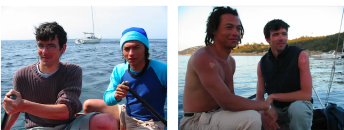
(19) HDR de Jean Martinet, Lille 1, 2016. order to allow cross-modal annotation, and (3) high level : we integrate in the representation model the relations between objects of an image to enrich the semantic representation. Finally, Section 2.3 focuses on the issue of defining a weighting scheme for images. Indeed, since almost half a century, a number of weighting models for text have been designed and widely tested, giving more importance to relevant index terms. It is therefore a mature research domain with generally acknowledged good results. However, defining a weighting model for image is not trivial, because this rises the question of defining a notion of importance for image regions. This section discusses several attempts to define a weighting scheme of image parts at various levels of granularity, that aims to serve as an image counterpart to the tf formulation from the famous tf-idf weighting model [Sal71] used for text. Person recognition (Chapter 3): While Chapter 2 addresses image representations for general objects, this chapter describes our work specifically related to person recognition (see the middle part of Figure 1.1). In image representations, persons – and more specifically their faces, are specific kinds of objects that need dedicated representations. Our objective is to address the limitations of static 2D approaches (i.e. those based on a face picture), that come from the appearance variations due to changes in lighting conditions, viewpoints, pose, and partial occlusions (glasses, hair, beard, etc.). We explored two directions for enhancing the accuracy and robustness of static 2D approaches of person recognition: — the use of depth in face recognition (2D+depth), — and the use of time (2D+time). This work was done during the PhDs of Miss Amel Aissaoui (September 2010 – June 2014) and the PhD of Mr Rémi Auguste (November 2010 – July 2014). In Amel’s work (Section 3.1), we introduced a 2D-3D bimodal face recognition approach that combines visual and depth features in order to provide higher recognition accuracy and robustness than monomodal 2D approaches. First, a 3D acquisition method dedicated to faces is introduced. It is based on a stereoscopic reconstruction using an active shape model to take into account the topology of the face. Then, a novel descriptor named Depth Local Binary Patterns (DLBP) is defined in order to characterize the depth information. This descriptor extends to depth images the standard LBP originally designed for texture description. Finally, a two-stage fusion strategy is proposed, that combines the modalities using both early and late fusion strategies. The experiments conducted with different public datasets, as well as with a new dataset elaborated specifically for evaluation purposes, allowed to validate the three contributions introduced throughout this work. In particular, results showed a high quality for the data obtained using the reconstruction method, and also a gain in precision obtained by using the DLBP descriptor and the two-stage fusion strategy. In Rémi’s work (Section 3.2), we designed a dynamic approach to person recognition in video streams. This approach is dynamic as it benefits from the motion information contained in videos, whereas the static approaches are solely based on still images. The proposed approach is composed of two parts. In the first part, we extract persontracks (short video 4. © 2016 Tous droits réservés.. doc.univ-lille1.fr.

(20) HDR de Jean Martinet, Lille 1, 2016. sequences featuring a single person with no background) from the videos and cluster them with a re-identification method based on a new descriptor: Space-Time Histograms (STH), and its associated similarity measure. The original contribution in this work is the integration of temporal data into the descriptor. Experiments show that it provides a better estimation of the similarity between persontracks than other static descriptors. In the second part of the proposed person recognition approach, we investigate various strategies to assign an identity to a persontrack using its frames, and to propagate this identity to members of the same cluster, based on a standard facial recognition method. Both aspects of our contribution were evaluated using a corpus of real life TV shows broadcasted on BFMTV and LCP TV channels. The experimental results show that the proposed approach significantly improves the recognition accuracy thanks to the use of the temporal dimension both in the STH descriptor and in persontrack identification. Chapter 4 gives a summary of all contributions presented in this document, and opens research perspectives. Finally, an extended curriculum vitæ is provided in Chapter 5.. 5. © 2016 Tous droits réservés.. doc.univ-lille1.fr.

(21) HDR de Jean Martinet, Lille 1, 2016. 6. © 2016 Tous droits réservés.. doc.univ-lille1.fr.

(22) HDR de Jean Martinet, Lille 1, 2016. Chapter 2 Image representations: visual vocabularies, relations, and weights Since the early years of content-based image retrieval in the 1990’s, there has been a great amount of work dedicated to image representations in indexing and retrieval systems. Indeed, a good representation is a needed ground for good IR system performances because the quality of search results highly depends on the quality of the index. This chapter deals with image representations, and it describes our contributions for enhancing such representations. The first part of this chapter, Section 2.1, is related to the widely-used paradigm of bag of visual words – or bag of features, or codebook. This popular approach for representing, searching or categorizing visual documents consists in describing images using a set of descriptors, that correspond to quantized low-level features such as SIFT [Low04] or SURF [BTVG06, BETVG08]. KMeans is the most widely used method for the quantization step. The clusters are used as a codebook where each descriptor is represented by the closest centroid – taken as a visual word, and images are described with visual words 1 . In some situations where e.g. the feature space dimensionality is large, the size of the dataset is large, or the system resources are limited, KMeans can be considered costly or even not feasible. Section 2.1 starts with a description of a new descriptor, the Edge Context, that is a part of our work during the PhD of Ismail El Sayad for defining an enhanced bag-of-visual-words model. This contribution was published at CBMI’10 [ESMUD10a], and in more details in an MTAP journal paper [ESMUD12]. The section also explores two alternative ways to build a visual vocabulary: 1. The first method is an information-gain-based iterative selection process, in a joint work with my colleague Thierry Urruty (University of Poitiers, France) and co-authors. As an alternative to the usual KMeans-based quantization step, this approach consists in randomly selecting a subset of candidates from a large set, and then an iterative process filters out descriptors with the least information gain values until the desired number of features is reached, and considered as visual words forming the vocabulary. This work 1. In this chapter, we refer to this setting as the standard approach.. 7. © 2016 Tous droits réservés.. doc.univ-lille1.fr.

(23) HDR de Jean Martinet, Lille 1, 2016. was published at ICMR’14 [UGL+ 14]. 2. The second contribution consists of a split representation dedicated to mobile image search, in a joint work with my colleagues José Mennesson (Lille 1 University) and Pierre Tirilly (Lille 1 University) during TWIRL project 1 . Despite recent technical advances, mobile devices (smartphones and tablets) still encounter limitations in memory, speed, energy and bandwidth, that represent bottlenecks from mobile image search systems. In the proposed approach, a reference visual vocabulary is built offline and kept on a server. At query time, a “disposable” lightweight vocabulary is built on-the-fly on the mobile device, using only the query image. Descriptors from this specific vocabulary are sent to the server to be matched to the reference vocabulary. The proposed method offers an acceptable tradeoff between the mobile device technical constraints and the search precision. This work was published at ICIP’14 [MTM14]. Section 2.1 ends with a general discussion, published at VISAPP’14 [Mar14], regarding the basis behind adapting and applying text techniques to visual words. Most visual words approaches are inspired from work in text and natural language processing, based on the implicit assumption that visual words can be handled the same way as text words. However, text words and visual words are intrinsically different in their origin, use, semantic interpretation, etc. More specifically, the discussion brings to light the fact that while visual word techniques implicitly rely on the same postulate as in text information retrieval, stating that the words distribution for a natural language globally follows Zipf’s law – that is to say, such words appear in a corpus with a frequency inversely proportional to their rank, this postulate is not always true in the image domain. The second part of the chapter, Section 2.2, discusses the general notion of relation in image representations. While in its general definition, a relation refers to the way in which two or more things are connected, in our work, this notion is taken at several levels: low, transversal, and high levels. — At a low level, we consider the relations beween visual words, and more specifically, how their occurrence patterns can be used to define higher-level descriptors. The idea behind such descriptors originates from the concept of phrases in text indexing and retrieval. For instance, the phrases “dead end”, “hot dog”, or “white house” convey meanings that are different from the same words taken separately. Such phrases can automatically be discovered text corpus analysis with simple statistical tools, and by including them in the indexing vocabulary, the system can benefit from a finer representation. In a similar way, visual words that represent parts of real-world objects tend to co-occur in images in a close neighbourhood: they can be seen as visual phrases. The objective in this work is to build such visual phrases in order to both enrich and refine the image description, and thereby increase the system precision. 1. TWIRL project: June 2012 – October 2014, ITEA 2 Call 5 10029 – Twinning virtual World (on-line) Information with Real world (off-Line) data sources.. 8. © 2016 Tous droits réservés.. doc.univ-lille1.fr.

(24) HDR de Jean Martinet, Lille 1, 2016. — At a transversal level, we analyse cross-modal relations in the context of image annotation. When multimedia documents contain several modalities (i.e. visual, text from optical character recognition or speech transcription), by allowing them to collaborate, the objective is to leverage textual information surrounding image to automatically extract annotations. — At a high level, the relations beween objects in an image can be integrated in the description in order to allow the expression of semantic and spatial relations. For instance, “the dog is sitting in front of the door” is a finer description than just “dog” and “door” for an image. The last part of the chapter, Section 2.3, focuses on the issue of defining a weighting scheme for images, which rises the question of defining a notion of importance for image regions. The purpose of a weighting scheme is to give emphasis to important terms, quantifying how well they semantically describe and discriminate documents in a collection. When it comes to images, the users’ point of view is central for defining weights for image parts in the contexts of retrieval and similarity matching. Like in text retrieval, an image weighting scheme should give emphasis to important regions, quantifying how well they describe documents. The section explores several ways to define a weighting scheme for images.. 2.1. Bag of visual words. The popular bag-of-visual-words approach for representing and searching visual documents consists in describing images using a set of descriptors, that correspond to quantized low-level features. In this section, we start by introducing a descriptor, the Edge Context, that is a part of an enhanced bag of visual words model. Then we describe two non-standard ways to build vocabularies. Finally, we discuss the very notion of visual word, and the application of text processing techniques (e.g. word filtering, weighting, etc.) to such words.. 2.1.1. Discriminative descriptor for bag of visual words. During the PhD of Ismail El Sayad, we defined a novel descriptor for bag of visual words. The improvement of the standard bag-of-visual-words approach consists of enriching the existing SURF descriptor [BETVG08] with an Edge Context, that reflects the distribution of edge points around the detected interest points. Enriching SURF with edge context The motivation in this work is to refine the description of interest points by embedding a visual context of occurrence, thereby yielding a more discriminative feature. The originality lies in the use of edge points, to capture their distribution, yielding a more discriminative descriptor. This descriptor is inspired from the shape context descriptor proposed by Belongie 9. © 2016 Tous droits réservés.. doc.univ-lille1.fr.

(25) HDR de Jean Martinet, Lille 1, 2016. et al. [BMP02], with regard to extracting information from edge points distribution. In the proposed approach, the Fast-Hessian detector [BETVG08] (that was designed for SURF) is used to extract interest points, and the Canny edge detector is used to extract edge points. Both interest points and edge points are represented in a 5-dimensional colour-spatial feature space that consists of 3 (R, G, B) colour dimensions plus 2 (X, Y ) position dimensions. The feature space, that includes both types of points, is modeled with a Gaussian Mixture Model (GMM). In an image with m interest/edge points, a total of m feature vectors: f1 , ..., fm are extracted, where fi ∈ R5 . In this representation, each point is assumed to belong to one of the n Gaussians of the model, and the Expectation-Maximization (EM) algorithm is used to iteratively estimate the Gaussians’ parameter set 1 . The parameter set of Gaussian mixture is: θ = {µi , Σi , Pi }, i = 1, ..., n where µi is the mean of the ith Gaussian cluster, Σi is the covariance of the ith Gaussian cluster, Pi is the prior probability of the ith Gaussian cluster. At each E-step, we can estimate the expected value of the log-likelihood function, with respect to the conditional distribution of the Gaussian gi from which fj comes, under the current estimate of the parameters θt at iteration t: p(fj |gi , θt )p(gi |θt ) p(fj ). (2.1). p(fj |gk , θt )p(gk |θt ). (2.2). p(gi |fj , θt ) = p(fj ) =. n X k=1. At each M-step, the parameter set θ of the n Gaussians is updated towards maximizing the log-likelihood: m X n X Q(θ) = p(gi |fj , θt )ln(p(fj |gi , θt )p(gi |θt )) (2.3) j=1 i=1. When the algorithm converges, the parameter sets of n Gaussians and the probabilities p(gi |fj ) are obtained. The most likely Gaussian cluster for each feature vector fj is given by: pmax = argmaxgi (p(gi |fj )) fj. (2.4). As an illustration in Figure 2.1, the vectors from an interest point in the 2D spatial image space are drawn towards all other edge points that are inside the same cluster in the 5dimensional color-spatial feature space. The edge context descriptor for each interest point is represented as a histogram of 6 bins for the magnitude (distance from the interest point to the edge points) and 4 bins for the orientation angle. The resulting 24-dimensional descriptor shows several invariance proprieties: — an invariance to translation, that is intrinsic to the edge context definition since the distribution of the edge points is measured with respect to a fixed interest point; 1. Note that this representation is also used to define a spatial weighting scheme, as described in Section 2.3.1.. 10. © 2016 Tous droits réservés.. doc.univ-lille1.fr.

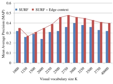
(26) HDR de Jean Martinet, Lille 1, 2016. .. . . . . . . . .. . . .. . . . .. Interest point Edge point Ed i t Gaussian cluster A vector drawn from an interest point to an edge one. Figure 2.1 – Extraction of the edge context descriptor in the 2D spatial space, after clustering the points in the 5-dimensional color-spatial feature space with a GMM. — an invariance to scale is achieved by normalizing the radial distance by a mean distance between the whole set of points inside the Gaussian; — an invariance to rotation is achieved by measuring all angles relative to the orientation angle of each interest point. After extracting the edge context descriptor, it is merged with SURF descriptor, and the final feature vector is composed of 88 dimensions: 64 from SURF + 24 from the edge context. The distribution of edge points enriches SURF descriptor with a local and discriminative information. Moreover, the distribution over relative positions yields a robust, compact, and highly discriminative descriptor. The set of features is then clustered with e.g. KMeans to form the visual vocabulary. Evaluation of the proposed descriptor We used the Caltech-101 dataset [FFFP07] to demonstrate the benefits of the proposed descriptor. Among the 8707 images of 101 classes in this dataset, we randomly selected 30 images from each class to build the visual vocabulary (i.e. 3030 images), and we randomly selected 10 other images from each class (1010 images) to build a test set. Query images are picked from this test set in the experiments. We used KMeans to construct the visual 11. © 2016 Tous droits réservés.. doc.univ-lille1.fr.

(27) HDR de Jean Martinet, Lille 1, 2016. vocabulary, with several values for K. For each value of K, we compare the accuracy of the proposed descriptor to the one of SURF taken alone.. Mean Average Precision (MAP). 0.6 SURF. SURF + Edge context. 0.5 0.4 0.3 0.2 0.1. 0. Visual vocabulary size K. Figure 2.2 – Comparison of the precision obtained with the proposed descriptor and with SURF taken alone, with different vocabulary sizes. Figure 2.2 shows the mean average precision (MAP) on all 101 object classes when the size of the visual vocabulary ranges from 1000 to 4000. We observe that we obtain the highest M AP value (0.483) with K = 2750 and with merging the local descriptors, which is over 30% of relative gain. More importantly, we see that for all different values of K, the proposed descriptor improves the accuracy over SURF. This descriptor is a part of the PhD of Ismail El Sayad, that include several contributions forming an image indexing and retrieval model. In this model, the descriptors are quantized to form a vocabulary tree, and visual words are filtered using a multi-layer pLSA [LRH09], and weighted as described in Section 2.3.1. In the part of his work, the contribution is essentially a new descriptor, that was published at CBMI’10 [ESMUD10a], and in more details in an MTAP journal paper [ESMUD12]. In the next two sections, we introduce alternative ways to build a visual vocabulary.. 2.1.2. Iterative vocabulary selection based on information gain. The motivation is here to propose a simpler, faster, and more robust alternative to the standard KMeans-based quantization step step used in bag-of-visual-words approaches. We designed a method for building a visual vocabulary, that consists in iteratively selecting visual words from a random set of features, using the tf-idf scheme and saliency maps. 12. © 2016 Tous droits réservés.. doc.univ-lille1.fr.

(28) HDR de Jean Martinet, Lille 1, 2016. Words selection and filtering Instead of using a clustering algorithm, the proposed method randomly selects descriptors among a large set of candidate visual words, and then iteratively filters out words in order to retain only the best words in the final vocabulary: 1. In the first step, a subset of candidate descriptors are randomly selected from a large and heterogeneous set (typically the whole set of descriptors from all images in a dataset) to form the initial vocabulary of visual words. All remaining descriptors are assigned to their closest visual word. 2. The second step iteratively identifies descriptors that have the highest information gain values in the candidate set: visual words with low information gain values are then discarded, and “orphan” descriptors (that were previously assigned to discarded words) are re-assigned to the closest remaining words. The initial vocabulary is purposely large, and the process iterates until the desired vocabulary size is reached. The information gain formulation IG for this work combines two sources: the tf-idf weighting scheme [vR79a] and Itti’s saliency maps [IKN98]: P nwD N SalwD log + (2.5) IGw = nD nw nwD where IGw is the information gain value of the visual word w, nwD is the frequency (i.e. the number of occurrences) of w in the dataset D, nD is the total number of descriptors in the dataset, N isP the number of images in the dataset, nw is the number of images containing the word w, and SalwD is the accumulated saliency score for all the keypoints assigned to word in w. Note that the standard tf for text is defined document-wise, and the formulation nnwD D Equation 2.5 is defined collection-wise. During each iteration, an amount of words (defined by a fixed ratio of the current vocabulary size) with lowest IGw value are discarded. This formulation means that the only words to be kept in the vocabulary have: — either a high tf-idf value, i.e. large number of occurrences in the collection, only in a limited number of images, — or a high saliency score, i.e. high saliency values for keypoints attached to the word, — or both a high tf-idf value and a high saliency score. Since the vocabulary is built from a random selection of words, it is natural to expect that several runs would produce different results. Although the experimental results proved little variations across different runs, we included in the method a stabilisation step to guarantee more stable results, that consists in combining several vocabularies. This idea is to generate k vocabularies as described above, and to combine them in a new set of words to be filtered again with the same iterative process. Experiments show that in addition to offering more stability, this process also further improves the results, since only the “best” words from k vocabularies remain in the final vocabulary. Note that the proposed method is feature-independant, and therefore it can be used with a wide variety of low-level features. 13. © 2016 Tous droits réservés.. doc.univ-lille1.fr.

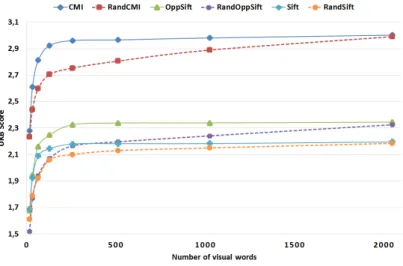
(29) HDR de Jean Martinet, Lille 1, 2016. Evaluation of the iterative process Two datasets were used in the experiments to validate our proposal: the University of Kentucky Benchmark (UKB) by Nistér and Stewénius [NS06] that contains 10,200 images, and the PASCAL Visual Object Classes challenge 2012 (VOC2012) [EVGW+ ] that contains 11,530 images. Since it is important in the proposed approach to pick random words from a large and heterogeneous feature set in order to give the selection process the best chance to end up with a high-quality vocabulary, another bigger dataset, MIRFLICKR-25000 dataset [HL08], was used to build the vocabulary. The main findings of the evaluation results are summarized below. — The first interesting result, as depicted in Figure 2.3, is that when using a mere random vocabulary (i.e. step 1 only, without the IG-based selection process), with a vocabulary size of 2000 words, the results are very similar to those obtained with a standard KMeans-based vocabulary of equal size on UKB images. Furthermore, this is true for several types of features we tried: Color Moments, Color Moments Invariants, SIFT, OpponentSIFT [vdSGS10], and SURF. Figure 2.3 shows the results for Color Moments Invariants (CMI), OpponentSIFT (OppSift), and SIFT. However, obtaining high results with a random vocabulary is mainly explained by the specificity of UKB retrieval dataset, where one query image is used to retrieve all 4 images of a given object under different viewpoints. Therefore, when the vocabulary size is large enough, the visual words selected with the random approach show sufficient diversity to be able to precisely select only the target object, without matching with other objects.. Figure 2.3 – KMeans-based vocabulary versus random selection of words. — Another noticeable result is that the IG-based selection process improves the performances, and best scores with UKB are reached with a very small vocabulary, e.g. 200-300 words, as shown in Figure 2.4; these scores are higher than the scores obtained 14. © 2016 Tous droits réservés.. doc.univ-lille1.fr.

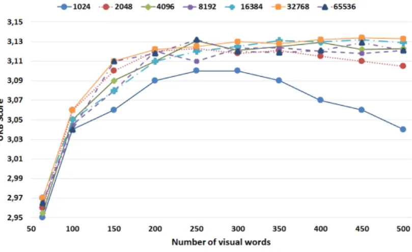
(30) HDR de Jean Martinet, Lille 1, 2016. with standard vocabularies of any size. This confirms that the iterative selection process helps selecting most useful visual words to represent the image content. With a vocabulary containing as little as 150 words, the iterative selection achieves higher scores than the KMeans-based vocabulary. Besides, despite the random nature of the method, we observed a high stability in the results after several runs.. Figure 2.4 – Iterative selection scores; the initial vocabulary size is 2048. — We found that it is important that the initial vocabulary size be large enough (e.g. over 2000 for UKB, that we see as a diversity threshold) to achieve high scores. However, above the diversity threshold, using larger initial vocabularies brings no improvement, as observed in Figure 2.5.. Figure 2.5 – Mean scores for several initial vocabulary sizes, from 1024 to 65536.. 15. © 2016 Tous droits réservés.. doc.univ-lille1.fr.

(31) HDR de Jean Martinet, Lille 1, 2016. — Finally, the combination of several vocabularies improves the selection of the “best” words, and increases the scores. Empirically, k = 3 proved to be optimal, and k ≥ 4 gives identical results and yet requires more processing. This improvement (about +7%) is observed with most low-level features on UKB, and the scores are higher than Fisher Vectors [PD07] or Vector of Locally Aggregated Descriptors (VLAD) [JDSP10]. Indeed, our highest score is 3.23 (with 256 visual words selected from 4096, using CMI and combining k = 3 vocabularies), while Jégou et al. [JDSP10] reported a score of 3.17 for VLAD, and 3.09 for Fisher Vectors, and 2.99 for a standard KMeans-based vocabulary (also with 256 visual words, using CMI). We also made experiments with Pascal VOC2012: the results are very similar to (however not higher than) those obtained with a standard vocabulary. Indeed, Pascal VOC2012 is a classification dataset with cluttered highly images, that is less suitable for retrieval. Nevertheless, the vocabulary construction process in the proposed approach is much lighter, and therefore the processing time is much shorter. In further research [LUG+ 16], we also compared 3 other information gain models in addition to tf-idf : tfc [SB88] (the term frequency component is a normalized version of tf-idf that includes the differences in documents’ length), Okapi bm25 of Roberstson et al. [RWH00] (the weight is based on a probabilistic framework) and an entropy formulation by Rojas López et al. [LJSP07] (the weight is based on the distribution of a term in a single document as well as in the whole dataset). We observed that except Okapi bm25, all information gain formulations give slightly better results than the standard vocabulary (about +2% for UKB and +4% for Holidays dataset [JDS08]). The results also confirm the low performance with Pascal VOC2012 for all information gain formulations. Besides, we showed that the iterative vocabulary selection can be successfully applied in the context of visual phrases, bringing about 3% increase in the UKB score. In addition, it should be highlighted that this method is robust since it yields high scores using a vocabulary that was built on a third party dataset, which is a good indication of versatile vocabulary. More details on the iterative vocabulary selection can be found in our ICMR’14 paper [UGL+ 14] and SIVP journal paper [LUG+ 16]. The next section introduces another alternative to standard vocabularies, in a mobile context.. 2.1.3. Split representation for mobile image search. This work was done in the context of image search on mobile devices in a scenario where image descriptors are extracted on the mobile device and transferred to a remote server for the retrieval task. The increasing popularity of mobile devices leads to a growing need to adapt image representation and retrieval methods to the constraints of such devices. Indeed, despite the huge technology advances, mobile devices are rather still limited in memory, speed, energy and bandwidth. To deal with these constraints, three scenarios for mobile image search were proposed by Girod et al. in [GCGR11]. 1. Server-side processing: The first one consists in transferring a compressed version of 16. © 2016 Tous droits réservés.. doc.univ-lille1.fr.

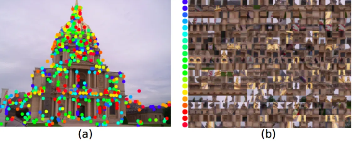
(32) HDR de Jean Martinet, Lille 1, 2016. the query image to a remote server that is in charge of extracting descriptors, retrieving the most similar images and returning results’ thumbnails to the mobile device. However, highly compressed images tend to contain visual artefacts that make difficult the detection of regions of interest. 2. Client-side processing: The second scenario consists in performing the whole retrieval task on the mobile device. It requires the whole database index to be stored on the device. Because the available memory is limited, the size of the database is restricted, even when using memory-efficient indexing methods. Moreover, the retrieval process is likely to require more computational power than the device can provide. 3. Hybrid method (shared processing): The last strategy consists in extracting the descriptors on the device, and to transfer them to the server for the retrieval task – possibly after a descriptor selection/compression step. For example, the Compressed Histogram of Gradients (CHoG) descriptor [CTC+ 09] was designed by Chandrasekhar et al. to follow this strategy. The approach proposed in this work also adopts the third strategy. We propose to limit the bandwidth use by reducing the amount of data required to describe images. During TWIRL project, José Mennesson, Pierre Tirilly and I proposed to leverage the repetitiveness (or burstiness [JDS09]) of visual elements in images, and build a lightweight representation of images. By taking advantage of this property, our approach represents groups of local descriptors as single representative descriptors, called elementary blocks, that are transmitted to the server. Assuming that images are composed of a set of elementary blocks, they can be represented using only a few well-chosen features extracted on the mobile device, and sent to the server for matching. The results are then sent back to the mobile device. This scenario is illustrated in Figure 2.6. Compared to the entire client-side processing and the entire server-side processing, this strategy is preferred to provide a good trade-off between hardware constraints (memory, speed, energy, and bandwidth) and retrieval effectiveness.. Figure 2.6 – Illustration of the mobile image search scenario.. 17. © 2016 Tous droits réservés.. doc.univ-lille1.fr.

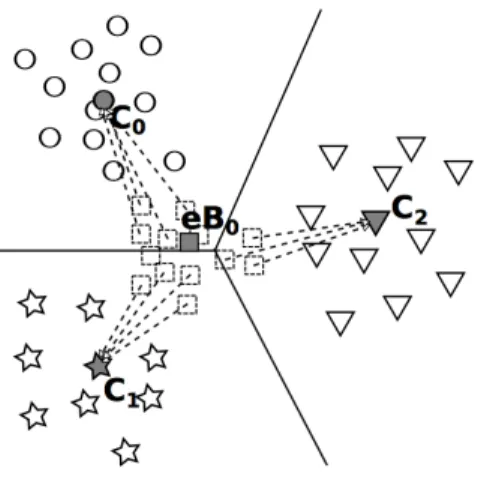
(33) HDR de Jean Martinet, Lille 1, 2016. Elementary blocks The key idea of the presented approach consists in having two different vocabularies: — one reference visual vocabulary (visual words), built only once, kept on the server side; — one local vocabulary (elementary blocks) that is built at query time on the device using a single image. From a given query image, local descriptors (e.g. SIFT) are extracted, and a quantization process determines the representative features eBi – with a record of the cluster sizes o(eBi ), that is to say the number of descriptors assigned to each cluster center eBi . Figure 2.7 shows an example of elementary blocks built using KMeans in a query image of Les Invalides from the Paris dataset [PCI+ 08] using SIFT descriptors and K = 20, i.e. 20 elementary blocks. Figure 2.7-(a) shows the keypoints locations; each keypoint color corresponds to a given block. Figure 2.7-(b) presents samples of visual elements belonging to each block. Some structures of the building emerge, such as pieces of roof, columns, balustrades, etc.. Figure 2.7 – Elementary blocks of Les Invalides. (a) SIFT keypoints are represented by colored dots; each color corresponds to a cluster. (b) Each row contains 25 sample patches from a given cluster. Best seen in color.. Elementary block assignment Once the elementary blocks are extracted from the query image, they are sent to the server. It is necessary to assign them to the reference visual words, in order to allow matching them with the dataset images. Of course, there is no guarantee for an eBi to perfectly correspond to a single visual word. A soft assignment function is used to assign an elementary block eBi to several reference words Cj according to their distances to the descriptor, using a weighting function. Euclidean distances between each eBi and all Cj (denoted D(eBi , Cj ) = ||eBi − Cj ||2 ) are computed, then normalized by rescaling them between 0 and 1 based on their minimum and maximum values. A radial weighting function w(eBi , Cj ) defines a weight, inspired from 18. © 2016 Tous droits réservés.. doc.univ-lille1.fr.

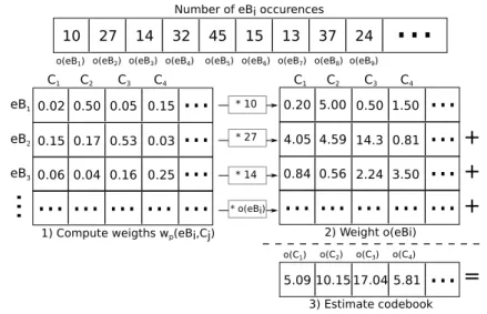
(34) HDR de Jean Martinet, Lille 1, 2016. Figure 2.8 – Assignment of elementary block eB0 to visual words C0 , C1 , and C2 . soft assignment methods [PCI+ 08, GCC+ 11], that is assigned to each (eBi , Cj ) pair: w(eBi , Cj ) = e−. D(eBi ,Cj ) 2σ 2. = e−κ×D(eBi ,Cj ). (2.6). where σ ∈ R+ is a free parameter controlling the slope of the exponential function and κ = 2σ1 2 . The parameter κ controls the softness of the assignment: high κ values will result in a steep slope for the radial function, and therefore a hard assignment to only close visual words; on the contrary, low κ values will give a moderate slope, so the assignment will be soft, and will consider visual words in a large neighbourhood. As illustrated in Figure 2.8, descriptors corresponding to eB0 can be assigned to C0 , C1 or C2 . In order to estimate the distribution of all o(eBi ) descriptors over the visual vocabulary, these weights are divided by the sum of these quantities over the vocabulary: w(eBi , Cj ) wn (eBi , Cj ) = PNC j=0 w(eBi , Cj ). (2.7). where wn is the normalized weighting function and NC is the size of the visual vocabulary. The final number of occurrences o(Cj ) of the visual word Cj is estimated with: o(Cj ) =. NeB X. wn (eBi , Cj ) × o(eBi ). (2.8). i=0. where NeB is the total number of elementary blocks. This assignment process is illustrated Figure 2.9. Evaluation of the split representation We conducted experiments varying the vocabulary size NC and the number of elementary blocks NeB , using three datasets: Paris [PCI+ 08], Oxford [PCI+ 07], and Holidays [JDS08]. 19. © 2016 Tous droits réservés.. doc.univ-lille1.fr.

(35) HDR de Jean Martinet, Lille 1, 2016. Number of eBi occurences. 10. 27. 14. 32. o(eB1) o(eB2) o(eB3) o(eB4). C1. C2. C3. 45. 15. 37. 24. .... o(eB5) o(eB6) o(eB7) o(eB8) o(eB9). C4. C1. C2. C3. C4. ... 0.20 5.00 0.50 1.50 4.05 4.59 14.3 0.81 0.15 0.17 0.53 0.03 ... 0.84 0.56 2.24 3.50 0.06 0.04 0.16 0.25 ... ... ... ... ... ... ... ... ... ... .... eB1 0.02 0.50 0.05 0.15. * 10. eB2. * 27. eB3. 13. * 14. .... * o(eBi). ... ... + ... + ... +. 2) Weight o(eBi). 1) Compute weigths wp(eBi,Cj) o(C1). o(C2). o(C3). o(C4). 5.09 10.15 17.04 5.81. ... =. 3) Estimate codebook. Figure 2.9 – Assignment of eBi to Cj to estimate the associated visual word histogram. We used a vocabulary size NC ∈ [5.000, 50.000], and the number of elementary blocks NeB was set to a fixed ratio of the number of descriptors ND extracted from the query image (with typically ND < 2.000): NeB = α × ND , with α ∈]0, 1]. Since the number of keypoints per image is limited, the running time of KMeans for block computation is acceptable (< 1 second). Table 2.1 reports running times of Kmeans for various values of K (i.e. NeB ) and various numbers of descriptors (ND ), with a desktop computer 1 . ND α = 0.3 α = 0.5 α = 0.7. 500 1,000 2,000 0.05 s. 0.20 s. 0.58 s. 0.07 s. 0.21 s. 0.77 s. 0.08 s. 0.26 s. 0.87 s.. Table 2.1 – Running time (in seconds) of KMeans with NeB = α × ND . The main experimental results are summarized in Table 2.2. They show that with α = 0, 3 (i.e. when using only one third of the descriptors extracted from the query image), we can achieve results similar to the standard vocabulary approach. For Paris and Oxford datasets, the mean Average Precision (mAP ) values are even higher with the proposed approach than with the standard vocabulary in most settings. For Holidays dataset, the proposed approach did not achieve the same results as the standard approach. The main reason is that in this dataset, contrary to the two other datasets, query images require various query-specific settings for NeB (number of elementary blocks) to reach similar results. Therefore, a query-specific setting of α would be more suited than using a fixed value for all queries. 1. We have not tried yet to run the system on a mobile device. We used a desktop computer with Intel core 2 CPU 2.66GHz×2, 2GB RAM.. 20. © 2016 Tous droits réservés.. doc.univ-lille1.fr.

(36) HDR de Jean Martinet, Lille 1, 2016. NC Database. Paris. 5,000 Oxford. Holidays. Paris. 10,000 Oxford. Holidays. Paris. 50,000 Oxford. Holidays. Baseline Random 30% Random 50% Random 70% Ours (α = 0.3) Ours (α = 0.5) Ours (α = 0.7). 36.83 33.74 35.60 36.59 37.20 37.25 37.16. 33.48 29.71 31.78 32.21 31.25 33.69 33.97. 48.41 42.78 44.26 46.93 43.16 46.12 46.95. 36.18 34.98 36.31 35.93 37.88 37.52 36.79. 33.33 32.43 32.79 33.12 34.49 33.98 33.78. 44.85 43.64 44.25 44.50 43.93 44.76 44.30. 50.40 44.17 47.91 49.16 46.86 49.82 50.66. 42.89 36.39 40.14 40.42 36.75 40.52 42.90. 60.10 53.34 57.28 59.40 49.99 55.83 58.99. Table 2.2 – mAP (in %) on Paris, Oxford and Holidays datasets for a standard approach (baseline), a vocabulary with randomly sampled descriptors, and our method using different values of NeB , NC . Results above the baseline are shown in bold. We also found in the experiments that the optimal value of κ depends on the vocabulary size: smaller κ values are needed with larger vocabularies. Indeed, a high number of visual words implies a sparse space. This means that we get a larger number of histogram bins, and consequently a reduced chance to find matching eBi in similar images. Therefore, it is necessary to distribute the query image descriptors over more reference words in order to maximize the chances of matching. In this case, such a soft assignment brings a solution to a sparse feature space. Besides, for Paris and Oxford datasets, higher values of NC will require higher values of α to outperform the standard approach. In other words, with a large vocabulary, a large number of elementary blocks is needed. Once again, when the space becomes sparse, a higher number of descriptors will increase the chance of matching for similar images. Finally, Table 2.2 also shows the results of a random sampling among query image descriptors. Random sampling generally gives lower results, justifying the need to carefully select elementary blocks e.g. with the proposed approach. It is intersting to notice that here, even though the matching process is different, the behaviour with the random sampling is similar to this of the approach presented in the previous Section 2.1.2 (see in particular Figure 2.3): in both cases, the random sampling of descriptors yields results slightly lower than the baseline, and such results increase with the number of sampled descriptors until the baseline level reached. In summary, the presented method shows that using only one third of the query image descriptors, we can achieve results comparable to the bag-of-visual-words approach for Paris and Oxford datasets. Coming back to the objective of the method, it is an aceptable trade-off between hardware constraints and retrieval effectiveness. For example, with ND = 1000 and α = 0.3, the average clustering time in our experiments was 0.20 sec. In this setting, the size of data to be transmitted to the server is 1000 × 512 B = 500 KB (512 bytes is the size of 1 SIFT descriptor) for the standard approach, and 500 KB × 0.3 = 150 KB for the proposed approach. For a comparison, the first strategy described earlier in this section would require to send the entire image (say 1 MB) to the server. More details on these experiments and results can be found in our ICIP’14 paper [MTM14].. 21. © 2016 Tous droits réservés.. doc.univ-lille1.fr.

(37) HDR de Jean Martinet, Lille 1, 2016. 2.1.4. Textual vs. visual words. As a last part of Section 2.1 related to visual vocabularies, we discuss here the very notion of visual words, and the application of text processing techniques (e.g. word filtering, weighting, etc.) to such words. Most of existing approaches for visual words are inspired from the workwork in text indexing, based on the implicit assumption that visual words can be handled the same way as text words. However, to the best of our knowledge, no work ever casted doubt on this assumption for visual words. Zipf ’s law and Luhn’s model A central aspect of text IR approaches is that they rely on important characteristics of the words distribution in a natural language. Zipf’s law links word frequencies in a language to their ranks, when they are taken in decreasing frequency order [Zip32]. This law stipulates that words occurrences follow a distribution model given by: Pn =. 1 na. (2.9). where Pn is the occurrence probability of the word at rank n, and a is a value close to 1. For instance, in large text collections in english language, the term “the” is generally the most frequent, representing about 7% of the total word count. The second most frequent is “of ”, with 3,5% of the total, etc. As an illustration, Figure 2.10-(a) shows the word distribution from Wikipedia entries in November 2006 1 in a bi-logarithmic plot, which reveals the logarithmic distribution. This logarithmic distribution, interpreted with Shannon’s information theory [Sha48], laid down the theoretical foundations of word filtering and weighting schemes. In particular, early selection techniques for significant terms were mainly grounded on hypotheses from Luhn’s model [Luh58], and this model originates from Zipf’s law. This model indicates a relation between the rank of a word and its discriminative power (or resolving power), that is to say its capacity of identifying relevant documents (notion of recall) combined with its capacity of distinguishing non-relevant documents (notion of precision). This relation is illustrated Figure 2.10-(b): less discriminative words are those with a low rank (very frequent), and also those with a high rank (very rare). The most discriminative words are those located in-between, and therefore these terms should be selected to create the indexing vocabulary. Relations between words distribution and search performance Interestingly, we found in our experiments that the visual words distribution highly depends on the clustering method used to build the vocabulary, and less on the descriptor. We used two image datasets: Caltech-101 [FFFP07] and Pascal VOC2012 [EVGW+ ]. In this work, 1. Source : Wikipedia, URL : http://en.wikipedia.org/wiki/File:Wikipedia-n-zipf.png.. 22. © 2016 Tous droits réservés.. doc.univ-lille1.fr.