Evaluation of the Phase Distribution in an Interferogram by the Wavelet Method

(1)

Ministry of Higher Education and Scientific Research Ferhat Abbas University – Setif

MEMOIRE

Defended at the Faculty of Engineering Science Department of Optics and Precision Mechanics

In view to obtain the Diploma of

MAGISTERE

In Optics and Precision Mechanics Option: Applied Optics

By Regoui Cherif

THEME

Evaluation of the Phase Distribution in an Interferogram by the Wavelet Method

Defended on 11 / 06 / 2007 Before the committee composed of :

Dr Demagh N. M.C at Setif University President

Dr Bouamama L. M.C at Setif University Supervisor

Dr Manallah Ah. C.C at Setif University Examiner

Dr Belkhir AH. C.C at Setif University Examiner

(2)

Acknowledgements

I wish to show my gratitude to Dr Larbi Bouamama for proposing this very interesting subject, for his advices and his utter availability throughout this work

I would like to thank Dr Nacereddine Demagh for having accepted to criticize this work and to preside the committee.

My thanks go to Dr Ahmed Manallah for his kindness and the discussions we had about various subjects in general and optics in particular, and for having agreed to examine this work.

My gratitude go to Dr Abdel Hak Belkhir for the exchanging of views and his curiosity about optics and to have approved to give his evaluation about this task.

I thank also Dr Messaoud Djabi for his interest in the subject, for his gentleness and benevolence to judge this undertaking.

(3)

(4)

Accurate measurements are very important in the development of science and engineering. Optical measuring methods have proved to be very useful especially interferometry [1,2,3,4]. The resulting fringe pattern, called interferogram, is closely related to phenomenon under inspection and useful information can be retrieved. The analysis of the interferogram is the key to obtaining the needed information. Several techniques of analysis have been devised, some of the more known are the phase-shifting and the Fourier transform techniques [5,6,7]. These techniques give very good results but they have some serious drawbacks: they lack the time-frequency localization and they need at least three interferograms to retrieve the phase information.

To circumvent these inconveniences, several techniques have been proposed. One of the most promising is the use of the continuous wavelet transform [8,9,10]. It is still a matter of intensive research and progress is made continuously.

Our work focuses on the use of the continuous wavelet transform to extract the phase distribution from simulated interferograms.

In the first chapter, devoted to the basic laws of optics, we discuss the nature of light and the interference and diffraction phenomena.

In chapter 2 we delve into the interferometers and the ways to obtain the fringe pattern. We discuss holography as a special experimental technique that is based on both interference and diffraction.

The techniques of fringe analysis are reviewed in chapter 3. An emphasis is done on the phase shifting technique and the Fourier transform and its main drawbacks.

The fourth chapter which represents the main part of our work deals with the definition, properties and the use of the continuous wavelet transform to extract the phase distribution from simulated interferograms. It begins by reviewing the time-frequency concept, the Heisenberg boxes, the Fourier and Gabor transforms, then we

(8)

focus ourselves on the wavelet transform technique where we present the mathematical justification of its adequacy to fringe analysis, then the procedure of extraction of the phase from the simulated interferogram. In order to check our results, we use the phase shifting method.

(9)

Chapter 1

The nature of light

1.1 Introduction

Light is all known but mysterious. Its very nature has been the subject of long discussion between scientists for long periods of time. Sometimes it behaves like a wave, other times like a particle. It can be described as rays. It is accepted that it is all of this and depends only on the way we measure it.

1.2 The particle nature of light

The particle nature of light was established by the photoelectric effect explained by Einstein in one of his famous papers of 1905 [11], the annus mirabilis (miraculous year) where he also laid the principles of special relativity [12]. The light is considered to be a grain of energy characterized by a frequency. The relationship between the frequency  of the photon and its energy W is [13]:

W h, (1) where h is Planck’s constant with

_h__{6.63 10}_ 34_Js_{. (2)}

1.3 The wave nature of light

The wave nature of light is revealed by phenomena like interference and diffraction. In the middle of the 19th century J.C Maxwell gave a framework that could encompass its electromagnetic wave nature.

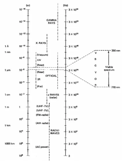
1.3.1 The electromagnetic spectrum

Electromagnetic waves encompass a large spectrum of radiation. They extend from the cosmic rays (the more energetic) to the radio waves (the less energetic) including the

(10)

ultra-violet, the x and gamma rays, the infra-red and the radar and TV rays andvisible light.

Figure 1.1 shows the electromagnetic spectrum with the place that visible light occupies in it.

Figure 1.1 The electromagnetic spectrum.

1.3.1 Maxwell’s equations

Maxwell could summarize electromagnetic phenomena and light in a set of elegant and compact equations that are in differential form [14]:

(11)

divD (3a) divB 0 (3b) curl t     B E (3c) curl t     D H j (3d) These equations are supplemented by three material equations:

DE , BH , jE (4)

where E : is the electric field vector,

B : is the magnetic induction vector, H : is the magnetic field vector, D : is the displacement vector,

 : is the electric charge density,  : is the electric permittivity constant,  : is the magnetic permeability constant,  : is the specific electric conductivity.

Light can be considered consisting of an electric vector field E and a magnetic vector H (figure 2.2) propagating perpendicular to each other and to k , the direction of propagation (in an isotropic medium).

Figure 1.2 An electromagnetic wave.

By combining these equations one can obtain for the electric field vector, the wave equation in a homogeneous, isotropic medium:

(12)

2 2 2 1 0 v t      E E (5) where v is the velocity of light in the medium.

v is related to the velocity of light in free space c by: v = c

n, (6) with _c_{ }_{3 10 ms}8 1_{. (7)} Here n is the refractive index of the medium.

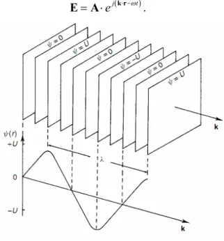
A solution of the wave equation is the plane wave (see figure 1.3) given in complex form by:

j t

e     k r

E A . (8)

Figure 1.3 A plane wave.

where:

k r t: is the phase of the wave. k : is the wave vector, with k 2



 , being the wavelength of the wave.

A : is the amplitude.

: is the angular frequency. It is related to the frequency by:

(13)

Knowing that  v 

 , the relation between the wavenumber and the angular frequency is

kv. (10) A plane wave is also called a harmonic wave and can be represented by:

E A cos



k r t



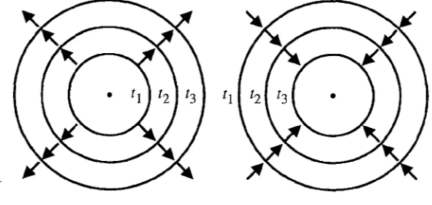
. (11) In the remainder we will use the symbol U (or U in scalar form) to denote either the electric field E or the magnetic field H .

Another solution to the wave equation is the spherical wave: _{U r}( ) A_e j kr t

r



 

 , (12) where r is the distance from the source. Figure 1.4 shows converging and diverging waves.

Figure 1.4 Converging (right) and diverging (left) spherical waves.

1.3.2 Phase velocity and group velocity

1.3.2.1 Phase velocity

Let’s assume that a monochromatic light propagates in the z direction. The equation of the electromagnetic perturbation will be [15,16,17]:

(14)

from which:

vp

k 

 . (14)

is the phase velocity.

1.3.2.2 Group velocity

Now, let’s assume that we have the superposition of two waves with slightly different values of k and. The first one is characterized by a wavenumber k and an angular velocity, the second with corresponding k  and k   respectively. The total  electromagnetic perturbation will be

_U __ej kz t



1__e  j kz t



_{, (15)}

The total electric field will be

( )_cos( ₎ 2

j kz t k z t

U_e       _{. (16)} The cosine factor is an envelope function that modulates the traveling waves (figure 2.5). The envelope travels at the velocity of:

vg k     (17) called the group velocity. In the case where   and  0   the group velocity will k 0 be the derivative

v_g d dk



 . (18)

Phase and group velocities are related by

v v vp g p d k dk   . (19) 1.3.4 Interference of light

The Maxwell’s equations as well as the wave equation are linear. This leads to the possibility of application of the superposition principle.

(15)

1.3.4.1 Principle of superposition

It states that if two waves whose amplitudesU and ₁ U exist in the same portion of space ₂ it results a wave whose amplitude U is simply:

U U ₁U₂. (23)

1.3.4.2 The interference equation

When two monochromatic waves are superposed, the result is a monochromatic wave of the same frequency [22,23,24,25].

We will consider the addition of waves of the same frequency, the consequence of which is the observation of bright and dark bands of light called fringes. In every day life these fringes are commonly observed for example in soap bubbles or on oil films in wet roadways.

Obtaining the interfering waves is generally done by dividing one beam of light into two or more beams. The way of dividing the light beam provides a basis for classifying the arrangement used to produce interference.

In one, the beam is divided by passage through apertures placed side by side. This method, called wavefront division, is only useful with sufficiently small pieces.

In the other, the beam is divided at one or more partially reflecting surfaces at each of which part of the light is reflected and part transmitted. This method is called amplitude division. It can be used with extended sources and the effects may be of greater intensity than with wavefront division.

It is convenient to consider separately the effects which result from the superposition of two beams (two-beam interference) from those which result from the superposition of more than two waves (multiple-beam interference).

Let us consider two coherent monochromatic waves 1

1 i U Ae and 2 2 i U Ae . The intensity of the resulting wave will be:







*

1 2 1 2

(16)

* * * *

1 1 2 2 1 2 1 2

I U U U U U U U U (24) And finally after replacing each quantity by its expression we get:

I  I₁ I₂ 2 I I_{1 2}cos (25) where *

1 1 1

I A A : is the intensity of the first wave. *

2 2 2

I A A : is the intensity of the second wave.

   ₂ : is the phase difference between the two waves.₁

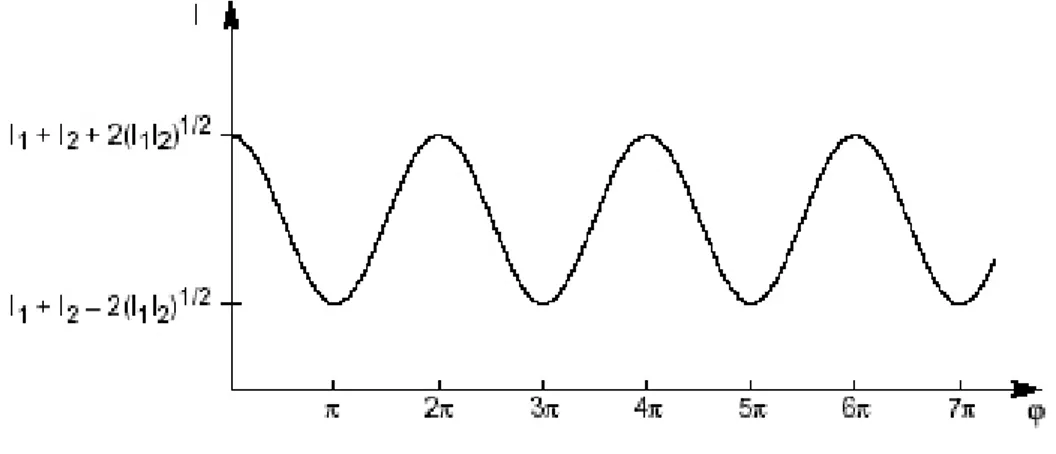
This is the fundamental equation of the interference phenomena. It shows that the resulting intensity is not simply the sum of the interfering intensities but a third term

1 2

2 I I cos, intervenes. It is called the interference term. The intensity variation with respect to the phase is shown in figure 1.6.

Figure 1.6 Intensity distribution with respect to the phase.

Some particular cases are worth mentioning:

- If the phase difference is an integral number of 2 rd then the intensity is at its maximum and we have a bright fringe: 2m , m  0, 1, 2,...

(17)

- If the phase difference is an odd integral number of rd 2 

then the intensity is at its

minimum and we have a dark fringe: 2 1 2 m

   , m  0, 1, 2,...

I_min   I₁ I₂ 2 I I_{1 2} 



I₁ I₂



2 (27) - If the interfering waves have the same intensityI₁I₂  , the visibility of the fringes I₀ will get its maximum value and the intensity will be

2 0 4 cos 2 I  I  _{ }  . (28)

In this case the intensity of the resulting wave varies from I to ₀ 4I (and not ₀ fromI to₀ 2I ) as shown in figure 2.7:₀

Figure 1.7 Intensity distribution in the case the interfering waves are amplitude equal.

1.3.5 Diffraction of light

It has been defined by Sommerfeld as any deviation in the path of light rays that cannot be explained as a reflection or refraction.

However, there is no substantive difference between diffraction and interference. The separation between the two subjects is historical in origin and is retained for pedagogical reasons[26]. Interference may be associated with the intentional formation of two or more light waves. Diffraction may be associated with the obstruction of a single wave, by a

(18)

transparent or an opaque obstacle, resulting in the obstruction casting shadows (or forming light beams) that differ from the size predicted by geometrical optics. This distinction between interference and diffraction is, however, arbitrary (figure 1.7).

Figure 1.7 Simlarity between diffraction and interference.

1.3.5.1 The Huygens-Fresnel principle

The application of the rigorous theory is very difficult and for most problems an approximate scalar theory is used. The approximate scalar theory is based on Huygens’ Principle that states:

Each point on a wavefront can be treated as a source of a spherical wavelet called a secondary wavelet or Huygens' wavelet. The envelope of these wavelets, at some later time, is constructed by finding the tangent to the wavelets. The envelope is assumed to be the new position of the wavefront.

(19)

Figure 1.8 Huygens-Fresnel principle.

Diffraction effects are a consequence of the wave nature of light. Even if the obstacle is not opaque and presents variations in amplitude or phase of the wave front, diffraction is present. Imperfections in the glass produce diffraction patterns too when transmitting light.

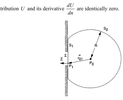
1.3.5.2 The Fresnel-Kirchhoff diffraction formula

In the study of diffraction (figure 1.9), Kirchhoff made some assumptions [27,28]: - Across the surface  , the field distribution U and its derivative dU

dn are exactly the same as they would be in the absence of the screen.

- Over the portion of S that lies in the geometrical shadow of the screen, the field ₁

distribution U and its derivative dU

dn are identically zero.

Figure 1.9 Fresnel-Kirchhoff diffraction by a planar aperture.

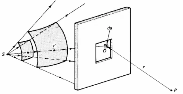
When the distance from the aperture to the observation point is usually many optical wavelengths the Fresnel-Kirchhoff diffraction formula can be derived:

(20)

 

₀   cos ,

 

cos ,

 

2 jk r s A e U P dS j rs    

_

n r n s (29)

1.3.5.3 Fresnel diffraction

In the study of diffraction approximations are made to simplify the task. If either or both aperture or observing screen are close enough so that the curvature of the wavefront has to be taken into account (figure 1.9), we are in the case of Fresnel diffraction or near-field diffraction.

Figure 1.10 Layout of Fresnel diffraction.

The approximation is based on the binomial expansion of 1 where   is very small towards unity. We have:

2 4 1 1 2 8          . (30) The distance r from the aperture to the observation screen can be written:



 





 





 



2 2 2 2 2 2 2 2 1 1 2 2 r x y z x y z z x y z z z                  _ _           (31)

(21)

 





    2 2 2 2 2 2 2 , , k k jkz _j _x _y _j _j _x _y z z z e U x y e U e e d d j z                     _ _  

 

. (32)

This is known as the Fresnel diffraction integral.

Aside from the multiplicative constants, we that it is the Fourier transform of the product of the complex field just to the right of the aperture and a quadratic phase exponential.

1.3.5.3 Fraunhofer diffraction

There exists a more stringent approximation that makes the calculations much easier. It is the Fraunhofer approximation, or the far field diffraction. If in addition to the Fresnel approximation, we add that





2 2 max 2 k z   , (33) then the quadratic phase factor under the integral sign is approximately unity over the entire aperture, and the observed field strength can be found by

 





  2 2 2 2 , , k jkz _j _x _y _j _x _y z z e U x y e U e d d j z               

 

. (34)

This is simply (aside from the multiplicative term before the integral sign) the Fourier transform of the aperture distribution.

(22)

Chapter 2

Interferometry

2.1 Introduction

After having viewed the characteristics of light, we see now how its wave nature is used in some setups, called interferometers. The devices studied here, are based on the interference phenomenon.

Interferometric devices can be considered in two categories: those based on optical interferometry and those based on the more recent holographic interferometry that appeared after the invention of the laser and the development of holography.

2.2 Optical interferometry

Interferometric measurements require an optical arrangement in which two or more beams, derived from the same source but traveling along separate paths, are made to interfere. Interferometers can be classified as two-beam interferometers or multiple–beam interferometers according to the number of interfering beams[29].

2.2.1 Two beam interferometers

2.2.1.1 Michelson interferometer

This instrument is shown schematically in figure 2.1. A partially silvered mirror allows a single beam of light to fall on two mirrors, M1 and M2. The mirrors are adjusted to recombine the resulting two beams in a line with the observer's eye.

(23)

Figure 2.1 The Michelson interferometer.

Looking into the beam splitter, we seem to see both M1 and M2 in approximately the locations of figure 2.2 .

The mirrors are apparently separated by

2 1

d l  (1)l and interference maxima occur when

2 cosd  m (2)

(24)

Because two beams are involved, the interference pattern is described by _{cos fringes.}2 The interference pattern appears the same as that brought about by two nearly parallel surfaces with low reflectance. In the interferometer, however, the separation and orientation of the mirrors are adjustable. If the mirrors are tilted slightly with respect to one another, the fringes are nearly straight and parallel to the line of intersection of the mirror planes and are called fringes of equal thickness. If the mirrors are parallel, but separated somewhat, symmetry dictates circular fringes whose maxima occur at certain angles  that depend on the value of d; these are called fringes of equal inclination. Michelson used the interferometer to measure the wavelength of light in terms of a material standard of length, which ultimately became the standard meter.

2.2.1.2 Mach-Zehnder interferometer

This instrument is shown in figure 2.3. Although not truly a relative of the Michelson interferometer, it is nevertheless a two-beam interferometer that works by division of amplitude. Because it is a single-pass interferometer, the Mach-Zehnder has only half the sensitivity of the Michelson or Twyman-Green interferometers. Like the latter, it may be used for testing optics for flatness, thickness variation and so on; it has also been used for measuring the index of refraction of gases.

(25)

The interferometer consists of two mirrors and two beam splitters. The first beam splitter divides the beam into two parts, whereas the second combines the parts after reflection from the two mirrors. In the figure, a test piece is located in the lower arm. The upper arm contains a compensator that is needed when the source has limited temporal coherence; the compensator has roughly the same optical thickness as the specimen and ensures that the two arms have nearly equal optical path length. If the source is a laser, the compensator is superfluous.

2.2.1.3 Twyman-Green interferometer

This instrument is closely related to the Michelson interferometer and resembles a Michelson interferometer illuminated with collimated light (figure 2.4). It is used to test flat optical windows and other optics whose transmission (as opposed to reflection) is important.

Figure 2.4 Twyman-Green interferometer

The Twyman-Green interferometer is set up with collimated light; the mirrors are adjusted sufficiently parallel that a single fringe covers the entire field. A test piece, say an optical flat, is inserted in one arm. Any fringes that appear as a result of the flat's

(26)

presence represent optical-path variations within the flat. For example, if the flat is slightly thicker on one side than on the other, it is said to have a wedge. Looking through the flat makes the mirror appear slightly tilted and results in nearly straight fringes. Similarly, if the surfaces are not flat, but slightly spherical, the fringes will appear circular.

The Twyman-Green interferometer is also used for testing lenses. One mirror is replaced by a small, reflecting sphere, and the lens is positioned so that the center of the sphere coincides with the focal point of the lens. Plane waves thus return through the lens if the lens is of high quality. Aberrations or other defects in the lens cause the returning wavefronts to deviate from planes and result in a fringe pattern that can be used to evaluate the performance of the lens.

2.2.1.4 The Sagnac interferometer

In the Sagnac interferometer, as shown in figure 2.5, the two beams traverse the same closed path in opposite directions. Because of this, the interferometer is extremely stable and easy to align, even with an extended broadband light source.

(27)

Modified versions of the Sagnac interferometer have been used for rotation sensing. When the interferometer is rotated with an angular velocity  about an axis making an angle  with the normal to the plane of the interferometer, a phase shift  is introduced between the beams given by the relation

8 Acos c      (3)

where A is the area enclosed by the light path,  is the wavelength , and c is the speed of light .

2.2.1.5 The Fizeau Interferometer

In the Fizeau interferometer, as shown in figure 2.6, interference fringes of equal thickness are formed between two flat surfaces separated by an air gap and illuminated with a collimated beam. If one of the surfaces is a standard reference flat surface, the fringe pattern is a contour map of the errors of the test surface. Modified forms of the Fizeau interferometer are also used to test convex and concave surfaces by using a converging or diverging beam.

(28)

2.2.1.6 Polarization interferometers

Polarization interferometers have found their most extensive application in interference microscopy. The Nomarski interferometer, shown schematically in figure 2.7, uses two

Figure 2.7 The Nomarski interferometer.

Wollaston (polarizing) prisms to split and recombine the beams. If the separation of the beams in the object plane (the lateral shear) is small compared to the dimensions of the

2.2.1.7 Wavefront division interferometry

Young’s double slit is the first interferometric setup. It is shown in figure 2.8.

(29)

Two of the most famous wavefront division interferometers, Fresnel’s biprism and Lloyd’ s mirror are shown below in figures 2.9 and 2.10.

Figure 2.9 Fresnel’s biprism.

Figure 2.10 Lloyd’s mirror.

2.2.2 Multiple-wave interferometers

2.2.2.1 Fabry-Perot interferometer

The Fabry-Perot interferometer consists of two parallel surfaces with highly reflecting, semitransparent coatings (figure 2.11).

(30)

The Fabry-Perot interferometer consists of two highly reflecting mirrors maintained parallel to great precision. As we found before, a given wavelength is transmitted completely only when

m2 cost  (4)

Like a diffraction grating, a Fabry-Perot interferometer is thus able to distinguish between wavelengths. It can be used in one of two ways. If the value of d is fixed and the interferometer illuminated with a slightly divergent beam, a given wavelength will be transmitted at several particular values of  only. Another wavelength will be transmitted at other values of ; the difference between the two is easily calculated. Often, only the difference is of interest; otherwise, a known wavelength must be introduced to calibrate the interferometer.

A Fabry-Perot interferometer is also used in a mode in which t is varied, generally with 0

  . Scanning may be accomplished by placing the entire instrument in a vacuum chamber and slowly lowering the pressure. This changes the optical thickness nt of the air between the plates, because n varies very nearly in proportion to the density or pressure of the air. Data collection by this method is relatively slow. Most modern instruments have one mirror fixed to a piezoelectric crystal (whose thickness varies with applied voltage) or to a magnetic drive similar to a loudspeaker. This mirror is rapidly driven back and forth through a few wavelengths, and the transmitted intensity is displayed on an oscilloscope or digitized by a computer.

2.2.2.2 Three-beam Interferometers

Zernike’s three-beam interferometer, shown schematically in figure 2.12, uses three beams produced by division of a wavefront at a screen containing three parallel, equidistant slits. In this arrangement, the optical paths of all three beams are equal at a point in the back focal plane of the lensL . The two outer slits provide the reference ₂ beams, while the beam from the middle slit, which is twice as broad, is used for measurements.

(31)

Figure 2.12 Zernike’s three-beam interferometer.

The intensity at any point in the interference pattern is then given by the relation

I I₀



3 2cos 2 4cos cos 



(5) where is the phase difference between the two outer beams, and is the phase difference between the middle beam and the two outer beams at the center of the field.

2.3 Holographic interferometry

With the method of holography now at hand, we are able to realize a type of experiment by storing the wavefront scattered from an object in a hologram. We then can recreate this wavefront by hologram reconstruction, where and when we choose. For instance, we can let it interfere with the wave scattered from the object in a deformed state. This technique belongs to the field of holographic interferometry [30,31,32].

In the case of static deformations, the methods can be grouped into two procedures, double-exposure and real-time interferometry.

2.3.1 Double-exposure interferometry

In this method, two exposures of the object are made on the same hologram. This might be recordings before and after the object has been subject to load by, for instance, external forces or two other object states that are to be compared. By reconstructing the hologram, the two waves scattered from the object in its two states will be reconstructed

(32)

simultaneously and interfere. This double-exposed hologram can be stored and later reconstructed for analysis of the registered deformation at the time appropriate for the investigator. If a lot of different states of the object (e.g. different load levels) are to be investigated, many holograms have to be recorded, which makes the method time-consuming and elaborate.

2.3.2 Real-time interferometry

In this method, a single recording of the object in its reference state is made. Then the hologram is processed and replaced in the same position as in the recording. By looking through the hologram we are now able to observe the interference between the reconstructed object wave and the wave from the real object in its original position. Thus we are able to follow the deformation as it develops in real time by observing the changes in the interference pattern. These changes might be recorded on film for later playback and analysis. A disadvantage of the method is that the hologram must be replaced in its original position with very high accuracy. This can be overcome by developing the hologram in situ in a transparent cuvette or using a thermoplastic film. Also the contrast of the interference fringes is not as good as in the double-exposure method.

(33)

Chapter 3

Methods of fringe analysis

3.1 Introduction

The outcome of interferometry techniques is a set of fringes called interferogram. With development and decreasing cost of digital image processing equipment, a growth has come in the digital fringe pattern measurement techniques [33,34,35,36]. Its benefits are essentially:

- better accuracy, - increasing speed, - automated process.

Automatic fringe pattern analysis is now used, with appropriate interferometers, in areas such as optical testing, flow visualization, non-destructive testing, industrial inspection and medical imaging. There are image processing techniques which can be used as the building blocks for an automatic fringe analysis system.

The quantitative evaluation in interferometric metrology consists of two steps:

the first and crucial one is the determination of the interference phase distribution from the recorded and stored fringe pattern,

the second is the combination of the phase data with data describing the optical arrangement to yield the displacement vector field, the optical path difference, the surface heights or the refractive index field, etc…

3.2 Intensity-based analysis methods

The fringe counting methods search for local brightness extrema, that correspond to phase values being integer multiples of. This method gives non uniform sampling, sub-wavelength variations may be overseen.

Phase stepping point-wisely evaluates with high accuracy but requires a set of three or more interferograms, reconstructed with a constant mutual phase shift.

(34)

They are the oldest in digital analysis of interferograms. They are used when:

- sometimes they are the only viable when interferograms are retrieved from photographic records;

- interferograms where it is impossible or impractical to use phase-based techniques; - quantitative results are not needed.

For these techniques, it is very important to reduce noise including speckle noise. Among these techniques are the prior knowledge and fringe tracking and thinning.

3.3 Phase-measurement interferometry

With a digital image-processing system, it is possible to store an image of the interferogram in the computer memory and then perform manipulations on the individual pixels.

The general expression of the intensity distribution of an interferogram is:

I   I₁ I₂ 2 I I_{1 2}  cos( ) . (1a)

We would expect to retrieve the phase simply by computing:

1 1 2 1 2 ( ) cos 2         _ _   I I I I I . (1b) This supposes that we know the values ofI ,I ,1 I and 2  for each pixel. And thereby, by knowing the geometrical and optical arrangement of the interferometer we could evaluate the parameter under study for each pixel.

This assumption is unrealistic for most cases. Furthermore, even if we had that ideal interferogram, a complex optical system will induce uncontrollable noise.

(35)

3.3.1 Principles of temporal phase-measurement interferometry The general expression of the intensity of a recorded interferogram is:

I x y( , )a x y( , )b x y( , ) cos ( , )



 x y (2a)



( , ) ( , ) 1 ( , )cos ( , )





( , )     _  _   b x y I x y a x y x y a x y (2b) I x y( , )a x y( , ) 1



V x y( , ) cos ( , )



 x y





(2c)

I , a , b and  are functions of the pixel coordinates. ( , )

a x y is the mean intensity. ( , )

V x y is the contrast or visibility. ( , )

 x y is the phase difference between the interfering waves.

Phase-Measurement Interferometry (PMI) is the most used technique today in classical interferometry. It has also been used successfully in holographic interferometry and moiré.

It can be divided into two main categories:

- TMPI Temporal phase-measurement interferometry which takes the phase data

sequentially.

- SMPI Spatial phase-measurement interferometry which takes the phase data

simultaneously.

3.3.1.1 Analytical methods

Integrated bucket phase-shifting: integrates the intensity while the phase is changed linearly.

(36)

Phase stepping 1  cos(  1) I a b 2   cos(  2) I a b 3   cos(  3) I a b















2 3



1



1 3



2



1 2



3 1 2 3 1 1 3 2 1 2 3

cos( ) cos( ) cos( )

tan

sin( ) sin( ) sin( )

                 _ _        I I I I I I I I I I I I (3) If one chooses ₁ 4    , ₂ 3 4    , ₃ 5 4 

  the relation becomes the simple equation:

1 2 3 2 1 tan _      _    I I I I . (4) But the solutions are unstable. It is always recommended to over-determine the system.

3.3.1.2 Means of phase modulation

A phase shift or modulation in an interferometer can be achieved by: - moving a mirror,

- tilting a glass plate, - moving a grating,

- rotating a half-wave plate or analyzer,

- using acousto-optic (AO) or electro-optic (EO) modulator, - using a Zeeman laser.

(37)

Figure 3.1 Some means for phase shift modulation. (a) moving mirror; (b) tilting a glass plate;

(c) moving a grating; (d) rotating a half-wave plate.

Moving mirror, tilting a glass plate, moving a grating, rotating a half-wave plate, can produce continuous or discrete phase shift between the object and reference beams.

The phase shifters may:

- either be placed on one arm of the interferometer,

- or positioned so that they shift the phase of one of two orthogonally polarized beams.

Three-frame technique 1 4    , ₂ 3 4    , ₃ 5 4    , 1 3 2 1 2 tan _      _    I I I I



 



2 2 3 2 1 2 0 2     I I I I V I . (5)

(38)

Four-frame technique 3 0, , , 2 2   _i   , 1 4 2 1 3 tan _      _    I I I I



 



2 2 4 2 1 3 0 2     I I I I V I (6) 3.3.2 Errors in measurements

The most common origin of errors is vibrations and air turbulence. Other factors are also present: phase-shifter errors, nonlinearities due to detector, quantization of the detector signal.

So far we have seen powerful methods for measuring the phase rather than the intensity of an interferogram. Perhaps the biggest drawback of the phase stepping method is the requirement for a series of interferograms to be captured at different instants in time. The feature of phase measurement imposes a limit on the speed of the capture.

For those applications that require data to be captured in a single image, there exist a number of fringe analysis methods which rely on spatial versions of the temporal phase measurement. These spatial phase measurement methods retain many of the advantages of phase stepping while removing the need to capture a series of fringe patterns. The spatial methods however are only applicable to a subset of the interferograms which may be analyzed by the phase stepping method. In particular, spatial methods of phase measurement are unreliable if the data has a significant amount of noise and the phase values vary rapidly.

3.3.3 Spatial-carrier phase measurement:

Spatial-carrier methods are based on the idea of superposing a carrier fringe pattern onto the interferogram fringes. This can be achieved for example in holographic interferometry by tilting the reference wave in the second exposure.

(39)

The fringe pattern will be given by:

g x y( , )a x y( , )b x y( , ) cos_



x y,



2 f x (7)₀ _

3.3.3.1 The Fourier transform method

The Fourier transform method accurately determines the interference phase distribution from holographic or other interference patterns [13,14]. The method point-wisely calculates a phase distribution with sub-wavelength resolution from a single interference pattern. Disturbances like non-uniform background illumination, spurious diffraction patterns, and speckle noise may be filtered by properly defined band-pass filters.

In various optical measurements, we find a fringe pattern of the form:

I x y( , )a x y( , )b x y( , ) cos[ ( , ) 2 x y   f x₀ ] (8)

where the phase ( , ) x y contains the desired information and a (x, y) and b(x, y) represent unwanted irradiance variations arising from the non-uniform light reflection or transmission by a test object; in most cases a(x, y), b(x, y) and 0(x, y) vary slowly compared with the variation introduced by the spatial-carrier frequency f .The ₀ conventional technique has been to extract the phase information by generating a fringe-contour map of the phase distribution. In interferometry, for which Equation (1) represents the interference fringes of tilted wave fronts, the tilt is set to zero to obtain a fringe pattern of the form

( , )I x y a x y( , )b x y( , ) cos[ ( , )] x y (9)

which gives a contour map of O(x, y) with a contour interval 2.

The input fringe pattern is rewritten in the following form for convenience of explanation: g x y( , )a x y( , )c x y e( , ) 2if x0 c x y e*( , ) 2if x0 (10a) with _{( , )} 1 _{( , )} ( , ) 2 i x y c x y  b x y e (10b)

(40)

where * denotes a complex conjugate.

Next, Equation (10a) is Fourier transformed with respect to x by the use of a fast-Fourier-transform (FFT) algorithm, which gives

*

0 0

( , ) ( , ) ( , ) ( , )

G f y  A f y C f  f y C f  f y (11)

where the capital letters denote the Fourier spectra and f is the spatial frequency in the x direction. Since the spatial variations of a(x, y), b(x, y), and ( , ) x y are slow compared with the spatial frequency f , the Fourier spectra in Equation 11 are separated by the ₀ carrier frequency f , as is shown schematically in figure 3.2A. We make use of either of ₀ the two spectra on the carrier, say C(f - f , y), and translate it by ₀ f on the frequency 0 axis toward the origin to obtain C(f, y), as is shown in figure 3.2B. Note that the unwanted background variation ( , )a x y has been filtered out in this stage.

Figure 3.2 (A) Separated Fourier spectra of a non-contour type of fringe pattern; (B) Single

(41)

Again using the FFT algorithm, we compute the inverse Fourier transform of C(f, y) with respect to f and obtain c (x, y), defined by Equation 10b. Then we calculate a complex logarithm of Equation 10b:



1



2

log[ ( , )] logc x y  b x y( , ) i x y( , ). (12)

Now we have the phase q(x, y) in the imaginary part completely separated from the unwanted amplitude variation ( , )b x y in the real part. The phase so obtained is indeterminate to a factor of 2w. In most cases, a computer-generated function subroutine gives a principal value ranging from  to .

Now to obtain the actual phase a phase unwrapping algorithm has to be used.

3.3.5.2 Errors in the Fourier transform method

Many of the errors in Fourier transform method are common to Fourier transform in general. The most serious is energy leakage. Also the fact that the Fourier transform has only frequency information without any time information, which is totally lost, constitutes another source of errors.

(42)

Chapter 4

Phase extraction by continuous wavelet transform

4.1 Introduction

The continuous wavelet transform is a versatile tool that is used in several fields of science and engineering [37,38,39,40]. In this chapter we will review the origins of the wavelet transform and its suitability to fringe analysis and phase extraction.

4.2 Fringe analysis and signal processing

Detection and classification of material faults is a major task in industrial quality control. In nondestructive testing, several optical techniques-shearography, optical and holographic interferometry- are applied and still are a matter of investigation.

For these techniques, interferograms (interferometric fringe patterns) are one of the results of the inspection process. The data can be analyzed in a hybrid optoelectronic processor.

The analysis can be done in the frequency or time-frequency plane. The wavelet transform introduces the analysis in the time-scale plane.

4.2.1 Signals

A signal is a time-varying or space-varying process of any physical state of any object, which serves for representation, detection, and transmission of information [41].

4.2.1.1 Energy of a signal

The energy of a signal ( )f x can be calculated by:

E f x( )2dx 





_

. (1) It is also the norm f x of the signal.( )

(43)

Integral transforms are very useful in analyzing signals. So the integral transform ( ) F  of a signal ( )f x is: F

 

 f x K( )



,x dx



  



, (2) where K



,x



is the kernel of the transformation.

Different kernels correspond to different transforms.

4.3 The Fourier transform

The Fourier transform (FT for short) is the most known technique in signal analysis. It gives the frequency content of the signals by [42,43,44,45]:

_fˆ

 

_  _{f x e}( ) j x _dx 



_

(3) where ( )f x : is the signal to be analyzed,

 

ˆf  : is the FT of the signal. It shows the frequency content of the signal ( )f x , x : is the variable upon which the signal is measured. It can be time or a distance in the case of an image for example,

 : is frequency (spatial frequency) in _s1₍_m1_{) if x is time (distance), and} _ej x _{: is the kernel of the transform. The FT is the projection of the signal on a} sinusoidal basis.

Fourier transforms are not applicable for the characterization of time-varying signals. For example, although Fourier analysis tells us that there are two frequencies present in the signal, it is unable to distinguish between the two signals (see figure 4.1).

(44)

(c) (d)

Figure 4.1 Spectral and wavelet analysis of two signals. The first signal (figure 4.1a) consists of

superposition of two frequencies (sin10x and sin20x), and the second (figure 4.1b) consists of the same two frequencies, each applied separately over half of the signal duration. Figures 4.1c and

4.1d show the Fourier spectra of the two signals (i.e., fˆ ( ) versus ).

Using the Fourier transform, we can have only time (space) information or frequency (spatial frequency) information, but not both as shown by figure 4.2.

Remark: In the following the terms time and space will be used interchangeably, as will

be frequency and spatial frequency.

(a) (b)

Figure 4.2 Schematic of time-frequency plane decomposition using different bases: (a) standard

basis, (b) Fourier basis

4.3.1 Convolution

The convolution of two function ( )f x and ( )g x is defined by:



f g x



( ) f u g x u du( ) ( ) 



(45)

4.3.2 Cross-correlation

The cross-correlation of two function ( )f x and g x is defined by:( )



_f _{g x}



_{( )} _{f u g u x du}*_{( ) (} ₎ 



 



 (3b) where * denotes the complex conjugation.

4.4 Time-frequency analysis

In many applications such as speech processing, we are interested in the frequency content of a signal locally in time. That is, the signal parameters (frequency content etc.) evolve over time. Such signals are called non-stationary. For a non-stationary signal,

( )

f x , the standard Fourier transform is not useful for analyzing the signal information which is localized in time such as spikes and high frequency bursts cannot be easily detected from the Fourier transform.

Time-frequency signal transforms combine traditional Fourier transform signal spectrum information with a time location variable. There results a two-dimensional transformed signal having an independent frequency variable and an independent time variable. Such a signal operation constitutes the first example of a mixed-domain signal transform [46,47].

4.4.1 Short-time Fourier transform (STFT)

Time-localization can be achieved by first windowing the signal so as to cut off only a well-localized slice of ( )f x and then taking its Fourier transform. This gives rise to the short time Fourier transform, (STFT) or Windowed Fourier Transform. The magnitude of the STFT is called the spectrogram.

The STFT consists of the analysis of the signal by a sliding window and using the FT. it can be computed by

_STFTf( , )_ _u  _{f x g x u e}( ) ( ) j x _dx 



_

 , (4) where (g x u ): is the analyzing window, and

u : is the window’s shift.

We use the Matlab software to compute the STFT.

Let’s consider a signal of the form

2

2 ( ) 3

x

(46)

We will apply the STFT and analyze the signal using rectangular window of width 1 2. Figure 4.4 shows the application of the STFT on a signal ( )f x rectangular window

( )

g x of width ½ for three values of the shift u  0, 2, 1.

Figure 4.3: The graph of f(x)=3x .exp(-x^2/2).

(47)

The windowed Fourier transform replaces the Fourier transform sinusoidal wave by the product of a sinusoid and a window which is localized in time.

The windowed Fourier transform has a constant time-frequency resolution. This resolution can be changed by rescaling the window g.

So the transform of the signal ( )f x is a two-dimensional function STFTf( , ) u that gives the frequency content  for every time (position) x . This would be ideal but there is the Heisenberg uncertainty principle that limits this usefulness.

4.4.2 The spectrogram

The magnitude of the short-time Fourier transform STFT( , ) u is called the spectrogram (figure). We can make two dimensional plots of the spectrogram with time on the horizontal axis, frequency on the vertical axis and amplitude of the STFT coefficients given by a gray-scale color. Alternately we can make three dimensional plots where we plot amplitude on the third axis (figure 4.5). The Matlab command specgram can be used to generate these plots.

0 0.05 0.1 0.15 0.2 0.25 0 500 1000 1500 2000 2500 3000 3500 4000 0 1 2 3 4 5 6 7 8 time or distance frequency 3D Spectrogram with T = 2.5 ms

(48)

4.4.3 Heisenberg’s uncertainty principle

It is not possible that the widths of f x( )2 and F

 

 2 can both be made arbitrarily small. This fact underlines the Heisenberg uncertainty principle in quantum mechanics and the bandwidth theorem in signal analysis. If f x( )2 and F

 

 2 are interpreted as weighting functions, then the weighted means (averages) x and of x and  are given by: x 1₂ x f x

 

2dx f   

_

, (4a) 1₂ f

 

2d F      

_

. (4b) Corresponding measures of the widths of these weight functions are given by the second moments about the respective means. Usually, it is convenient to define widths x and

  by:

 

x 2 1₂



x x



2 f x

 

2dx f    

_

 , (4c)

 

2 1₂





2 F

 

2d F         

_

 (4d) The essence of the Heisenberg principle and the bandwidth theorems lies in the fact that the product x  will never be less than  1

2. Indeed,

  

1 2 x     , (4e) where equality holds only if ( )f x is a Gaussian function i.e.

2

( ) a x

f x _Ce

, a . (4f)0 The Heisenberg’s uncertainty principle dictates that one cannot measure with arbitrarily high resolution in both time and frequency. As it can be seen in figure 4.6 if we have good resolution on that is  small then we get a bad resolution on x that is x  will be large and vice-versa.

(49)

Figure 4.6 Heisenberg boxes in the time-frequency plane.

Furthermore, the STFT is suitable for the analysis of some signals more than others because of the fixed width of the sliding window.

4.5 Time-scale analysis

Seismic signals contain many irregular and isolated transients. The drawback of the Fourier transform is that it represents signal frequencies as present for all time, when in many situations, and in seismic signal interpretation in particular, the frequencies are localized. The short-time Fourier transform (STFT), provide local frequency analysis but the window size remains fixed. This is acceptable as long as the signal frequency eruptions are confined to regions approximating the size of the transform window.

However, in seismic applications, even the STFT becomes problematic. The problem is that seismic signals have many transients, and Grossmann and Morlet found the windowed Fourier algorithms to be numerically unstable. That is, a slight change in the input seismic trace results in a quite pronounced change in the decomposition coefficients. Grossmann and Morlet identified the fixed window size as contributing to

(50)

the difficulty. Their solution was to keep the same basic filter shape, but to shrink its time-domain extent. That is, they resorted to a transform based on signal scale [48].

4.5.1 The continuous wavelet transform

The continuous wavelet transform (CWT), has been developed by Morlet in the early 1980s when he was analyzing seismic data for a petroleum company, though its mathematical bases go backward to the beginning of the 20th century.

The CWT consists of a mother wavelet that is scaled and shifted to analyze signals.

4.5.1.1 The mother wavelet

The analyzing functionhas to fulfill some conditions to be considered as a mother wavelet [49,50,51,52,53,54].

o- It has to be a wave, i.e. to be oscillatory. This happens when we ca have:

2 ˆ ( ) C_   d    

_

  (5) called the admissibility condition ,where  ˆ

 

is the Fourier transform of 

 

x ; this is equivalent to  ˆ

 

 , (6)0 or ( )x dx 0  



. (7) This implies that  has a zero mean;

o- to have a compact support, i.e. that it vanishes rapidly when x tends to infinity.

4.5.1.2 The wavelet transform

When the conditions are fulfilled by  the CWT can be computed by:

* , ( , ) ( ) _{s u}( ) Wf s u f x  x dx   



, (8)

(51)

where _{s u}_, ( )x 1 x u s s

  _  _

 is the analyzing wavelet that is scaled by s and shifted by u. * denotes the complex conjugate.

1

s is a normalizing factor so that the magnitudes of the mother wavelet and those of the baby wavelets be equal, that is:

_{s u}_,   . (9)

Note The transform of the one-dimensional function ( )f x is a two-dimensional function ( , )

Wf s u .

The Fourier transform of the continuous wavelet transform is:

_{Wf s}ˆ _{( , )}_ _ _{s f}ˆ_{( )}_{  }_ˆ*₍_s ₎_{. (10)} This can be used to compute the CWT of a function whom we know the Fourier transform. this permits to use the efficient algorithm of the FFT (fast Fourier transform). We can think of the CWT in different ways:

The CWT is the inner product or cross correlation of the signal ( )f x with the scaled and

time shifted wavelet 1 x u s s



 

 

 . This cross correlation is a measure of the similarity between signal and the scaled and shifted wavelet.

For a fixed scale, s , the CWT is the convolution of the signal ( )f x with the time

reversed wavelet 1 x s s _     .

The following figures show the analysis of the signal

2

2 ( ) 3

x

f x  xe by the Haar (figure 4.7) and Morlet (figure 4.8) wavelets (see their definitions below).

(52)

Figure 4.7 :The analysis with the Haar wavelet with (s,u)=(1,0),(0.5,2) and(2,5).

Figure 4.8: Analysis of a signal by the Morlet wavelet with the (s,u)=(0.5,-9);(1,0) and (2,9).

(53)

4.5.1.3 Examples of wavelets

The choice of the mother wavelet on the case at hand. Some of the most known and used are, the Haar, Morlet and Mexican hat wavelets.

4.5.1.3.1 The Haar wavelet

The Haar wavelet ( )H x is defined by (figure 4.9):

 

1 1 1 2 2 1 1 1 2 0 x H x x otherwise  _{  }     _      (11)

Figure 4.9: The Haar wavelet Its Fourier transform is:

 

2 sin 2 ˆ 2 j H je     _        (12)

(54)

4.5.1.3.2 The Mexican hat wavelet

Let us consider a Gaussian function, that is a function of the form (figure 4.10 ):

2 2 ( ) x f x e (13)

Figure 4.10: A Gaussian function.

The Mexican hat wavelet _His the second derivative of the Gaussian (figure 4.11), that is





2 2 2 ₂ ( ) ( ) 1 x H d f x x x e dx       . (14) -10 -8 -6 -4 -2 0 2 4 6 8 10 -0.5 0 0.5 1

(55)

The Fourier transform of the Mexican hat is (figure 4.12): _{ˆ ( )} 2 2

H e



  _  _{. (15)}

Figure 4.12: The Fourier transform of the Mexican hat wavelet.

4.5.4.2 The Morlet wavelet

Another very renowned wavelet is the one introduced by Morlet in his work on seismic data for a petroleum company. This is a modulated Gaussian (figure 4.13):

 

2 0 2 0 x j x M

x

e

 





 (16) where usually ₀ 5.5. -10 -8 -6 -4 -2 0 2 4 6 8 10 -0.8 -0.6 -0.4 -0.2 0 0.2 0.4 0.6 0.8 1

(56)

In fact the Morlet wavelet does not fulfill the admissibility condition, but when ₀is chosen such that ₀  , the error is negligible.5

The Fourier transform of the Morlet wavelet ˆ_Mis (figure 4.14):

 

  2 0 0 2 0

ˆ

_M

e

  

 



     



. (17)

Figure 4.14: The Fourier transform of the Morlet wavelet.

We will now introduce two important concepts that are crucial for the resolution of the problem at hand two very important concepts are crucial, instantaneous frequencies and the ridge of the wavelet transform.

4.5.1.3 The scalogram

The magnitude of the continuous wavelet transform is called the scalogram. We can make two-dimensional plots of the scalogram with time on the horizontal axis, scale on the vertical axis, and amplitude given by a gray-scale color. Alternately, we can make three-dimensional plots.

The continuous wavelet transform depends on the center frequency of the wavelet:

1 ˆ ( )_, 2 2 s u d         

_

. (18)

(57)

The time-frequency representation is obtained by the relation between the scale s and the frequency where: s    (19) The scalogram is defined as

P f_W

 

,u Wf s u( , )2, (20a) whereas the normalized scalogram is defied by:

P f_W

 

,u 1Wf s u( , )2 s

  . (20b)

4.5.2 Instantaneous frequencies Let the complex representation of a signal be

_{f x}_{( )}__{A x e}_{( )} j( )x ₍₂₁₎

The real part is:

( )f x A x( ) cos ( ) x (22) The instantaneous frequency ( ) x is defined as the positive derivative of the phase: ( )x d ( )x

dx

   (23)

Instantaneous frequencies are the variations of local frequencies in time or in position[55,56,57].

4.5.3 Continuous wavelet transform and phase extraction

The instantaneous frequency is measured from the ridge defined over the wavelet transform [58,59,60,61,62].

The wavelet ridges are the maxima points of the normalized scalogram. They indicate the instantaneous frequencies within the limits of the transform's resolution. The latter is determined by the Heisenberg boxes which tile the time frequency plane.

Evaluation of the Phase Distribution in an Interferogram by the Wavelet Method

Acknowledgements

Contents

1.1 Introduction

1.2 The particle nature of light

1.3 The wave nature of light





1.3.2.1 Phase velocity

1.3.2.2 Group velocity





1.3.4.1 Principle of superposition

1.3.4.2 The interference equation











1.3.5.1 The Huygens-Fresnel principle

1.3.5.2 The Fresnel-Kirchhoff diffraction formula

 

 

 



1.3.5.3 Fresnel diffraction



 





 





 



 





 

1.3.5.3 Fraunhofer diffraction





 





 

2.1 Introduction

2.2 Optical interferometry

2.2.1.1 Michelson interferometer

2.2.1.2 Mach-Zehnder interferometer

2.2.1.3 Twyman-Green interferometer

2.2.1.4 The Sagnac interferometer

2.2.1.5 The Fizeau Interferometer

2.2.1.6 Polarization interferometers

2.2.1.7 Wavefront division interferometry

2.2.2.1 Fabry-Perot interferometer

2.2.2.2 Three-beam Interferometers





2.3 Holographic interferometry

3.1 Introduction

3.2 Intensity-based analysis methods

3.3 Phase-measurement interferometry

















3.3.1.1 Analytical methods

















_

_

_

_

_

_

_

_

_