Science Arts & Métiers (SAM)
is an open access repository that collects the work of Arts et Métiers Institute of
Technology researchers and makes it freely available over the web where possible.
This is an author-deposited version published in: https://sam.ensam.eu Handle ID: .http://hdl.handle.net/10985/10192
To cite this version :
Farid ABED-MERAIM, Vuong-Dieu TRINH, Alain COMBESCURE - Assumed-strain solid-shell formulation for the sixnode finite element SHB6: Evaluation on nonlinear benchmark problems -European Journal of Computational Mechanics - Vol. 21, n°1-2, p.52-71 - 2012
Any correspondence concerning this service should be sent to the repository Administrator : archiveouverte@ensam.eu
Assumed
-
strain solid
–
shell formulation for
the
six-node
finite
element SHB6: evaluation
on nonlinear benchmark problems
Farid Abed-Meraim* — Vuong-Dieu Trinh* —
Alain Combescure**
* Laboratoire d’Études des Microstructures et de Mécanique des Matériaux Arts et Métiers ParisTech, UMR CNRS 7239
4 rue Augustin Fresnel, F-57078 Metz
farid.abed-meraim@ensam.eu, vuong-dieu.trinh@metz.ensam.fr ** Laboratoire de Mécanique des Contacts et des Solides INSA de Lyon, UMR CNRS 5514
18-20 rue des Sciences, F-69621 Villeurbanne alain.combescure@insa-lyon.fr
ABSTRACT. The current contribution proposes a six-node prismatic solid–shell, denoted (SHB6). The formulation is extended to geometric and material nonlinearities, and focus will be placed on its validation on nonlinear benchmark problems. The resulting derivation only involves displacement DOF, as it is based on a fully 3D approach. The motivation behind this is to allow a natural mesh connection in problems where both structural and continuum elements need to be used. Another major interest is to complement meshes that use hexahedral FE, especially when free mesh generation tools are employed. The assumed-strain method is combined with an in-plane one-point quadrature scheme in order to reduce both locking phenomena and computational cost. A careful analysis of possible stiffness matrix rank deficiencies shows that this reduced integration does not induce hourglass modes. RÉSUMÉ. Cet article propose un élément fini de coque volumique prismatique à six nœuds, noté (SHB6). La formulation est étendue à des nonlinéarités géométriques et matériau, et l’accent est mis sur sa validation sur des cas tests non linéaires. L’élément obtenu n’a que des DDL de déplacements, puisqu’il est basé sur une approche purement 3D. La motivation est de permettre une connexion naturelle dans des problèmes où des éléments de structures et 3D doivent cohabiter. Un autre intérêt majeur est de compléter des maillages utilisant des EF hexaédriques, spécialement lorsque des outils de maillage libres sont utilisés. La méthode de déformation postulée est couplée à une intégration réduite dans le plan pour diminuer à la fois les phénomènes de verrouillage et les coûts de calcul. L’analyse détaillée du noyau de la matrice de raideur montre que cette sous-intégration ne génère pas de modes de sablier. KEYWORDS: solid–shell, assumed-strain method, reduced integration, locking phenomena, nonlinear benchmark problems.
MOTS-CLÉS : coque volumique, méthode de déformation postulée, intégration réduite, phénomènes de verrouillage, cas tests non linéaires.
1. Introduction
Accuracy and efficiency of finite elements (FE) are the main features expected with the ever-growing resort to FE-based software packages. In particular, for the three-dimensional analysis of structural problems, the development of effective eight-node solid–shell FE has been a major objective over the past decades as revealed by several recently published contributions (Belytschko et al., 1993; Hauptmann et al., 1998; Wall et al., 2000; Abed-Meraim et al., 2002; Legay et al., 2003). However, with the advent of free mesh generation tools that do not only generate hexahedrons and in order to automatically mesh arbitrarily complex geometries, the development of prismatic solid–shell elements has been made necessary. Such a solid–shell concept is particularly attractive since it combines in a single formulation the essential useful features of shell FE and the well-recognized advantages of solid FE. Besides the avoidance of complex and elaborate shell kinematics, one of the main interests of the solid–shell approach is to enable a straightforward connection between structural and continuum elements in real-life structures where thin structural components commonly coexist with thicker three-dimensional parts. Note that most of the methods developed earlier were based on the enhanced assumed strain method proposed by Simo and co-workers (Simo et al., 1990, 1992, 1993), and consisted of either the use of a conventional integration scheme with appropriate control of all locking phenomena or the application of a reduced integration technique with associated hourglass control. Both approaches have been extensively investigated and evaluated in various structural applications, as reported in various contributions (Dvorkin et al., 1984; Zhu et al., 1996; Wriggers
et al., 1996; Klinkel et al., 1997, 1999; Reese et al., 2000; Puso, 2000). The current
paper proposes the formulation of a six-node solid–shell FE denoted (SHB6). It consists of a continuum shell derived from a fully three-dimensional approach, in which the displacements are the only degrees of freedom and provided with a special direction designated as the “thickness”. The assumed-strain method is adopted together with an in-plane reduced integration scheme using an arbitrary number of integration points – with a minimum of two – located along the thickness direction. The three-dimensional elastic constitutive law is also modified so that a shell-like behavior is intended for the element and in order to alleviate shear and thickness-type locking.
Because reduced integration schemes are known to introduce spurious mechanisms associated with zero energy, an adequate hourglass control is generally needed. An effective treatment for kinematic modes was proposed by Belytschko et
al., (1993) with a physical stabilization procedure to correct the rank deficiency of
eight-node hexahedral elements. As the SHB6 is also under-integrated, a detailed eigenvalue analysis of the element stiffness matrix has been carried out. We demonstrate that the kernel of this stiffness matrix only reduces to rigid body modes and hence, in contrast to the eight-node solid–shell element (SHB8PS) (Abed-Meraim et al., 2002, 2009), the SHB6 element does not require stabilization. Nevertheless, we propose modifications, based on the well-known assumed-strain
method (Belytschko et al., 1993), for the discrete gradient operator of the element in order to improve its convergence rate.
Indeed, as revealed by numerical evaluations of the SHB6 element, its original displacement-based version, without modification of its discrete gradient operator, suffered from shear and thickness locking. To attenuate these locking phenomena, several modifications have been introduced into the formulation of the SHB6 element following the assumed-strain method adopted by Belytschko et al., (1993). Finally to assess the effectiveness of the new formulation, a variety of nonlinear benchmark problems has been performed and good results have been obtained when compared to other triangular-based elements available in the literature. In particular, it is shown that this new element plays a useful role as a complement to the SHB8PS hexahedral element, which enables us to mesh arbitrary geometries. Examples using both SHB6 and SHB8PS elements demonstrate the advantage of mixing these two solid–shell elements.
2. Formulation of the SHB6 finite element
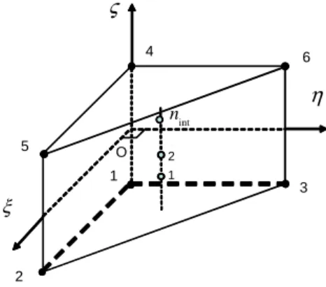
The SHB6 is a six-node prismatic continuum shell with only three displacement degrees of freedom per node. It is provided with a special direction called the “thickness”, normal to the mean plane of the triangle. A reduced integration scheme is adopted with a user-defined number n of integration points along the thickness int
(with a minimum of two) and only one point in the in-plane directions (see Figure 1). Accordingly, the element is intended to be used in structural problems (thin or moderately thick structures), where the special “thickness” direction of the element is set parallel to that of the structure that is being modeled.
Figure 1. Reference geometry of the SHB6 element, and its integration points … int n 1 2 ξ η ς 2 3 1 5 6 4 O
2.1. Kinematics and interpolation
The SHB6 is a linear, isoparametric element. Its spatial coordinates x and i
displacements u are respectively related to the nodal coordinates i x and iI
displacements u through the linear shape functions iI N=
(
N N1,
2,...,
N6)
as follows:( , , )
i iI I
x
=
x N
ξ η ζ
,u
i=
u N
iI I( , , )
ξ η ζ
[1]Above and hereafter, unless specified otherwise, the implied summation convention for repeated indices will be adopted. Lowercase indices i vary from one to three and represent spatial coordinate directions. Uppercase indices I vary from one to six and correspond to element nodes. The tri-linear isoparametric shape functions NI are:
(
)
(
)(
)
(
)
(
)
(
)(
)
(
)
(
)
[ ]
[
]
[ ]
1 1 1 0,1 1 1 , , , with 0,1 2 1 1 1,1 1 1 ζ ξ η ζ ξ ξ ζ η ξ η ζ η ξ ζ ξ η ζ ζ ξ ζ η − − − − = − = = − + − − = − + + N [2]2.2. Discrete gradient operator
Using some mathematical derivations, similarly to the procedure for the SHB8PS development (Abed-Meraim et al., 2009), we can explicitly express the relationship between the linear part of the strain field and the nodal displacements. Combining [1] and [2] leads to the following expansion for the displacement field:
(
)
0 1 2 3 1 1 2 2 1 2 , , , , , 1, 2, 3 , i i i i i i i u x y z a a x a y a z c h c h i h h ξ η ζ ζη ζξ = + + + + + = = =
[3]Evaluating this last equation at the element nodes yields the following three six-equation systems:
0 1 1 2 2 3 3 1 1 2 2 , 1, 2, 3 i =ai +ai +ai +ai +ci +ci i=
d s x x x h h [4]
where the six-component vectors d and i x respectively denote the nodal i displacements and coordinates, and vectors s and hα
(
α=1, 2)
are given by:1 2 ( 1, 1, 1, 1, 1, 1) (0, 0, 1, 0, 0,1) (0, 1, 0, 0,1, 0) T T T = = − = −
s h h [5]Let us now consider the derivatives of the shape functions evaluated at the origin of the reference frame:
, = = =0 ( ) 1, 2, 3 i i i Hallquist Form i x ξ η ζ ∂ = = = ∂ N b N 0 [6]
Explicit expressions of vectors b can be derived by algebra together with some i useful orthogonality relations:
0 , 0 , 0 , 2 , 1, ..., 3 , =1,2 T T T i i i j ij T T i j α α α β αβ α β δ δ ⋅ = ⋅ = ⋅ = ⋅ = ⋅ = =
b h b s b x h s h h [7]These orthogonality conditions allow the constants aki and cαi to be determined by scalar products: 3 1 1 where: ( ) 2
,
T T ki k i i i T j j j a cα α α α α = = ⋅ = ⋅ = − ⋅
∑
b d γ d γ h h x b [8]which, combined with [3], lead to the following convenient form for the displacement field:
0 ( 1 1 2 2 3 3 1 1 2 2)
T T T T T
i i i
u =a + xb +xb +xb +hγ +h γ ⋅d [9]
The strain field (i.e., symmetric part of the displacement gradient) is then obtained by differentiating this last equation:
( ) s
, , , , , , , , , , , , , , , , , , ( ) , , T T x x x x T T y y y y x T T z z z z s y T T T T x y y x y y x x T T T T z z z y y y z z y T T T T z z x x x z z x u h u h u h u h h h h u h h u
u
u
u
α α α α α α α α α α α α α α α α α α + + + ∇ = = = + + + + + + + + +
b γ 0 0 0 b γ 0 d 0 0 b γ u d d B b γ b γ 0 d 0 b γ b γ b γ 0 b γ
[11]This form of the discrete gradient operator B is very useful because it allows each of the non-constant strain modes to be handled separately to build an appropriate assumed-strain field. In addition, it can be shown that the γα vectors involved in this operator satisfy the following orthogonality relations:
0,
T T
j
α⋅ = α⋅ β =δαβ
γ x γ h [12]
These conditions will prove to be helpful in the subsequent analysis of stiffness matrix rank deficiencies.
2.3. Variational principle
The expression of the weak form of the Hu–Washizu mixed variational principle, as extended to nonlinear solid mechanics by Fish et al., (1988) reads for a single finite element:
(
)
( , , ) T T s( ) T ext 0
e e
v dv v dv
δπ v ε σ& =
∫
δε& ⋅σ +δ∫
σ ⋅ ∇ v −ε& −δd& ⋅f = [13] where δ denotes a variation, v the velocity gradient, ε& the assumed-strain rate, σ the interpolated stress, σ the stress evaluated by the constitutive equations, d& the nodal velocities, fext the external nodal forces, and ∇s( )v the symmetric part of the velocity gradient. In the simplified form of this principle, as described by Simo etal., (1986), the assumed stress field is chosen to be orthogonal to the difference
between the symmetric part of the velocity gradient and the assumed-strain rate, leading to:
( ) T T ext 0
e
v dv
Therefore, the discrete equations only require the interpolation of the displacement and the assumed-strain field. The latter is expressed in terms of a B matrix, projected starting from the standard B operator:
( , )x t = ( )x ⋅ ( )t
ε& B d& [15]
Replacing [15] in the variational principle [14], leads to the following expression for the internal forces:
( ) int T e v dv =
∫
⋅ f B σ ε& [16]This formulation is valid for problems involving nonlinear material models, in which σ is a function of the time history of the assumed-strain field and other internal state variables:
( , , ...)
=
σ F ε& αααα [17]
For linear elastic problems, the element stiffness matrix takes the following simple form: T e e v dv =
∫
⋅ ⋅ K B C B [18]Note that similarly to the SHB8PS element (Abed-Meraim et al., 2009), an improved plane-stress type constitutive law is adopted here, to enhance the element immunity with regard to thickness locking.
2.4. Hourglass mode analysis
Hourglass mechanisms are spurious zero-energy modes generated by the reduced integration. Therefore, the analysis of hourglass modes is equivalent to the investigation of stiffness matrix rank deficiency. Within a displacement-based approach, a zero-energy mode is a vector hg that satisfies:
int
1, ...,
(ζI)⋅ g = ; I = n
B h 0 [19]
We can easily demonstrate that the following
(
ei, i=1, ...,18)
vectors are linearly independent, and hence, they form a basis for the vector space of the discretized displacements:1 2 3 4 5 6 7 8 9 10 11 12 1 13 , , , , , , , , , , , , , = = = = = = = = = = = = =
h e 0 0 s 0 0 x 0 0 e 0 e s e 0 e 0 e x e 0 0 0 s 0 0 x y 0 0 z 0 0 e 0 e y e 0 e 0 e z e 0 0 0 y 0 0 z 2 14 1 15 16 17 2 18 1 2 , , , , = = = = =
0 0 h 0 0 e h e 0 e 0 e h e 0 0 h 0 0 h [20]Assuming that vector hg belongs to the stiffness kernel, one can expand it in terms of the above base vectors:
18 1 g i i i c = =
∑
h e [21]Combining [21], [19], and [11], and taking advantage of orthogonality conditions [7], one obtains:
( )
( )
( )
( )
( )
( )
( )
( )
( )
( )
( )
( )
( )
( )
( )
( )
( )
4 1, 13 2, 16 8 1, 14 2, 17 12 1, 15 2, 18 5 7 1, 13 1, 14 2, 16 2 , 17 9 11 1, 14 1, 15 2 , 17 2 , 18 6 10 1, 13 1, 15 2, 16 2 , I I I I I I I I I I I I I I I I I x x y y z z y x y x z y z y z x z x c h c h c c h c h c c h c h c c c h c h c h c h c c c h c h c h c h c c c h c h c h c h ζ ζ ζ ζ ζ ζ ζ ζ ζ ζ ζ ζ ζ ζ ζ ζ ζ ζ + + + + + + + + + + + + + + + + + + + + +( )
int 18 1, ..., , I I n c = =
0Evaluating the above equation at the n different integration points of the SHB6 int
implies that: 4 13 16 5 7 8 14 17 9 11 12 15 18 6 10 0 0 0 0 0 0
,
c c c c c c c c c c c c c c c = = = + = = = = + = = = = + =
[22] and hence:1 2 3 5 6 9 g c c c c c c − − = + + + + + −
s 0 0 y z 0 h 0 s 0 x 0 z 0 0 s 0 x y [23]This last equation reveals that the kernel of the stiffness matrix only consists of the usual six rigid body modes (three translations and three rotations), and thus no rank deficiency is observed. It should be noted that this formulation of the SHB6 element is valid for any set of n integration points located along the same line int
1
3, ,
I I I
ξ =η = ζ I =1, ...,nint, and comprising at least 2 integration points (nint ≥2).
2.5. Assumed-strain formulation for the SHB6
In this section, the discrete gradient operator B will be projected onto an appropriate subspace in order to eliminate different locking phenomena; the projected operator will be denoted B . It has been shown in the literature (see Simo
et al., 1986) that this assumed-strain method is consistent, from a variational
perspective, with the Hu–Washizu principle as long as the stress interpolation is appropriately chosen. However, this variational justification of the assumed-strain method does not provide a general and systematic way to derive adequate assumed-strain fields, and a specific analysis of locking must be conducted for each new element developed based on this approach. For this purpose, we propose a projection scheme that is both effective and simple (see Belytschko et al., (1993) for further details). In the contribution of Belytschko et al., (1993), two eight-node hexahedral elements named ASQBI and ADS were developed on the basis of specific projections. In a similar way, yet leading to a quite different projected operator B , the SHB8PS solid–shell formulation has been derived (Abed-Meraim et al., 2009). In the two contributions above, the additive split of the discrete gradient operator was primarily dictated by the hourglass part of the B operator. However, because the SHB6 element is shown to be free from spurious modes, the projection process is found here to be more difficult than for the eight-node counterpart. Taking advantage of the experience gained through the SHB8PS formulation, the discrete gradient operator B is first decomposed into two parts:
1 2
= +
B B B [24]
In this additive decomposition, the first part, B , contains the gradients in the 1 element mid-plane (membrane terms of the deformation) as well as the normal strains, whereas the second part, B , incorporates the gradients associated with the 2 transverse shear strains:
, , , 1 , , T T x x T T y y T T z z T T T T y y x x h h h h h α α α α α α α α α α + + + = + +
b γ 0 0 0 b γ 0 0 0 b γ B b γ b γ 0 0 0 0 0 0 0 [25] 2 , , , , T T T T z z y y T T T T z z x x h h h h α α α α α α α α = + + + +
0 0 0 0 0 0 0 0 0 B 0 0 0 0 b γ b γ b γ 0 b γ [26]Then, from numerical experiments, it is observed that the main locking effects in the SHB6 element originate from the transverse shears. Accordingly, we choose an integration scheme that enables us to reduce the associated fraction in the total strain energy. To this end, matrix B is projected as follows: 2
2 =ε 2
B B [27]
where ε is a shear scaling factor (0≤ ≤ε 1). By introducing the additive decomposition [24] of matrix B into [18] and making use of projection [27], the stiffness matrix becomes:
1 1 1 2 + 2 1 2 2 T T T T e e e e e v dv v dv v dv v dv =
∫
⋅ ⋅ +∫
⋅ ⋅∫
⋅ ⋅ +∫
⋅ ⋅ K B C B B C B B C B B C B [28]which can be simply written as: Ke =K1+K . The first term, 2 K , which is not 1 affected by projection, is evaluated at the integration points as defined above:
int 1 1 1 1 1 1 ( I) ( I) ( I) ( I) n T T e I v dv ω ζ Jζ ζ ζ = =
∫
⋅ ⋅ =∑
⋅ ⋅ K B C B B C B [29]The second term, K , embodies all the projection and reads: 2
2 1 2 2 1 2 2 T T T e e e v dv v dv v dv =
∫
⋅ ⋅ +∫
⋅ ⋅ +∫
⋅ ⋅ K B C B B C B B C B [30]The particular choice of the above additive decomposition [24] together with projection [27] yields a simplified form for the second part of the stiffness matrix
2
K . Indeed, with these choices the first two terms, i.e. cross-terms, in the right-hand side of [30] vanish, and matrix K simply reduces to: 2
2 2 2 T e v dv =
∫
⋅ ⋅ K B C B [31]Note that the extreme values of ε are 0 and 1 and correspond, respectively, to a vanishing B operator and to the absence of projection. In the first case (2 ε =0), no transverse shear strains are taken into account, which not only is likely to lead to improper results, but also to hourglass mechanisms and singularity of the stiffness matrix. The second case (ε =1) corresponds to the absence of projection, and the associated unmodified SHB6 version (i.e., without assumed-strain projection) is shown to be much less accurate than that using projection (see the benchmark tests presented in the next section).
The identification of the shear scaling factor ε in [27] has been carried out through numerical experiments, and the selected value for this parameter is found to be one half. This value is motivated by extensive testing on a variety of linear and nonlinear popular test problems. Although not physically motivated, this choice of projection leads to reasonably good behavior for the element in most of the representative benchmark problems that have been tested.
2.6. Geometric stiffness matrix
In this section, the geometric stiffness matrix for the SHB6 element is derived. For instance, this geometric stiffness matrix Kσσσσ has to be added to the regular tangent stiffness matrix K in a usual structural stability analysis. Note that the e geometric stiffness matrix originates from the linearization of the virtual work principle and is due to the nonlinear (quadratic) part of the strain tensor. In its continuum form, it reads:
(
,)
: T : Q(
)
e e v v δu ∆u =∫
δu ⋅ ∆udv=∫
e δ ,u ∆u dv σσσσ σ ∇σ ∇σ ∇σ ∇ ∇∇∇∇ σσσσ K [32]Making use of the vector form of the stress tensor and the quadratic part of the strain tensor, respectively, Equation [32] can be rewritten as:
(
,)
Q(
,)
e v δu ∆u =∫
Τ ⋅e δu ∆u dv σσσσ σσσσ K [33] with:, Q xx xx Q yy yy Q zz Q zz Q Q xy xy yx Q Q yz yz zy Q Q xz xz zx e e e e e e e e e σ σ σ σ σ σ = = + + +
e σσσσ [34]and the components of the quadratic part of the strain tensor are given by:
(
)
3 , , , , 1 Q ij k i k j k i k j k e δ ,δ
u
u δu u = ∆ =∑
∆ = ∆ u u [35]Using the discrete form of the displacement gradient, as given in Equation [11], one obtains:
(
)
(
)
, , , , T T T i i k i k T T T k j j j k j k k i u h u h α α α α δ = + ⋅δ = ⋅δ ∆ = + ⋅ ∆ = ⋅ ∆
b γ d B d b γ d B d [36]The components of the nonlinear part of the strain tensor can be discretized as:
(
)
(
)(
)
1 1 2 2 3 3 3 1 , where: , , Q T T T Q k i j k T i j Q T i j T i j ij ij k ij e δ δ δ δ δ δ δ = ∆ = ⋅ ⋅ ∆ = ⋅ ⋅ ∆ ∆ = = ∆ = ∆ ∆
∑
u u d B B d d B d d d B B 0 0 B 0 B B 0 d d d d 0 0 B B d d [37]With these quadratic discrete gradient operators BQij, the contribution kσσσσ
( )
ζI atintegration point ζI to the overall geometric stiffness matrix is given by:
( )
( ) ( )
( ) ( )
( ) ( )
( )
(
( )
( )
)
( )
(
( )
( )
)
( )
(
( )
( )
)
I I I I I I I I I I I I I I I I Q Q Q xx yy zz Q Q Q Q xy yz Q Q xz xx yy zz xy yx yz zy xz zx ζ ζ ζ ζ ζ ζ ζ ζ ζ ζ ζ ζ ζ ζ ζ ζ σ σ σ σ σ σ = + + + + + + + + k B B B B B B B B B σσσσ [38]The geometric stiffness matrix is finally obtained using the integration points as:
( )
int 1 ( ) ( ) I n I I I J ζ ω ζ ζ = =∑
Kσσσσ kσσσσ [39]2.7. Numerical aspects for nonlinear analyses
In this section, the main features of the implementation of the SHB6 element are briefly described. For this purpose, the incremental, nonlinear, and implicit finite element code ASTER has been used. In this process, the updated Lagrangian strategy is adopted. For the stress and internal variable updates, the well-known co-rotational formulation is used. The equilibrium equations are solved step-by-step using an iterative procedure based on the Newton–Raphson scheme. These iterations are performed until the residual load vector is sufficiently small, using a constant tangent stiffness matrix built at the beginning of the current time step. For structural instability problems involving either a load-limit point (snap-through) or a deflection-limit point (snap-back), as well as for material instability (softening behavior), the path-following Riks algorithm, which is based on an arc-length control parameter (Riks, 1979), is adopted.
For coupling with nonlinear behavior models, an elastic–plastic constitutive law with isotropic hardening and associative plastic flow rule has been used. As previously mentioned, the standard three-dimensional elastic constitutive law has been specifically modified for this element formulation, and this must accordingly be taken into account for the time integration of the set of constitutive equations. This is the main modification with respect to the classical radial return mapping algorithm based on Newton–Raphson’s iterative procedure. The associated yield criterion is defined by:
( )
p 0eq y
F =σ −σ ε ≤ [40]
where σeq is the von Mises equivalent stress and σy is the yield stress, which can be described by a nonlinear function of the equivalent plastic strain εp. Note that for isotropic hardening, Equation [40] can be regarded as a geometric transformation for the yield surface, in which this surface, whose current size is σy, expands homogenously without distortion in stress space.
3. Evaluation on benchmark problems
In this section, the evaluation of the SHB6 element will be carried out through several popular linear and nonlinear benchmark problems. For each test problem, the
obtained results are compared with the reference solution from the literature, and when relevant, they are additionally compared with either the solutions given by both the standard three-dimensional six-node prism element PRI6 and the unmodified SHB6 element (i.e., without assumed-strain projection), or those yielded by the hexahedral solid–shell element SHB8PS. For the sake of clarity, the assumed-strain projected version of the SHB6 will be denoted SHB6bar. The first preliminary linear test problems are mainly intended to assess the performance of the element in bending-dominated problems and to illustrate the benefit of mixing hexahedral and prismatic solid–shell elements such as the SHB6bar and SHB8PS. In all numerical tests, a single element is used through the thickness, unless prescription of boundary conditions requires using two layers of FE. For elastic problems, only two integration points are used, whereas for elastic–plastic tests, five integration points are used through the thickness. In the reported results, the meshes are indicated by the number of subdivisions in each direction (length, width), and the total element number is then doubled, since each rectangle is divided into two triangles.
3.1. Buckling of a cylinder under external pressure
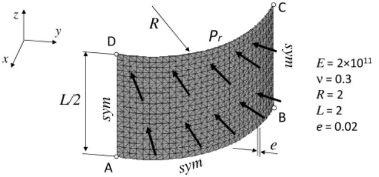
In this test, a linear stability analysis of a thin cylinder, which is free at its ends and subjected to a uniformly distributed external pressure, is carried out. This problem also allows the verification of the formulation of the geometric stiffness matrix Kσσσσ. Indeed, in this linear buckling analysis, the Euler critical pressure is determined along with the corresponding buckling mode. This critical state is associated with the lowest pressure that makes the global stiffness matrix singular and is classically obtained by solving the eigenvalue problem:
(
Ke+λcKσσσσ)
⋅Xc =0 [41]in which
λ
c is the critical buckling load and Xc is the associated buckling mode. The geometric and material parameters are shown in Figure 2.x y z L/2 R e sy m sy m A B C D
P
r E = 2×10¹¹ ν= 0.3 R = 2 L = 2 e = 0.02The reference solutions used for comparison are analytical, given by (Timoshenko et al., 1966; Brush et al., 1975). Owing to the symmetry, only one eighth of the cylinder is modeled, and symmetry boundary conditions are applied, which in turn restrict the analysis to symmetric buckling modes (i.e., modes 2, 4 and 6 as shown in Figure 3). The corresponding critical pressure Pcr is given by the analytical expression: Pcr =En2 12 1
(
−ν2)
(
e R)
3, with n=2, 4, 6.L/2 R e sy m sy m A B C D Mode 2 L/2 R e sy m sy m A B C D Mode 4 L/2 R e sy m sy m A B C D Mode 6
Figure 3. Buckling modes n° 2, 4 and 6; a (20×30×1)×2 mesh using SHB6 elements
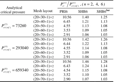
The results obtained for the three modes (n=2, 4 and 6 ) are reported in Table 1 in terms of critical pressure, normalized with respect to the analytical solution. These reveal that the assumed-strain version SHB6bar has a better convergence rate than the SHB6 and PRI6 elements, and represents a significantly improved alternative to the PRI6, which exhibits locking and very slow convergence rate.
Table 1. Normalized critical pressure for the thin cylinder under uniform pressure
Analytical
critical pressure Mesh layout
( ) ( ) ( ) n n cr cr ref
P
P
, (n
=
2, 4, 6
) PRI6 SHB6 SHB6bar (2) ( )73260
cr refP
=
(20×30×1)×2 10.56 1.40 1.25 (20×40×1)×2 6.45 1.21 1.13 (20×50×1)×2 4.55 1.13 1.08 (20×60×1)×2 3.53 1.09 1.05 (20×70×1)×2 2.91 1.06 1.03 ( 4) ( )293040
cr refP
=
(20×30×1)×2 10.56 1.42 1.26 (20×40×1)×2 6.44 1.22 1.13 (20×50×1)×2 4.55 1.14 1.08 (20×60×1)×2 3.52 1.09 1.05 (20×70×1)×2 2.91 1.06 1.03 (6) ( )659340
cr refP
=
(20×30×1)×2 10.56 1.46 1.28 (20×40×1)×2 6.43 1.24 1.14 (20×50×1)×2 4.54 1.15 1.08 (20×60×1)×2 3.52 1.10 1.05 (20×70×1)×2 2.90 1.07 1.033.2. Pinched hemispherical shell with mixed hexahedral and prismatic FE
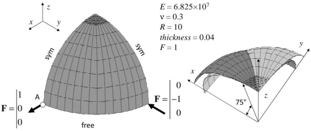
This test problem, which is often used to assess the three-dimensional inextensional bending behavior of shells, has become very popular and has been adopted by many authors since it was proposed by MacNeal et al., (1985). Figure 4 shows the geometry, loading, and boundary conditions for this elastic thin shell problem (R/t = 250). In this example, a mixture of SHB6 and SHB8PS elements is used, in which the SHB6 elements are located at the top of the hemisphere.
free A 1 0 0 = F 0 1 0 = − F x y z E = 6.825×10⁷ ν= 0.3 R = 10 thickness = 0.04 F = 1 x y z 75°
a) Test geometry and loading b) Initial and deformed configurations
Figure 4. Pinched hemispherical shell problem with a mixture of prismatic and hexahedral elements: the SHB6 elements are located at the top, and the SHB8PS elements are arranged over an angle of 75°
Owing to the symmetry of the test, only one quarter of the hemisphere is meshed using a single layer of elements through the thickness and with two unit loads along the directions Ox and Oy. According to the reference solution (MacNeal et al., 1985;
Trinh et al., 2011), the displacement of point A along the x-direction is w = ref
0.0924. Note that in order to compare the performance of solid–shell elements to that of standard three-dimensional elements, SHB6 elements are mixed with SHB8PS elements, and PRI6 elements are mixed with their three-dimensional counterpart HEX8, which are the standard, full integration eight-node hexahedral elements. The normalized results reported in Table 2 reveal a very good convergence rate when the SHB6bar is mixed with the SHB8PS, whereas the conventional linear solid elements show too stiff behavior in this test problem. This confirms the interest of mixing hexahedral and prismatic solid–shell elements.
Table 2. Normalized displacements at point A for the pinched hemispherical shell problem: mixed meshes
Number of elements PRI6 + HEX8 SHB6 + SHB8PS SHB6bar + SHB8PS ref w w w wref w wref 36 0.001 0.703 0.785 100 0.002 0.880 0.960 156 0.004 0.929 0.983
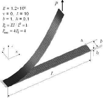
3.3. Cantilever beam subjected to a conservative end shear force
This problem has been widely used by many investigators and considered as a benchmark test for large deflection analysis (see e.g., Sze et al., (2004), among others). Figure 5 gives the geometric and material properties as well as an example of mesh using SHB6 elements. One end of this thin beam is clamped and the other is subjected to a vertical shear force. An accurate reference solution was tabulated by
Sze et al., (2004), which was obtained by means of the Abaqus shell element S4R
with a converged mesh of 16×1 elements.
Figure 5. Cantilever subjected to end shear force: example of a (100×10×1)×2 mesh with SHB6 elements; initial and deformed configuration under maximum force
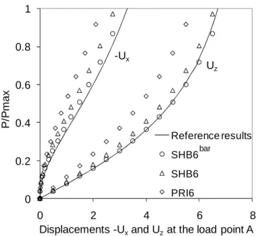
Figure 6 shows the normalized load–deflection curves obtained with different finite elements. For the same mesh (100×10×1)×2, with a single element through the thickness, the results given by the SHB6bar, SHB6 and PRI6 are compared to the reference solution. One can observe that the plots given by the SHB6bar element are the closest to the reference solution, while the two other elements (especially the PRI6) show a stiffer response in this test problem.
0 0.2 0.4 0.6 0.8 1 0 2 4 6 8 P /P m a x
Displacements -Uxand Uzat the load point A Reference results SHB6_bar SHB6 PRI6 -Ux Uz bar
Figure 6. Cantilever beam subjected to end shear force: normalized end shear load versus the displacements of the load point A along the directions Ox and Oz
3.4. Pull-out of an open-ended cylindrical shell
This test problem consists of an elastic thin cylindrical shell with free edges subjected to a pair of diametrically opposite radial forces. The geometric and material properties as well as the boundary conditions and loading are described in Figure 7. Only one octant of the cylinder is modeled, due to the symmetry, with a single element along the thickness.
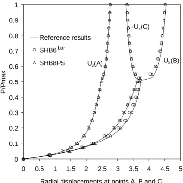
The reference results for this test were given by Sze et al., (2004), using the
Abaqus shell element S4R with a converged mesh of 24×36 elements. The results shown in Figure 8 correspond to the following meshes: 24×36 S4R, (45×45×1)×2
SHB6bar, and 20×30×1 SHB8PS elements, and represent the normalized load versus the radial displacements at points A, B, and C. These reveal that the results of the proposed solid–shell elements are in good agreement with the reference solution.
sym sym L A B C free free x y z R P E= 10.5×10⁶ ν= 0.3125 R= 4.953 L= 10.35 thickness = 0.094 Pmax= 40,000
Figure 7. Description of the open-ended cylindrical shell benchmark test: example of mesh with 20×30×1 SHB8PS elements for one octant of the cylinder
0 0.1 0.2 0.3 0.4 0.5 0.6 0.7 0.8 0.9 1 0 0.5 1 1.5 2 2.5 3 3.5 4 4.5 5 P /P m a x
Radial displacements at points A, B and C Reference results SHB6 SHB8PS Uz(A) -Ux(C) -Ux(B) bar
Figure 8. Normalized load–deflection results for the open-ended cylindrical shell test: comparison between the proposed solid–shell FE and the reference solution
3.5. Snap-through and snap-back instability of a thin elastic panel
This is a popular benchmark test that has been widely considered in the literature (see e.g., Sze et al., (2004), Killpack et al., (2011), Leahu-Aluas et al., (2011),
among many others). Figure 9 shows the initial and deformed configurations, geometric and materials properties, boundary conditions and loading. Owing to the symmetry, only one quarter of the structure is modeled.
R A h sym hin ged sym free P L α B C D initial configuration deformed configuration initial configuration deformed configuration R = 2540 L = 254 h = 6.35 α= 0.1 E = 3102.75 ν= 0.3 x y z
Figure 9. Hinged thin cylindrical section subjected to a central concentrated load: geometric and material properties as well as initial and deformed configurations
-0.2 -0.1 0 0.1 0.2 0.3 0.4 0.5 0.6 0.7 0 5 10 15 20 25 30 35 40 P /P m a x
Vertical displacement at the load point A Reference results SHB6
SHB8PS bar
Figure 10. Normalized load–displacement curves at the load point A for the hinged thin cylindrical section subjected to a central concentrated load
The panel is hinged at its edge BC (mid-surface of the panel), free at its edge CD, and subjected to a concentrated force P at point A along the vertical direction Oz (see Figure 9). It is noteworthy that this test is very sensitive to the particular
location of the prescribed boundary conditions (mid-surface, upper or lower edge), and the corresponding responses show significant differences. Therefore, to reproduce shell boundary conditions (i.e., on the mid-surface), two layers of 3D elements need to be used along the thickness. Also, to be able to capture the snap-through behavior and to follow the curve beyond the limit-point, the Riks path-following strategy has been adopted (Riks, 1979). The results plotted in Figure 10 correspond to the following discretizations: (25×25×2)×2 SHB6bar, 20×20×2 SHB8PS, and 24×24 S4R elements; the latter represent the converged mesh providing the reference solution (Sze et al., 2004). This comparison reveals that the
SHB6bar results are in very good agreement with the reference solution.
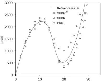
3.6. Limit-point buckling of a thick elastic panel
This test is the same as the previous one with the exception of the thickness, which is now twice as large (h = 12.7). Similarly to its thin counterpart, this
nonlinear benchmark problem has been extensively investigated in the literature. The geometry, material properties, boundary conditions and loading can be seen again in Figure 9. Also, by virtue of symmetry, only a quarter of the panel is modeled for the finite element simulations. Two layers of three-dimensional elements need to be used along the thickness of the panel, so that the prescribed shell boundary conditions can be consistently reproduced. In the same way, the solution procedure makes use of the Riks path-following strategy, which enables both to predict the snap-through behavior of the structure and to follow the curve beyond the limit-point.
For this test problem, an accurate reference solution has been given by Sze et al.,
(2004), using the Abaqus shell element S4R with a converged mesh of 24×24 elements. Therefore, the three prismatic finite elements (i.e., SHB6bar, SHB6and PRI6) can be compared to this reference solution. The obtained results are shown in Figure 11 in terms of plots of the applied load versus the vertical displacement at the load point A. These correspond to the following meshes: 24×24 S4R (for the
reference solution), and (30×30×2)×2 for the three elements SHB6bar, SHB6 and PRI6. Again, it can be seen from Figure 11 that the results given by the proposed solid–shell are in better agreement with the reference solution than those yielded by the PRI6 element.
0 500 1000 1500 2000 2500 3000 0 10 20 30 L o a d
Vertical displacement at the load point A
Reference results SHB6 bar SHB6 PRI6
bar
Figure 11. Load–displacement curves at the load point A for the hinged thick cylindrical section subjected to a central concentrated load
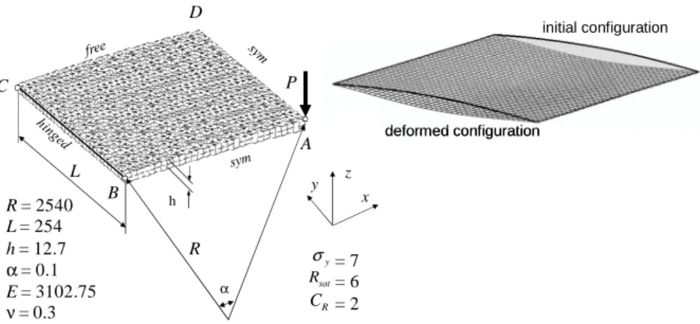
3.7. Elastic–plastic buckling of a thick cylindrical panel
The elastic version of this test having been analysed in the previous section, we consider here an elastic–plastic version in which both types of nonlinearities, geometric and material, are included. For this new elastic–plastic benchmark test, we had first to build the associated reference solution. The latter was obtained using Abaqus S4R5 shell elements, for which convergence was achieved with a mesh of 20×20 elements. The geometric and material parameters are given in Figure 12. The elastic–plastic constitutive equations correspond to the Voce nonlinear saturating isotropic hardening law, which is associated with the von Mises yield surface
0 eq
F =σ − ≤Y such that: Y =σy+Rsat
(
1 exp(− −CRε p))
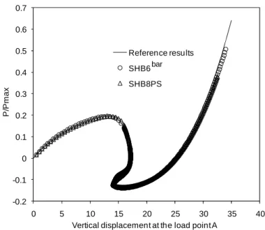
, where σy is the initial yield stress, Rsat, C the material parameters, and R ε p the equivalent plastic strain.Owing to the symmetry, only one quarter of the structure is modeled. The lateral, straight sides are hinged, while the two other curved sides are free. As discussed before, two layers of 3D elements are used along the thickness in order to reproduce shell boundary conditions, and the Riks path-following strategy is adopted to follow the curve beyond the limit-point. The results shown in Figure 13 correspond to the following meshes: 20×20 S4R5, (20×20×2)×2 SHB6bar, and 15×15×2 SHB8PS finite elements. In Figure 13, the applied load is plotted versus the vertical displacement at the load point A. It can be observed that the elastic–plastic behavior
decreases the first limit load, which is here about 75% of its elastic value. These results are in good agreement with the reference solution obtained with Abaqus S4R5 shell elements, which confirms the ability of the proposed solid–shell finite element to predict such critical points and the associated post-buckling response.
R A h P L α B C x y z D R = 2540 L = 254 h = 12.7 α= 0.1 E = 3102.75 ν= 0.3 = 7 = 6 = 2 y σ sat R R C initial configuration deformed configuration initial configuration deformed configuration
Figure 12. Description of the thick elastic–plastic panel benchmark problem;
example of mesh with (30×30×2)×2 SHB6 elements for one quarter of the panel
0 500 1000 1500 2000 2500 3000 0 10 20 30 40 L o a d
Vertical displacement at the load point A Reference results SHB6
SHB8PS bar
Figure 13. Load–deflection results for the thick elastic–plastic panel: comparison between the proposed solid–shell finite elements and the reference solution
4. Discussion and conclusions
A new solid–shell element SHB6bar has been developed and implemented into the finite element code ASTER. The key idea of this development is the adequate combination of a reduced integration rule with the well-known assumed-strain method. An interesting feature of this approach is the convenient fully three-dimensional framework on which this solid–shell element is based (six-node prism with only three translational degrees of freedom per node). Also it has been shown that no zero-energy modes arise from the adopted reduced integration scheme, and thus no stabilization procedure is required. As revealed by the benchmark problems, the SHB6bar element brings significant improvements compared to the standard three-dimensional six-node prismatic element denoted PRI6. The projection using the assumed-strain technique makes the quality of the element even better under combined bending and shearing. This type of element blends naturally with the eight-node hexahedral solid–shell element SHB8PS, thus enabling one to analyze any structural geometry quite easily, which is the main motivation behind the development of the present SHB6bar element. Recall that meshing arbitrarily complex geometries is not permitted using only hexahedral elements. Due to the better performance of quadrangular-based elements, it is advisable to mesh with SHB8PS solid–shell elements, wherever possible, and to keep the SHB6 element for the only purpose of completing the meshes.
Acknowledgements
The authors would like to thank EDF for its funding to this project. The financial support from CETIM is also gratefully acknowledged.
5. References
Abed-Meraim F., Combescure A., “SHB8PS – a new adaptive, assumed-strain continuum mechanics shell element for impact analysis”, Computers & Structures, vol. 80, 2002, p. 791-803.
Abed-Meraim F., Combescure A., “An improved assumed strain solid–shell element formulation with physical stabilization for geometric nonlinear applications and elastic-plastic stability analysis”, International Journal for Numerical Methods in Engineering, vol. 80, 2009, p. 1640-1686.
Belytschko T., Bindeman L.P., “Assumed strain stabilization of the eight node hexahedral element”, Computer Methods in Applied Mechanics and Eng., vol. 105, 1993, p. 225-260. Brush D.O., Almroth B.O., Buckling of bars, plates and shells, McGraw-Hill, New York,
Dvorkin E.N., Bathe K.-J., “Continuum mechanics based four-node shell element for general non-linear analysis”, Engineering Computations, vol. 1, 1984, p. 77-88.
Fish J., Belytschko T., “Elements with embedded localization zones for large deformation problems”, Computers & Structures, vol. 30, 1988, p. 247-256.
Hauptmann R., Schweizerhof K., “A systematic development of solid-shell element formulations for linear and non-linear analyses employing only displacement degrees of freedom”, International Journal for Numerical Methods in Eng., vol. 42, 1998, p. 49-69. Killpack M., Abed-Meraim F., “Limit-point buckling analyses using solid, shell and solid–
shell elements”, Journal of Mechanical Science and Technology, vol. 25, 2011, p. 1105-1117.
Klinkel S., Gruttmann F., Wagner W., “A continuum based three-dimensional shell element for laminated structures”, Computers & Structures, vol. 71, 1999, p. 43-62.
Klinkel S., Wagner W., “A geometrical non-linear brick element based on the EAS-method”,
International Journal for Numerical Methods in Engineering, vol. 40, 1997, p. 4529-4545.
Leahu-Aluas I., Abed-Meraim F., “A proposed set of popular limit-point buckling benchmark problems”, Structural Engineering and Mechanics, vol. 38, 2011, p. 767-802.
Legay A., Combescure A., “Elastoplastic stability analysis of shells using the physically stabilized finite element SHB8PS”, International Journal for Numerical Methods in
Engineering, vol. 57, 2003, p. 1299-1322.
MacNeal R.H., Harder R.L., “A proposed standard set of problems to test finite element accuracy”, Finite Elements in Analysis and Design, vol. 1, 1985, p. 3-20.
Puso M.A., “A highly efficient enhanced assumed strain physically stabilized hexahedral element”, International Journal for Numerical Meth. in Eng., vol. 49, 2000, p. 1029-1064. Reese S., Wriggers P., Reddy B.D., “A new locking-free brick element technique for large deformation problems in elasticity”, Computers & Structures, vol. 75, 2000, p. 291-304. Riks E., “An incremental approach to the solution of snapping and buckling problems”,
International Journal for Numerical Methods in Engineering, vol. 15, 1979, p. 524-551.
Simo J.C., Armero F., “Geometrically non-linear enhanced strain mixed methods and the method of incompatible modes”, International Journal for Numerical Methods in
Engineering, vol. 33, 1992, p. 1413-1449.
Simo J.C., Armero F., Taylor R.L., “Improved versions of assumed enhanced strain tri-linear elements for 3D finite deformation problems”, Computer Methods in Applied Mechanics
and Engineering, vol. 110, 1993, p. 359-386.
Simo J.C., Hughes T.J.R., “On the variational foundations of assumed strain methods”,
Journal of Applied Mechanics, ASME, vol. 53, 1986, p. 51-54.
Simo J.C., Rifai M.S., “A class of mixed assumed strain methods and the method of incompatible modes”, International Journal for Numerical Methods in Engineering, vol. 29, 1990, p. 1595-1638.
Sze K.Y., Liu X.H., Lo S.H., “Popular benchmark problems for geometric nonlinear analysis of shells”, Finite Elements in Analysis and Design, vol. 40, 2004, p. 1551-1569.
Timoshenko S.P., Gere J.M., Théorie de la stabilité élastique, 2nd edition, Dunod, 1966.
Trinh V.D., Abed-Meraim F., Combescure A., “A new assumed strain solid–shell formulation “SHB6” for the six-node prismatic finite element”, Journal of Mechanical Science and
Technology, vol. 25, 2011, p. 2345-2364.
Wall W.A., Bischoff M., Ramm E., “A deformation dependent stabilization technique, exemplified by EAS elements at large strains”, Computer Methods in Applied Mechanics
and Engineering, vol. 188, 2000, p. 859-871.
Wriggers P., Reese S., “A note on enhanced strain methods for large deformations”,
Computer Methods in Applied Mechanics and Engineering, vol. 135, 1996, p. 201-209.
Zhu Y.Y., Cescotto S., “Unified and mixed formulation of the 8-node hexahedral elements by assumed strain method”, Computer Methods in Applied Mechanics and Engineering, vol. 129, 1996, p. 177-209.