is an open access repository that collects the work of Arts et Métiers Institute of
Technology researchers and makes it freely available over the web where possible.
This is an author-deposited version published in: https://sam.ensam.eu
Handle ID: .http://hdl.handle.net/10985/10555
To cite this version :
Thomas HENNERON, Stéphane CLENET - Application of the PGD and DEIM to solve a 3D Non-Linear Magnetostatic Problem coupled with the Circuit Equations - IEEE transactions on
Magnetics - Vol. 52, n°3, p.1-4 - 2015
Any correspondence concerning this service should be sent to the repository Administrator : archiveouverte@ensam.eu
Application of the PGD and DEIM to solve a 3D Non-Linear
Magnetostatic Problem coupled with the Circuit Equations
T. Henneron
1, S. Clénet
21 L2EP, Université Lille 1, 59655 Villeneuve d’Ascq, France 2L2EP, Arts et Métiers ParisTech, 59046 Lille, France
Among the model order reduction techniques, the Proper Generalized Decomposition (PGD) has shown its efficiency to solve static and quasistatic problems in the time domain. However, the introduction of nonlinearity due to ferromagnetic materials for example has never been addressed. In this paper, the PGD technique combined with the Discrete Empirical Interpolation Method (DEIM) is applied to solve a non-linear problem in magnetostatic coupled with the circuit equations. To evaluate the reduction technique, the transient state of a three phase transformer at no load is studied using the full Finite Element model and the PGD_DEIM model.
Index Terms—Proper Generalized Decomposition, Empirical Interpolation Method, Non-Linear magnetostatic problem
I. INTRODUCTION
O reduce the computation time of time-dependent numerical models, Model Order Reduction (MOR) methods have been developed and presented in the literature. These methods consist in searching a solution in a subspace of the approximation space of the full numerical model [1][2]. They have been mainly used to solve problems in mechanics. In this field, the Proper Generalized Decomposition (PGD) method has been developed since the early 2000’s and knows an increasing interest in the scientific community [3][4]. For problems in the time domain, the PGD method consists in approximating the solution by a sum of separable functions in time and space, so-called modes. Each mode is determined by an iterative procedure and depends on the previous modes. In the case of non-linear problems, the MOR methods are not so efficient than in the linear case, due to the computation cost of the non-linear terms. In fact, the calculation of the non-linear terms of the reduced model requires the calculation of the non-linear vectors or/and matrices of the full model. To circumvent this issue, the Discrete Empirical Interpolation Method (DEIM) method can be used [5][6]. This method consists in interpolating the non-linear terms of the full model by calculating only some of their entries. In the literature, the PGD approach has been combined with the DEIM in order to solve a thermal problem with a quadratic nonlinearity [7]. In computational electromagnetics, the PGD approach has been developed to study a fuel cell polymeric membrane model [8]. In static electromagnetism, the behavior of a Soft Magnetic Composite Material has been modeled [9]. In the case of magneto-quasistatics, the skin effect in a rectangular slot or in a conducting plate has been addressed [10][11]. However, any non-linear problem has not been solved using the PGD combined with the DEIM in computational electromagnetics.
In this paper, we propose to apply the PGD_DEIM approach to solve a 3D non-linear magnetostatic problem coupled with multiple external electric circuits using the vector potential formulation. First, the non-linear magnetostatic problem coupled with electric circuits is presented. Secondly, the PGD_DEIM approach is developed.
Finally, a three phase transformer at no load is studied in the case of a sinusoidal supply and also with a PWM supply. The results obtained with the PGD_DEIM model are compared in terms of accuracy and computation time with the full model.
II. NON-LINEAR MAGNETOSTATIC PROBLEM COUPLED WITH ELECTRIC CIRCUIT EQUATIONS
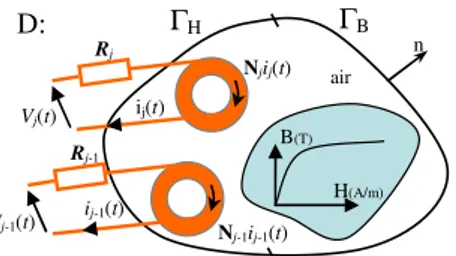
Let us consider a domain D of boundary Γ (Γ=ΓB∪ΓH and
ΓB∩ΓH=0) (Fig. 1). The problem is solved on D×[0,T] with T the width of the time interval. The eddy current effect is neglected however several stranded inductors are considered.
ΓB D: B(T) H(A/m) air Vj(t) Njij(t) ij(t) Rj n Vj-1(t) N j-1ij-1(t) ij-1(t) Rj-1 ΓH
Fig. 1. Non-linear magnetostatic problem coupled with electric circuits
In the case of magnetostatics, the problem can be described by the following equations:
∑
= = st N j j j i t t 1 ) ( ) ( ) , (x N x H curl div B(x, t) = 0 H(x,t) = ν(B) (x)B(x, t) (1) (2) (3) where B is the magnetic flux density, H the magnetic field, Njthe unit current density vector and ij the current flowing through the jth stranded inductor, Nst is the number of inductors and ν(B)(x) is the reluctivity which depends on B in the
ferromagnetic part. To impose the uniqueness of the solution, boundary conditions are introduced such that:
B(x, t)⋅n=0 on ΓB and H(x, t)×n=0 on ΓH (4)
with n the outward unit normal vector. In order to impose the voltage at the terminals of the stranded inductors, the following relations are added:
st j j j j N j t v t i R t Φ .., 1, with ) ( ) ( dt ) ( d = = + (5)
where Rj is the resistance, Φj the flux linkage and vj the voltage of the jth inductor. To solve the problem, the vector potential formulation is introduced. The vector potential A is defined such that B(x, t)=curl A(x, t) with A(x, t)××××n=0 on ΓB.
To take into account the non-linear behavior of the ferromagnetic materials, the magnetic field H(x, t) is defined by H(x, t)=νfpB(x, t)+Hfp(B(x, t)) with νfp a constant and Hfp(B(x, t))=(ν(B)(x) - νfp)B(x, t) a virtual magnetization
vector. In the materials with a constant reluctivity ν, the same expression can be used with νfp =ν and Hfp(B(x, t))=0. To
determine a solution to the problem on D×[0,T], weak forms of (1) and (5) can be written such that:
∫ ∫
∫ ∫ ∑
∫ ∫
⋅ = ⋅ − ⋅ = T T N j j j T t t t t t t i t t t st 0 D fp 0 D 1 0 D fp )dDd , ( ' )) , ( ( )dDd , ( ' ) ( ) ( )dDd , ( ' ) , ( x A curl x A curl H x A x N x A curl x A curl ν (6) 1,.., )d ( ) ( (t)dt i' ) ( )dD ( ) , ( d d T 0 0 D st ' j j T j j j Ri t v t i t t j N t t ⋅ = ⋅ = + ⋅ ∫ ∫ ∫Ax N x (7)with A’(x, t) and ij’(t) test functions which belong to the same functional spaces as A(x, t)and ij(t) respectively.
III. MODEL ORDER REDUCTION
A. Proper Generalized Decomposition
To solve (6) and (7), the PGD method can be applied. The vector potential A(x, t)is then approximated by a separated representation of space and time functions,
∑
= ≈ M j j j S t t 1 ) ( ) ( ) , (x R x A (8)with M the number of modes of the expansion. The terms
Rn(x), Sn(t) and the currents il(t)1≤l≤Nst in the Nst stranded inductors, are calculated iteratively. At the nth iteration, the approximation of the solution is An(x, t) = Rn(x)Sn(t)+An-1(x, t) with Rn(x) and Sn(t) the functions to determine belonging to
L2curl(D) and L2([0,T]) and An-1(x,t) the approximation determined during the previous n-1 iterations. In (6), A(x, t) is replaced by its approximation An(x, t). The test function is
given by A’(x, t)= R’n(x)Sn(t)+Rn(x)S’n(t) with R’n(x) and S’n(t) test functions belonging to the same spaces as Rn(x) and Sn(t). To calculate Rn(x), Sn(t) and in(t)1≤n≤Nst, two sets of
equations deduced from weak forms (6) and (7), are solved iteratively. First, we suppose that Sn(t) and in(t)1≤n≤Nst are
known. Then, the test function becomes A’(x, t)=R’n(x)Sn(t) and Rn(x) is the solution of the weak formulation,
∫
∫
∫
∫
∫
∫
∑
∫
∫
⋅ − = ⋅ − = ⋅ = ⋅ = + + ⋅ = ⋅ − − − − = T n n n T n 1 -n n T n j Rj T n n R N j n j Rj R t t t S t t t S t t S t i B t t S t S A B A st 0 D fp NL R 0 D fp L R 0 0 NL R L R 1 D D fp )dDd ( ' )) , ( ( ) ( , )dDd ( ' ) , ( ) ( , )d ( ) ( , )d ( ) ( with )dD ( ' ) ( )dD ( ' ) ( x R curl x A curl H F x R curl x A curl F F F x R curl x N x R curl x R curl ν ν (9)In (9), the term Rn(x) is a function of Sn(t) and il(t)1≤l≤Nst. We
denote λ the operator such that Rn(x)=λ(Sn(t), il(t)1≤l≤Nst).
Secondly, to calculate the function Sn(t) and update the currents il(t)1≤l≤Nst, we assume that the function Rn(x) is known. In this case, the test function in (6) is equal to
R’n(x)Sn(t). Considering (6) and (7), it can be shown that the functions Sn(t) and il(t)1≤l≤Nst are solutions of the following
Ordinary Differential Equation (ODE) systems:
{
}
∫
∑
∫
∑
∫
∫
∫
∑
⋅ = ⋅ − = ⋅ − = ⋅ = ⋅ = ∈ + = + + = − − = − = − − − = D fp 1 D fp 1 D j D D fp 1 )dD ( )) , ( ( , )dD ( ) ( ν ) ( )dD ( ) ( d ) ( d , )dD ( ) ( , )dD ( ) ( ν with ,..., ) ( d ) ( d ) ( ) ( ) ( x R curl x A curl H x R curl x R curl x R x N x R x N x R curl x R curl n n NL S 1 -n j n j j L S 1 -n j k j k i n k Sk n n S st k -i k n Sk k k NL S L S k N k Sk n S t F t S F t t S F B A N 1 k F t v t t S B t i R F F t i B t S A st (10)Again, we define γ an operator such that (Sn(t), il(t)1≤l≤Nst)=γ(Rn(x)). The functions Rn(x), Sn(t) and the currents il(t)1≤l≤Nst are determined iteratively. At the jth iteration,
assuming that (Sn j (t),il j (t)1≤l≤Nst) are known, Rn j+1(x) is given by Rn j+1(x)=λ(S n j (t),il j (t)1≤l≤Nst). Then, (Sn j+1(t), i l j+1(t) 1≤l≤Nst) can be calculated by (Sn j+1(t),i l j+1(t) 1≤l≤Nst)=γ(Rn j+1(x)). Finally, the solutions (Rn j (x), Sn j (t), il j (t)1≤l≤Nst) and (Rn j+1(x), S n j+1(t), il j+1(t)
1≤l≤Nst) are compared. Once the solutions at jth and (j+1)th
iterations are considered sufficiently close, one can proceed to the calculation of the next mode n+1. The operators λ and γ require the solution of (9) and (10) respectively. To solve (9), the field Rn(x) is approximated in the edge element space [12]. Then, we have ) ( ) ( 1 x w x R l N l l n, n e R
∑
== with Rn,l the circulation of
Rn(x) and wl(x) the interpolation function associated with the lth edge and Ne the number of degrees of freedom. The Galerkin method is applied to solve (9). The ODE (10) is solved using an implicit Euler scheme on NT time steps.
B. Discrete Empirical Interpolation Method
We define a Ne×NT matrix Mfp of Ne×1 vectors m(ti) 1≤i≤NT
such that their entries me(ti) satisfy:
e N e e i n i e t t m =
∫
⋅ for1≤ ≤ D fp( ( , )) ( )dD ) ( H curlA x curlw x (11)It can be shown that the non-linear terms FR-NL and FS-NL
can be expressed in function of the entries of the matrix
Mfp=(m(ti))1≤i≤NT. The entries of Mfp must be evaluated for
each new couple (Rn j
(x),Sn j
(t)). With a fine mesh and a large number of time steps NT, the computation time of Mfp can be
prohibitive. To tackle this issue, an alternative is to use the Discrete Empirical Interpolation Method [5][6][13]. After each computation of Rn
j
(x) and Sn j
(t), the DEIM algorithm selects a small number NDEIM of most significant entries me(ti) (see (11)) of the vectors m(tl) (called DEIM entries). Then, only NDEIM non-linear terms of Mfp are computed and the other
terms are interpolated to obtain an approximation of the matrix
Mfp. To determine the DEIM entries, for a given mode n and
an iteration j, the field An(x, t) is calculated for NDEIM time steps (for example, the NDEIM first time steps) from (8). We obtain then a Ne×NDEIM matrix Ms of the m(tl)(1≤l≤NDEIM). The
matrix Ms is decomposed using a Singular Value
Decomposition such as Ms=VΣΣΣΣW with VNe×Ne and
WNDEIM×NDEIM orthogonal matrices and ΣΣΣΣNe×NDEIM the diagonal
matrix of the singular values. With the DEIM, only the Nm most significant vectors Vi of the matrix V corresponding to the higher singular values of ΣΣΣΣ are stored to construct a projector ΨΨΨΨ (Ne×Nm). Applying a greedy algorithm, a matrix
PNe×Nm composed of Nm vectors of the identity matrix INe×Ne is
determined from the indices of the most significant component of ΨΨ. We denote I the set of these indices I=(iΨΨ 1,.., iNm). Then, for any time step tl in [0,T], the vector m(tl), and consequently the matrix Mfp=(m(ti))1≤i≤NT, can be approximated by:
m(tl)≈ΨΨΨ(PΨ tΨ)ΨΨΨ-1mDEIM(tl) (12) with mDEIM(tl) the Nm×1 vector of entries (me(tl))e∈I
C. PGD_DEIM Model
The strategy of the coupling between the PGD approach and the DEIM is given in the algorithm in Fig. 2. The internal loop (j index) corresponds to the two steps for the computation of the functions Rn(x), Sn(t) and il(t)1≤l≤Nst (section III-A) and the
approximation of the matrix Mfp obtained from the DEIM
(section III-B). The internal loop is stopped if the number of iterations is bigger than Imaxnl or when the errors εnl-R, εnl-S and εnl-i on Rn(x), Sn(t) and il(t)1≤l≤Nst between two successive
iterations are smaller than a criterion εnl. After each computation of a mode (Rn(x), Sn(t)) and also of the updating currents il(t)1≤l≤Nst, an additional step can be added in order to
recalculate all functions Sk(t)1≤k≤n and il(t)1≤l≤Nst to reduce the
number of modes [2]. The external loop corresponds to the enrichment step (n index), this is stopped if the number of modes is reached or when the difference of the currents between two successive iterations is smaller than a criterion ε.
j=j+1 Rnj+1(x) = λ(Snj(t), ilj(t)1≤l≤Nst) (Snj+1 (t), inj+1 (t)1≤l≤Nst)= γ( Rnj+1(x)) j n=n+1 Init. Sn0 (t) and il0 (t)1≤l≤Nst DEIM postprocessing update of Sk(t) 1≤k≤i and ilj(t)1≤l≤Nst
no
s
nos
yess
yess
j<Imaxnl or (εnl-i>εnl and εnl-S>εnl and εnl-R>εnl) i<M or εi>ε (optional) Mfp(Anj+1(x, t)) A n j+1 (x, t) = Rnj+1(x)Snj+1+An-1(x, t)Fig. 2. Algorithm of the PGD_DEIM model
IV. APPLICATION
A 3D three phase EI transformer at no load is studied. Only one quarter of the transformer is modeled (Fig. 3.a) with the non-linear magnetic behavior of the iron core (Fig. 3.b). The 3D mesh is made of 12659 nodes and 67177 tetrahedra.
primary windings magnetic core secondary windings (a) 0 0,4 0,8 1,2 1,6 2 0 1000 2000 3000 4000 5000 6000 H(A/m) B(T) (b)
Fig. 3. Three phase EI transformer (a) and the B(H) curve of the ferromagnetic material (b)
First, the three phases of the transformer are supplied by sinusoidal voltages at a frequency equal to 50 Hz. The time interval of simulation is fixed to [0;67 ms] with a time step of 67 µs. We compare the results obtained from the full model with those from a PGD_DEIM model where the first 40 time steps and the last 40 time steps (NDEIM=80) are used to approximate Mfp(A(x, t)) with the DEIM (see III-B). Figure 4
presents the error of the currents versus the number of modes. With 20 modes, the error is smaller than 2% for each current. Figure 5 compares the evolution of the currents obtained from reference and PGD_DEIM model at the beginning of the transient state where we can see a good agreement between the two models. In term of computation time, the full model and the PGD_DEIM model with 20 modes require 118 min and 56 min respectively. Then, the speed up is 2.1.
0 10 20 30 40 50 60 70 80 90 100 2 4 6 8 10 12 14 16 18 20 number of modes (% ) error_i1 error_i2 error_i3
Fig. 4. Error of the currents as a function of the number of modes
-4 -2 0 2 4 6 8 0 0,005 0,01 0,015 0,02 0,025 0,03 0,035 0,04 time (s) (A ) i1_ref i2_ref i3_ref i1_PGD_DEIM i2_PGD_DEIM i3_PGD_DEIM
Fig. 5. Evolution of the currents obtained from reference and PGD_DEIM model at the beginning of the simulation
Now, the three phases of the transformer are supplied by 2-level PWM voltages, and the carrier frequency is equal to 50 Hz. The switching frequency is equal to 5 kHz. The time interval of simulation is fixed to [0;0.2 s] with a time step of 10µs. In these conditions, the number of time steps is 20000. To limit the variation of the currents, an inductance is placed in series with each winding. For the DEIM, we select 50 vectors m(ti) at the beginning and the end of the simulation interval every 0.5 ms. It enables to cover the range of variation of the non-linear entries of Mfp. The evolutions of the error for
the currents versus of the number of modes are presented in Fig. 6. With 12 modes, the error is smaller 0.5% for each current. Figure 7 presents the evolution of the currents obtained from reference and PGD_DEIM model at the beginning of the simulation. In term of computation time, the reference model and the PGD_DEIM model require 1510 min and 22 min respectively, the speed up is 26.
0 5 10 15 20 25 30 35 40 2 3 4 5 6 7 8 9 10 11 12 number of modes (% ) error_i1 error_i2 error_i3
Fig. 6. Error of the currents as a function of the number of modes
-4 -2 0 2 4 6 8 0 0,002 0,004 0,006 0,008 0,01 0,012 time (s) (A ) i1_ref i2_ref i3_ref i1_PGD_DEIM i2_PGD_DEIM i3_PGD_DEIM
Fig. 7. Evolution of the currents obtain from reference and PGD_DEIM model at the beginning of the simulation
V. CONCLUSION
The Proper Generalized Decomposition method associated with the Discrete Empirical Interpolation Method has been applied to solve a 3D non-linear FE magnetostatic problem coupled with the circuit equations. The accuracy of the reduced model depends on the number of modes and the number of DEIM terms. On the studied example, it appears that the more the number of time step, the more the speed up between the PGD_DEIM model and the full model. This confirms the fact that the PGD seems to be very attractive when the number of time steps requires to be high.
REFERENCES
[1] J. Lumley, “The structure of inhomogeneous turbulence”, Atmospheric
Turbulence and Wave Propagation. A.M. Yaglom and V.I. Tatarski., pp. 221–227, 1967.
[2] T. Wittig, I. Munteanu, R. Schuhmann, and T. Weiland, “Two-step Lanczos algorithm for model order reduction,” IEEE Trans. Magn., vol. 38, no. 2, pp. 673–676, Mar. 2002.
[3] F. Chinesta, A. Ammar, E. Cueto, “Recent Advances and New Challenges in the Use of the Proper Generalized Decomposition for Solving Multidimensional Models”, Archives of Computational Methods
in Engineering, vol. 17( 4), pp. 327-350, 2010.
[4] A. Nouy, “A priori model reduction through Proper Generalized Decomposition for solving time-dependent partial differential equations”, Computer Methods in Applied Mechanics and Engineering, Elsevier, vol. 199(23-24), pp. 1603-1626, 2010.
[5] M. Barrault, N. C. Nguyen, Y. Maday, and A. T. Patera. “An “empirical interpolation”method: Application to efficient reduced-basis discretization of partial differential equations”, C. R. Acad. Sci. Paris, vol. 339(9), 2004, pp. 667–672, 2004.
[6] S. Chaturantabut and D. C. Sorensen, “Nonlinear Model Reduction via Discrete Empirical Interpolation”, SIAM J. Sci. Comput., vol. 32, no. 5, pp.2737–2764, 2010.
[7] J. V. Aguado et al., “DEIM-Based PGD for parametric nonlinear model order reduction”, VI International Conference on Adaptive Modeling
and Simulation, ADMOS 2013, Lisbon (Portugal).
[8] P. Alotto, M. Guarnieri, F. Moro, A. Stella “A proper generalized decomposition approach for modeling fuel cell polymeric membranes”
IEEE Trans. Mag., vol. 47( 5), pp. 1462–1465, 2011.
[9] T. Henneron, A. Benabou, S. Clénet, "Nonlinear Proper Generalized Decomposition Method Applied to the Magnetic Simulation of a SMC Microstructure", IEEE Trans. Mag., vol. 48(11), pp. 3242-3245, 2012. [10] M. Pineda-Sanchez et al., “Simulation of skin effect via separated
representations”, COMPEL, vol. 29(4), pp.919 – 929, 2010.
[11] T. Henneron, S. Clénet, “Model order reduction of quasi-static problems based on POD and PGD approaches”, Eur. Phys. J. Appl. Phys., vol. 64(2), 24514, 7 pages, 2013.
[12] A. Bossavit, “A rationale for edge-elements in 3-D fields computations”,
IEEE Trans. Magn., vol. 24(1), pp 74-79, 1988.
[13] T. Henneron, S. Clénet, “Model Order Reduction of Non-Linear Magnetostatic Problems Based on POD and DEI Methods”, IEEE Trans.