Brain at work: time, sparseness and superposition principles Stephane Molotchnikoff1, Jean Rouat2
1Dept of Sciences biologiques, University of Montreal Qc H3C 3J7, Canada, 2NECOTIS, Dept of electrical and computer
engineering, University of Sherbrooke, J1K 2R1, Canada
TABLE OF CONTENTS
1. Abstract 2. Introduction
2.1. Superposition principle 2.2. Conventional rate coding 2.3. Oscillations for coding
2.4. Time correlation code: synchronization 2.5. Coherent and non coherent stimuli
2.6. Dilemna
2.7. Problems with correlation hypotheses 3. Sparseness and multiplexing
3.1. Responses of single cells are variable 3.2. Modulations of responses of neighboring cells
3.3. Sparseness
3.4. Sparseness in the coherent firing: time relationships between action potentials 3.5. Conventional sparseness measures
4. The Superposition mosaic principle: sparseness, synchronization and binding 4.1. Synchrony for a sparse representation
4.2. Sparse synchronization of oscillatory neuron
5. A Model of spiking neuronal network for binding with a potential for sparse synchronization coding 5.1 Formal model of an isolated neuron
5.2 .The neuron inside a neural network 5.3. Contribution from the other neurons 5.4. Expressing the connection weights 6. Object representation
6.1. Feature extractions: illustration with image 6.2. Binding and affine transformations
6.3. A Neural network binding insensitive to affine transforms 6.4. Binding, affine transformations and synchronization 7. Conclusion: sparseness and superposed neuronal assemblies 8. Acknowledgments
9. References
1. ABSTRACT
Many studies explored mechanisms through which the brain encodes sensory inputs allowing a coherent behavior. The brain could identify stimuli via a hierarchical stream of activity leading to a cardinal neuron responsive to one particular object. The opportunity to record from numerous neurons offered investigators the capability of examining simultaneously the functioning of many cells. These approaches suggested encoding processes that are parallel rather than serial. Binding the many features of a stimulus may be accomplished through an induced synchronization of cell’s action potentials. These interpretations are
supported by experimental data and offer many advantages but also several shortcomings. We argue for a coding mechanism based on a sparse synchronization paradigm. We show that synchronization of spikes is a fast and efficient mode to encode the representation of objects based on feature bindings. We introduce the view that sparse synchronization coding presents an interesting venue in probing brain encoding mechanisms as it allows the functional establishment of multi-layered and time-conditioned neuronal networks or multislice networks. We propose a model based on integrate-and-fire spiking neurons.
2. INTRODUCTION 2.1. Superposition principle
Deciphering neural code(s) is one of the most challenging tasks in contemporary neuroscience. Indeed, the understanding of brain mechanisms leading to a coherent perception of the sensory world has escaped us, in spite of enormous efforts dedicated toward this goal in the past century, although several research avenues have been investigated. The principles underlying neuronal information processing have direct implications on issues as diverse as the emergence of consciousness, or the engineering of efficient retinal or cochlear implants. This paper intends to provide a brief overview of the current knowledge concerning neural coding, with a focus on temporal codes, that is, time relationships between action potentials arising from different neurons. These time relationships led to the hypotheses of temporally sparse coding and superposition principle, or multiplexing. Temporally sparse coding occurs when few neurons are active at the same time, in millisecond time scaling. In that situation, the instant of firing of a neuron (or group of neurons) can encode information based on its timing with other groups of neurons. Groups having close timing take part in the same coherent activity to build a representation of stimuli by the superpositioning of layers of coherent feature neurons. This characterizes the “superposition principle.” Numerous experimental results supported this hypothesis and led to the claim that synchrony between action potentials arising from several neurons is related to sensory signalling. For instance, many authors (1-5) have described neurons in the cortex displaying sparse firing of action potentials and the time relationships between spikes across anatomically scattered neuronal assemblies, and they demonstrated that synchrony is an efficient means for information coding, allowing discrimination between stimuli (for additional supporting views see 6,7). It must be noted that the above view is challenged (8). For instance, Lamme et al. (9), found that synchrony was unrelated to contour grouping. Moreover, they suggested that rate co-variation depends on perceptual grouping, as it is strongest between neurons that respond to similar features of the same object. Others have reported no systematic relationship between the synchrony of firing of pairs of neurons and the perceptual organization of the scene. Instead, pairs of recording sites representing elements of the same figure most commonly showed equal amounts of synchrony between them as did pairs of which one site represented the figure and the other the background (10). Palanca and DeAngelis (11) concluded that synchrony in spiking activity shows little dependence on feature grouping, whereas gamma band synchrony in field potentials can be significantly stronger when features are grouped. Thus the debate is open and deserves a new insight.
For decades the modular architecture of the cortex has directed investigations towards a hierarchical model in which coherent perception rests on a cardinal unit that captures all local characteristics of an object, allowing its conscious perception (12,14). Such an organization is substantiated by cells responding selectively to face in the
temporal and frontal areas (15-17), is certainly inadequate for the perception of colossal number of stimuli presented to the sensory systems (5). Yet, it has been postulated that categorical objects evoke discharges in neurons that form clusters, even thought categories are rather broad such as animated vs inanimated (15). The modular organization of the cortex rests on the principle that cells sharing similar properties are grouped together within functionally defined columns or domains. (18-20). Interestingly, it has been reported that neurons of temporal areas signaling crude figures such as stars, circles and edges excite distinct clusters of cells (21,22). In the visual system of humans (23) lesions of the area MT severely impairs motion perception, whereas lesions of area fusiform and lingual gyri elicit a lack of color vision. In these subjects the world is colorless while motion is well perceived. Hence one single target elicits responses in a large number of separate cortical areas whose cells are encoding only a partial aspect of a single visual image. Therefore, neurons responding optimally to the same features or coding for adjacent points in visual space are often segregated from one another by groups of cells firing maximally to different features. Consequently, such a scattered grouping requires an integration of these neuronal activities to achieve coherent perception.
Many basic processes for encoding sensory environment have been thoroughly investigated during the past several decades; several are summarized in the following sections.
2.2. Conventional rate coding
In rate code mode, the information is contained in the number of all-or-none action potentials, or spikes, in a given time interval. For instance, the classical functional relationships between the axis of orientation of a moving edge and the firing rate are the basis for establishing tuning curves for orientation selectivity. Indeed, most neurons in the visual cortices are rather narrowly tuned across several dimensions such as orientation, length, wavelength, speed, size, contrast etc. (24). However, the situation is rendered more complex by the observation that in monkeys many neurons respond to conjunctions of properties, for instance: orientation, motion and color (22,23,25). Along this line, Tanaka (26) has shown that neurons clustered in modules or columns in the temporal cortex, are discharging to the presence of a combination of features sharing at least a few common traits. These clusters of cells are identified as ‘’object-tuned cells’’ (or contour-tuned), although objects are relatively rudimentary (21,22,25). As a result, according to the rate code hypothesis the cortical neuron may be considered as an integrating and firing device (13, 27) because it is the firing rate modulations that signal differences in image properties.
Several problems were, however, raised regarding the above proposition. We shall summarize the most critical. In general, cells in areas occupying higher levels in the processing hierarchy are often less selective for specific features, that is, they respond fairly well to several features of applied target. No object-exclusive neurons have ever been reported. Such cells should be
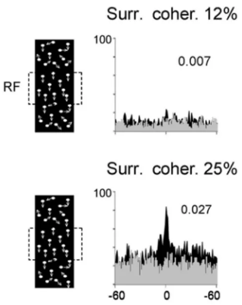
Figure 1. Two examples of cross-correlograms produced by random dots stimuli positioned in the surround above and below of the receptive field (RF), both RF (partially superimposed) are delineated by square. Upper, 12% of dots in the surround are moving in the same direction as dots within the receptive field. This induces a weak insignificant central peak. Lower, 25% of dots in the surround move in the same direction. This higher proportion induces a robust central peak at 0 ms time lag signifying synchronization. X-axis: ms, Y-axis: number of events. Gray areas cross-correlograms are obtained following shuffling; this procedure shows flat cross-correlograms. Left panels are schematic representation of the stimuli, random dots. Number in inserts: synchronization magnitude computed as in reference 58. located in an ultimate area of convergence, which should be quite large in size to contain the extraordinarily large number of cells required to encode all targets potentially to be shown to the sensory systems. Nevertheless an attempt to localize and identify such neurons (‘’Grandmother cells’’) was performed by Tanaka et al. (15,26) using promising imaging techniques, accompanied with more classical electrophysiological recordings. They report grouping of cells along some quite rudimentary properties such as contours. In the olfactory system any one neuron is a poor predictor of odorant identity (28). These cellular properties seem too basic to allow a subtle discrimination of local characteristics that identify an object. Furthermore close properties often evoke more or less equal firing rates, hence the rate code is ubiquitous and may lead to confusion (29).
2.3. Oscillations for Coding
Oscillatory rhythms of theta, alpha, gamma, frequency ranges are hypothesized to reflect key operations in the brain (memory, perception, etc.). One hypothesis states that a non stimulated brain (brain at rest) exhibits oscillations in large networks of oscillatory neurons. A stimulation is then a perturbation of this oscillatory mode (2, 30, 31). It is assumed then that a strongly stimulated
brain disrupts the rhythm at rest and exhibits periods or epoch of sparser oscillatory synchronization. Instead of relating firing rates as a mean of signalling image properties at the neuronal level, it has been suggested that the rhythm of the evoked discharges could be better suited to signal target characteristics.
In fact it has been proposed that within the gamma range (20-100Hz) a definite frequency may be distinctively associated with some properties. A precise frequency would be the tag identifying a particular feature of an object. Along this line gamma oscillations are also stimulus dependent and are considered to be an ‘’information carrier’’ (32- 43). The examination of gamma activity reveals two gamma components which may subserve two different information-processing functions. Early ‘’evoked’’ gamma oscillations tend to be time-locked to the stimulus and may primarily be an index of attention (44, 45). By contrast, the later induced gamma response tends to be loosely time-locked and serves a context processing and integration function. Others (46) suggested that pyramidal cells with long range connections (ascending, descending, and lateral connections) might operate to achieve synchrony or time coordination between separate sites of receptive field inputs (47-49). Recordings of gamma rhythms from humans scalp have shown that gamma oscillations emerge at or above the psychometric threshold suggesting that these rhythms may be linked to brain processes involved in decision making (39). In addition, synchronized activity has been associated with phase correlation between neuronal oscillations in gamma range. Attended sensory stimuli facilitate gamma synchronization which increases perceptual accuracy and behavioral efficiency (50). Extending this role to neural computation, these authors suggested that there is a selection of neurons contributing to sensory input transmission. It must be emphasized however, that synchrony and induced gamma oscillations are two distinct processes since we can record synchrony without oscillations and vice-versa (51, 52).
2.4. Time correlation code: synchronization
Milner (111) and Malsburg (4) advanced an alternative hypothesis. Neurons sharing sensitivity to similar characteristics exhibit synchronous action potentials allowing coherent perception (5, 12, 53-62). More generally, this proposition implies that neuronal signalling rests on time relationships between spikes fired by different and distant neurons. Synchrony will be the acute situation when action potentials of different neurons occurs simultaneously within a 1ms time-window.
Since synchronization involves the participation of many cells it is assumed that the synchrony creates a coding neural assembly allowing the linkage of a constellation of local features (such as colors, angles, motion, direction, etc.) into one coherent picture. Experimentally, the synchrony is disclosed by a central peak when the evoked spikes of two trains are time cross-correlated (57-60). This central peak occurs within a very brief epoch (1 to 5 ms), which reduces the probability of accidental coincidence. (see example in Figure 1). The
magnitude of the central peak is stimulus dependent, that is, units with spatially separated receptive fields fire synchronously in response to objects sharing common features (for instance light bars moving in the same direction, or having same orientations) but asynchronously in response to two independently moving objects (36). Similar data were reported in many species and other sensory systems (20, 63, 60, 63, 64). Yet there is no reason to postulate that targets moving in opposite directions or dissimilar features are less coherent than targets moving in the same direction or sharing similar features. Therefore, any feature belonging to the same object may lead to synchronized activity. Such coding through synchronized activity has been called a neural distributive system. It has also been called linking fields, or binding assemblies (65). Abeles(13) inspired by Hebb(66) developed a radical new concept that the unit of information transmission in the cortex is a synchronously firing group of neurons (synfire group)(Figure 1).
2.5. Coherent and non coherent stimuli
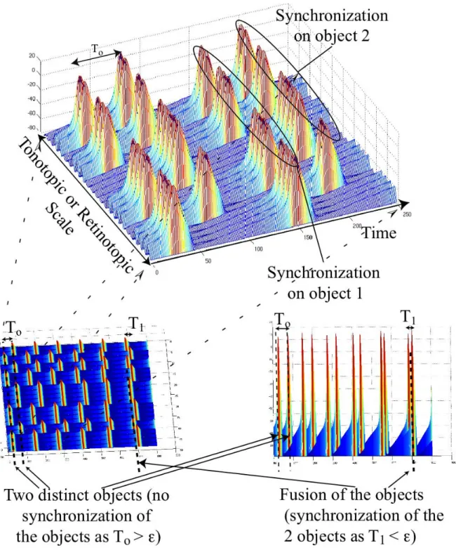
Globally, these neurons will create sparse networks that are superimposed. One neuron can contribute to two neuronal assemblies firing at different intervals or different time lags. These neuronal assemblies of spiking cells implement segmentation and fusion that is the integration of sensory objects’ representation. Although network sparse coding allows signaling of a few trigger features of an object, for instance, a mixture of colors AND orientation. Still it may be insufficient to account for sudden and rapid variations in time and space. Hence, we put forward multilevel sparse networks, or a superposition of neuronal assemblies such as parallel sets of assemblies rather than serial or successive formation of assemblies in a hierarchical stream. The superposition principle or multiplexing allows that several assemblies may be simultaneously active and each member is free to leave one assembly and join another one if the collection of stimuli is modified. Considering that synchrony occurs in the few milliseconds range the formation of several assemblies is rapid, transient and linked to one particular stimulus, and only refractory periods of individual neurons may be a limiting factor. This principle is illustrated in Figure 2. However, under proper conditions any cell may join other sub-networks because the binding is dynamic and changes with time. It should be noted that inputs do not need to be similar but they need to belong to the same object hence applied at the same time.
2.6. Dilemma
There is, however, a conceptual dilemma. In the literature it has been reported that synchrony is mostly induced if visual targets share similar properties such as direction or axis of orientation. Yet, a priori and as mentioned above, there is no reason to postulate that two targets moving in opposite directions are less coherent than targets moving in the same direction. And indeed in support of this latter statement we have shown that images with fractures, orientation disparities or angles induce synchrony (42). Nevertheless, the binding-by-synchrony
hypothesis is flexible and dynamic as cells of an assembly may quit, that is desynchronize, and other neurons may join, that is synchronize, depending on image modifications, thus signifying image properties. In addition synchrony across spike trains operates over large separations between cortical areas.
2.7. Problems with Correlation Hypotheses
In spite of the above-mentioned attractive properties, the correlation hypothesis is not immune from weaknesses (7, 10, 29, 37, 57, 67-73). We shall summarize the most important difficulties. Assuming that synchronization is the vehicle for signalling, then neural populations should be functionally bound together. But are anatomical connectivity and receptive field properties related? How can neurons engage in stimulus induced synchronous interactions with a subset of their inputs when a large percentage of all cell inputs are also active and often spontaneously synchronous? How are synchronization and oscillations computed and read out in the presence of stimuli?
From the above brief review it seems clear that both the serial or hierarchical and the distributive models fall short of explaining the encoding processes of neuronal signals. Therefore more needs to be considered. We show in the following sections that neurons respond to subsets of their inputs. Inside a subset, the activity is synchronous therefore; a neuron receives a time multiplexed subset of activity.
3. SPARSENESS AND MULTIPLEXING
The above brief review calls for supplementary models that may play a role in elucidating the encoding processes carried out by the brain. A body of recent experimental and theoretical data (74) seems to point towards a parallel and distributive organization of neuronal activity.
Although the number of brain neurons is barely imaginable, cells are relatively quite, that is their firing rate is modest (range ~3-5 Hz) (75). It has been suggested that less than 1% of cells are active at any given time (76) because of the high metabolic cost of action potential. Yet one per cent of neurons of a given population are still a fairly large number. The situation is further complicated by the fact that the number of action potentials evoked by the same stimulus varies considerably from trial to trial even though the target is rigorously identical. In addition, two neighbouring cells presumably sharing similar properties react in quite opposite fashion.
3.1. Responses of single cells are variable
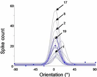
Traditional experiments, in which a microelectrode is implanted in the visual cortex to record single neuron firing evoked by a rather simple stimulus constituted by a dark light edges or a sine-wave grating drifting across the cellular receptive field, reveal that cellular responses vary considerably from one trial to the next, within a time frame of a few seconds. In the example of Figure 3 each curve represents an orientation tuning
Figure 2. Illustration of temporal binding with 24 simulated neurons. In this example, neurons are distributed according to the tonotopic organization of the auditory system. But the same principle holds with a retinotopic organization of vision. Neurons 1,2, 3, 4, 7, 8, 9, 10, 16, 17, 18 and 21, 22 are synchronized and fire at almost the same time, as their input stimulus is dominated mostly by auditory object 1 (102,103). These neurons are bound according to the temporal correlation principle. In this example the other neurons are bound to another auditory object. Segregation of the information is done in the time domain (timing of the neurons) and fusion is performed by the binding (synchronization of the neurons). Second row of the Figure shows how the 24 neurons can dynamically synchronize or desynchronize to segregate two objects or to fuse into one object based on the timing of the neurons. This mechanism allows a rapid change in the binding.To is the time difference between two unsynchronized set of
Figure 3. Responses are unpredictable. Twenty five successive stimulations. Stimulus duration of 4.1 sec. Inter-trial interval 1-3 sec, random. Twenty five tuning curves are shown each fitted with Von Mise’s equation. Although the optimal orientation (0O) remains the same, the
magnitude of the discharges changes considerably in spite of the fact that the stimulus is exactly the same. Number: order of the presentation. X- axis Orientation in degrees, Y- axis firing rate (spike count) Number pointing a few peaks indicate the order of this particular presentation. Magnitude of responses does not change regularly in relationships with the presentation number.
curve as fitted accordingly to Von Mise’s equation (total number of presentation 25).
Although all physical properties of the stimulating sine-wave patch are identical for every presentation, the firing fluctuates considerably regardless of the order of presentation and hence is unpredictable (see Figure 3). This variability between trials is an important issue because the neuronal processing is carried out for every trial as it is unlikely that the receiving neuron average firing rates (as commonly done wit PSTH). A consequence of such variability is that the unit at the next stage receives an input whose strength is variable. Several experimental data support this, for instance the peak of the firing rate is unrelated to the stimulus energy (light intensity in this example). Yen et al., (77) made the stimulus more complex by presenting natural scenes and demonstrated that responses of adjacent neurons in cat striate cortex differ significantly in their peak firing rate when stimulated with natural scenes. The heterogeneity of responses in unanaesthetized monkey suggests that V1 neurons upon stimulation of classical and non classical receptive fields responded in a very selective fashion (78). Such high selectivity in turn augments the sparseness of the population of active neurons. The direct consequence of the above results is that individual neurons carry independent information even when they are situated in the same area such as an orientation column. It may be concluded that individual neurons carry independent information (see below). It must be kept in mind however that averaging responses of many responsive cells produce at population level stable averaged activity. In addition not identical
activity does not necessarily imply that cells are independent of each other. Yet commonly these responses are added with the aim to obtain an averaged firing rate. Since average masks variance specific to each stimuli presentation, averaging prevents coding contained in the event-to-event variances. Nevertheless it has been proposed that this variance is not noise but a signal with encoding values. Furthermore a computation of the response fluctuations suggests that an extremely small proportion of afferent action potential may be associated with the large variance in spite of usually large numbers of afferent axons (79). Yet such processes based on variance do not disqualify encoding through time relationships between spikes. The author postulates then that sparse coding allows for the reduction of number of active fibers (79). Then in order to increase reliability of the signaling, synchrony of action potentials may strengthen the encoding activity, particularly when stimuli contain dissimilar trigger features. This is particularly relevant when evoked discharges have different magnitudes in response to two successive stimuli presentations. It is conceivable, that while neuronal firing may vary the synchrony level may remain rather constant. In addition we have shown that few synchronizing cells are sufficient to increase signaling power (80) ( See below) In spite of a large number of synaptic inputs connecting to a neuron, a small number of synchronized inputs may be sufficient to significantly activate post-synaptic cells. Hence a process that allows increasing the coding potential may be synchronization. The functional gain is that one keeps the number of inputs small but there is an increase of the strength of synaptic transmission.
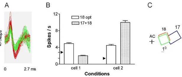
3.2. Modulations of responses of neighboring cells The spike sorting methodology offers substantial advantages when recording neuronal activities. Indeed this technique is based on the ability of the recording system to capture action potentials from a small area and then sort out individual spikes. In general, spikes generated within a 50-100 microns radius may be collected reliably (81). Hence several cells that are close to each other and very often belong to the same functional domain such as same orientation column may be sorted out from the neuronal cluster under the tip of the electrode. In spite of this proximity, neighboring cells display quite different behavior. For instance, Tan et al., (82) showed that two neighboring cells of area 17 of cats sharing the same preferred orientation exhibited opposite response modulation when a remote target was added outside the classical receptive field. One cell reacted with an increased firing rate while the companion cell discharged at a lower rate. (See Figure 4)
Additional investigations have disclosed that adjacent cells display heterogeneous selectivity to spatial frequencies, for instance a low pass cell is adjoining a band pass cell (83, 84). Such disparate distributions of neurons with different sensitivities are quite common in polysensory areas where different sensory modalities converge on single cells. The neuronal reactions are even less homogeneous amongst units belonging to small clusters. The above survey points to a rather small
Figure 4. Neighbouring cells behave differently. Two neurons are sorted out from the same tip of the recording electrode positioned in area 18 of the cat. Cells are color coded (red and green), respective receptive fields are shown in C. Both units have similar optimal orientation. If an additional target is positioned in the receptive field of the cell in area 17, as shown in C, the cell 1 (red) diminishes its firing rate, while the companion unit (green) augments its firing rate. The modulation of responses is shown in B: receptive fields in area 18 are stimulated in isolation, optimal parameters: orientation of sine-wave gratings (opt). 17+18 both cells are simultaneously stimulated by separate sine-wave patches. AC: area centralis. This figure shows that although both cells share orientation domain and are located in very close proximity they react in opposite fashion when additional target is introduced in the visual field. Modified with permission after Tan et al., 2004.
subpopulation of neurons within a limited cortical area that are active during a determined time window.
Similar mixed properties within a small cluster of cells were reported for other sensory modalities. For instance, in the olfactory system it has been demonstrated that both Kenyon cells and the neural circuitry interconnecting the antennal lobe and the mushroom bodies favor the detection of synchronized spatial–temporal patterns that are induced in the antennal lobe. This would allow the tuning of the code for odor identity (74, 85, 86). Therefore, it seems that it is the interactions among neurons in brain circuits that underlie odor perception in the locust. In the auditory system cortico-cortical fibers connect cell groups with large difference in characteristic frequencies, sometimes over one octave and non-overlapping receptive fields. Such heterotopic interconnections allow binding highly composite sounds stretching over large frequency spectrum (87).
The above observations do not exclude the well confirmed classical columnar and modular organizations that are characterized by classes of neurons responding to similar properties of sensory inputs. In spite of that, the modular organization does not rule out the fact that only a small proportion of cells within a column or a cluster may be simultaneously active at any moment and furthermore the neighboring unit may behave in a different fashion due to local interneuronal interactions. In support of the above statement in vivo two-photon calcium imaging demonstrates sparse patterns of correlated activity. In particular there is little dependence. It is suggested the existence of small clustered or intermingled subnetworks within few cells are co-active (88) Furthermore adjacent sub networks may have distinct preference identity. The
dissimilar activity between neighboring cells may be attributed to several organized overlaying maps in the same region such as fine-scale retinotopy, ocular dominance, spatial frequency. Such parcellation leads to sparseness concept.
3.3. Sparseness
Up to this point we have expressed the view that individual neurons fire with a different rate to identical stimuli, or to different properties even though they belong to a single functional domain. We have also described that nearby units behave electrophysiologically in a different fashion. In addition within any given time window (relatively short) cellular activity is low even after stimulus application and the number of active cells is small. In addition it has been suggested by many that the firing rate of a neuron is a poor predictor of the property of the applied stimulus. This pusillanimity of activity introduces the concept of sparse coding (73, 78, 89-92). One must distinguish sparseness of the response of a neuron to some features of a stimulus from sparseness of a functional neuronal network. Therefore there are two distinct definitions of sparseness. The “lifetime sparseness” refers to the variability in the response of a single neuron for instance when a succession of frames of natural images that make up a movie are projected to the visual system. This aspect has been dealt with earlier. The “population sparseness” is defined as the response variability within a population of neurons for each single frame that is presented (89). This second level of analysis shall be discussed and illustrated below. We will now turn to the theme of examining the time relationships between action potentials emitted by two (or more) neurons that may be located at various distances.
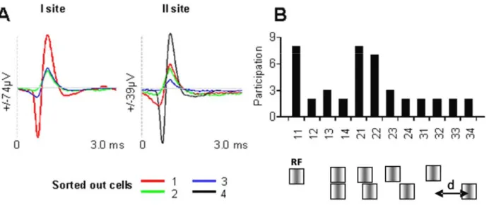
Figure 5. Synchronization is selective to image properties. In A, action potentials are sorted out from two sites in the visual cortex (distance ~400 microns). Three cells in site I and four cells in site II. Cells are color coded. The image (see in B under histogram) is constituted by two identical sine-wave patches (spatial and temporal frequencies, velocity and direction optimized to evoke strongest response from the compound receptive field). The lower patch is displaced laterally in steps. Hence, the parameter that distinguishes images is the distance –d- separating both patches (0.5, 1, 2, 4, 8, 12 deg., center to center). Total number of configurations applied randomly: nine, compound receptive field stimulated in isolation, patches aligned, peripheral patch alone without the central patch (only five configurations are displayed in B, lower row). In B, after shuffling, synchronizations are computed between pairs of cells, pairs are identified by numbers on abscissa. Participation indicates the number of images producing significant level of synchrony (Z score > 4), for instance pair 1-1 synchronized for most stimuli (8/9), whereas synchronization between cells 1 and 2 was quite selective since only two image configurations evoked significant synchrony.
Few neurons have the same selective receptive field, as suggested above, sensory information is represented by a relatively small number of simultaneously active neurons out of a large population. Such sparseness of neuronal activity may seem counterintuitive considering brain imaging data where whole cortical areas are activated by a given stimulus. However, one has to bear in mind that most imaging techniques are indirect, that is, based on hemodynamic changes rather than neural activity. Moreover, those techniques reflect mostly synaptic (neuronal computation) and inhibitory activity is seldom dissociated from excitatory activity (93). On the other hand, sparseness is somewhat instinctive to electrophysiologists, since one can lower an electrode in the cortex without detecting any stimulus-responsive cell (within the limits of the tested stimulus features range). Even when using multiple electrodes the number of active neurons remains small in relation to the cell population sitting under the electrode’s tip.
3.4. Sparseness in the coherent firing: Time relationships between action potentials
We will now focus on the time correlation hypothesis. A previous study (80) measured the level of synchrony between two populations of cells and compared the magnitude of synchrony in relation to image structure (Figure 5).
Two sine-wave patches are applied in the visual fields. A central patch covered both receptive
fields of two pools of cells while a second peripheral patch had a variable distance from the central patch. Hence only the distance between both targets was the characteristic that differentiates various presented images while other properties (size, contrast drift speed and spatial frequency) remained unchanged. In total nine configurations were tested (see legend).
The histogram of Figure 5 indicates the frequency at which time correlations performed between cells recorded in both sites (three cells in site I and four cells in site II) produce significant synchrony. The twelve pairs are identified by numbers labeled in X axis of the histogram of the Figure 5 B. This distribution shows that only pairs 1-1, 2-1, 2-2 exhibited significant synchrony for most (8/8 and 7/9) conditions (SI> 0.012), whereas the remaining pairs synchronized significantly only for a small number of configurations of the image applied to the visual field. This distribution suggests that neuronal assemblies formed by synchrony are rather selective (94). The above results point towards one considerable advantage not shared by other models. Since one assembly is formed for one particular stimulus configuration or set of stimuli, it allows achieving a high degree of selectivity which in turn precludes ubiquitous situations in which several trigger features evoke comparable responses from single neuron. The versatility of neuronal assembly is further discussed in the next Figures.
Figure 6. Synchrony index (SI) measured in relation to orientation differences between two groups of cells. Orientation is indicated in degrees on the X axis. The closer the orientation, the higher the synchrony index (SEM: standard error of the mean).
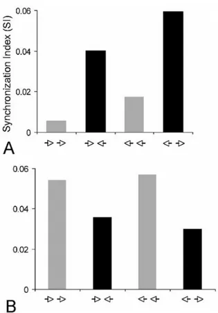
Figure 7. Synchrony depends on the direction of motion. Two sine-wave patches are positioned in respective non-overlapping receptive field. Each sine-wave patch evokes the optimal responses from cells. In A opposite motions (collision or divergent directions) produce higher synchrony indexes than parallel motions. In B the opposite is shown. X-axis: arrow heads motion direction; Y-axis: synchronization index
In Figure (Figure 6) we show that the synchrony magnitude is increased as the orientation difference between two cells becomes narrower. Conversely the wider the difference the smaller the synchrony index between the
two cells. Comparable results were reported elsewhere (7, 37, 55). This result suggests that similar features lead to more frequent action potential coincidence, providing thus a substrate for the formation of encoding assemblies by synchrony. On the other hand such data hinder strong synchronization when features are dissimilar yet belonging to the same image such as targets including cross orientation features of a picture frame. Yet as mentioned previously there is no reason to postulate that disparate targets are less perceptually coherent, for instance parallel motion in opposite direction. Others have suggested that synchrony may potentiate collinear contour synthesis because cells may synchronize within and across different orientation columns (95 )
In next Figure (Figure 7) we illustrate data showing that some pairs synchronize better for parallel motion while another pair exhibits more robust synchrony if gratings are drifting in the opposite direction. The example of Figure 7 compares synchrony levels when drifting directions of two sine-wave patches are in opposite direction (collision or divergent motions) with parallel motions. In A the synchrony index is of higher magnitude for opposite direction whereas when the same stimuli move in the same direction (right or left) the synchrony index is much weaker. In B another pair shows the opposite pattern, that is, parallel motion induces a better synchrony. Altogether, these results suggest that it is possible to achieve synchrony for many characteristics of applied images. Thus, it is unnecessary to call upon a coherency to establish a coding assembly by synchrony. It is worth underscoring that in many of the above studies the firing rate does not change while synchrony magnitudes follow image modifications.
The consequent formation of such assembly is that a few synchronizing cells may suffice to encode one particular target which in turn lead to the sparseness concept because a relatively small number of units are simultaneously committed to encoding a selected number of optimal trigger features. The sparseness or superposition/multiplexing organizations are two notions that complement each other.
Duret et al., computed the coefficient of determination and compared the synchrony degree between single pairs and multiunit recordings from which individual cells were sorted out (80). The study showed that correlating pair wise the neuronal impulses of single cells may produce a synchrony whose magnitude equals the synchrony level produced by correlating multiunit recordings that comprise a much larger number of cells (including the two tested cells initially) and evoke a much higher rate of excitation. These results suggest that for some configurations two synchronizing neurons suffice to signal reliably a target. Such a small number of cells is compatible with the desired scaling-down of neurons involved in brain functions. At population level, cells expressing weaker correlations are contributing to encoding but likely with smaller weight. However, apart from theoretical and computational considerations, the theory of sparse coding is based primarily on two observations:
neural silence, and the cost of cortical computation. Neural silence refers to the fact that neurons fire action potentials rarely or only to very specific stimuli (99). Many investigators reported that recordings in various parts of the cortex detect substantially less neurons than expected on anatomical grounds (100, 101). In the auditory system Eggermont showed that within a cortical column neurons fire synchronously on average about 6 % of their spikes in a 1ms bin (20, 87). Yet such small proportion of time correlated activity is sufficient for cortical reorganization following experimental manipulation (89). This conclusion is further supported by Petersen et al., (102). Analyzing time relationships between spikes, they suggested that small number of neuron is able to support the sensory processing supporting complex whisker-dependent behaviors. To summarize, it appears that at the single cell level the variance of excitability of neurons to identical stimuli poses the risk of ambiguous encoding while the large variations responses modulation of neighboring cells indicate that a neuron, even when belonging to the same functional domain, operates in a relatively independent fashion. This last assertion does not rule out cross influences between neurons belonging to local networks. Yet, coding stimuli features through an assembly of cells that synchronize their action potentials offers the advantage of signaling specific features with less ambiguity. The uncertainty is reduced because only cells excited by specific features are active and in addition the assembly is structured by the time relationships of the respective neurons that lead to perception. Cells lacking such time relationships lose their transient participation in the coding assembly. This in turn, further reduces the number of units belonging to a putative encoding group and hence the noise is further diminished. Finally, since the time relationships, such as synchrony, arise in a very short time window sometime within 1 ms, the establishment and destruction of such an assembly is rapid and it also allows the creation of several multiplexed assemblies, that is, a superposition of several coding assembly allowing flexibility in the representation of several stimuli present in the subject’s sensory space.
3.5. Conventional sparseness measures
In previous section we defined sparseness which implies that few active neurons should enable reliably coding of stimulus. Now we introduce some measures that are used to evaluated the degree of sparseness in a neuronal network. Let us assume that a population of N neurons has sparse activity which is to be measured (as we are interested in comparing the sparse activity between networks). We designate by
r
i the electrical activity of a particular neuroni
from the considered population. One common sparseness measure for a population ofN
neurons is theL
α norm (sometimes called theL
p norm):|| r ||
α=
i=1 N∑
r
iα
1 αwhere
|| .||
α denotes the norm andα
is less than1
when looking for sparse activity in a network ofN
neurons.r
i is the activity of neuroni
(firing rate, firing rate minus the spontaneous firing rate, etc.). The smaller the value ofL
α norm, the greater the sparseness. Kurtosis is another measure of sparseness. The normalized Kurtosis (i.e., Kurtosis excess) is defined as follows3
]
])
[
[(
=
4 4−
−
σ
i ir
r
K
E
E
(1)where
E
[]
is the statistical average of variabler
i andσ
is the standard deviation.K
equals 0 for any Gaussian distribution. It is commonly used to evaluate sparseness as it characterizes the shape of the statistical distribution. For instance if K > 0 the distribution is said to be super-Gaussian (peaked shape); if K < 0 the distribution is sub-Gaussian (flat shape). This definition of flat or peaked shape is relative to the Gaussian distribution where K = 0. The greater the K, the sparser the distribution (the histogram of the distribution exhibits smaller frequencies for the greatestr
i values).Another measure, used by Treves and Rolls (99), is more appropriate to neural data analysis. It is the ratio between the squared statistical average and the variance:
]
[
])
[
(
=
2 2 i ir
r
a
E
E
(2)One estimator of this measure is
ˆ
a =
1
N
i=1 N∑
r
i
21
N
i=1 N∑
r
i2A small value of
a
characterizes sparse activity in the network (if the variance is large compared to the squared mean, then neurons have a different behavior for different stimuli).r
i can be the firing rate andN
the number of neurons in the network.The above measures are used by researchers to understand or to model sparse neuronal activity (or sparse organizations in the brain). In most of these studies the key variable is the firing rate of neurons (or averaged firing rate of groups of neurons). It is known that the timing relationships between spikes in some areas of the brain is
also crucial to encode information (see previous sections). Therefore, we propose that sparseness should also be examined in the context of synchrony between action potentials of pairs of neurons (or even between populations of neurons). In this new context, the sparseness computations described previously are still valid but instead of using the firing rates
r
i we suggest the use of a synchrony magnitude (or synchronization factor)s
i,j between neurons. Depending on the nature of the synchronization the indexi,
j
designates a pair of neurons or two groups of neurons. For instance, the Rolls and Tovee (99) estimator becomes]
[
])
[
(
=
2 , 2 , j i j i syncs
s
a
E
E
(3)A small value of
a
sync indicates that only a few pairs of neurons (or groups of neurons) are synchronized at a specific timet
while a high value shows that most pairs are in synchrony at timet
. For a smalla
sync the probability that different pairs of neurons are synchronized is low. For a greatera
sync, the probability that groups of neurons fire at the same time is greater.3. THE SUPERPOSITION MOSAIC PRINCIPLE: SPARSNESS, SYNCHRONIZATION AND BINDING We introduce in next sections our view towards a more complete model of the superposition principle based on sparse synchronization. Also, means to create a sparse neuronal representation with synchronization is explained below.
4.1. Synchrony for a sparse representation
At initial stages extraction is performed by the peripheral organs of the sensory systems. Coding locations or broad band-pass frequencies are possible at this first stage of the processing. For example, retinotopic organization in the visual system allows placing objects in an appropriate retinal register. The retinotopy is then conveyed to higher levels. For sound frequencies, tonotopic organization in the auditory system begins at the basilar membrane of the cochlea. However, at these peripheral levels of processing the neural activity is not very sparse as many neurons respond to various applied sensory targets with variable strengths since tuning curves may be relatively broad. Also, the coding is likely to be mostly based on the firing rate of neurons.
Then, after 3 to 4 synapses upstream (from the peripheral organs), neurons fire more sparsely with more independent responses. The relative decline of neuronal activity may be attributed to recipical lateral inhibition between parallel ascending streams. As an example, in the Inferior Colliculus the neural responses are relatively well
correlated with the auditory stimuli while in the auditory cortex responses are more sparse and neurons may fire in response to complex sounds (100) . Interestingly, Bruno and Sakmann (101) have shown in rats that thalamocortical synapses have low efficacy as one action potential yields a very weak post-synaptic response. They also have shown that convergent inputs are numerous and synchronous. Hence cortical cells are driven by weak but synchronously active thalamocortical synapses. Their work suggests that, at this level of the brain, synchronization is a key aspect of the information processing. A large number of output neurons can elicit a strong post-synaptic response only if their afferents are conveying action potentials in synchrony. Then the inputs are highly correlated while the outputs are more independent.
Since synchrony of activity between neurons is related to stimulus properties, it seems logical to postulate that such binding by synchrony is less than ubiquitus. Indeed, only cells that are excited by specific features can potentially synchronize. The formation of such a neuronal assembly is specific to specific combinations of properties. As a consequence the feature extraction is facilitated. Figure 8 is a schematic representation of a hypothetic transformation from periphery to the central nervous system with a change in the coding scheme. We assume that at the peripheral level a place topological coding occurs while at the central system a sparsely synchronized coding is dominant. The set of
M
neurons can be dynamically divided into subsets. These subsets are comprised of neurons that are bound via synchrony.Vinje and Gallant (78) have shown the existence of sparseness in the brain. Willmore and Tolhurst (103), Waydo et al. (104) and other authors have suggested that sparsness is a characteristic of the brain and describe its measure.
4.2. Sparse synchronization of oscillatory neuron As discussed in the first section of this paper, oscillatory rhythms in the ranges of theta, alpha, gamma, frequencies are hypothesized to reflect key operations in the brain (memory, perception, etc.). One hypothesis states that a non stimulated brain (i.e. brain at rest) exhibits oscillations in large networks of neurons. A stimulation leads to an alteration of this oscillatory mode (29). It may then be assumed that a strongly stimulated brain disrupts the rhythm at rest (2) and we hypothesize in this paper that brain exhibits periods or epochs of sparser oscillatory synchronization.
5. A MODEL OF SPIKING NEURONAL NETWORK FOR BINDING WITH A POTENTIAL FOR SPARSE SYNCHRONIZATION CODING
In this section, we present a model of a network of spiking neurons that can be used to build a simulated binding neural network based on the superposition principle.
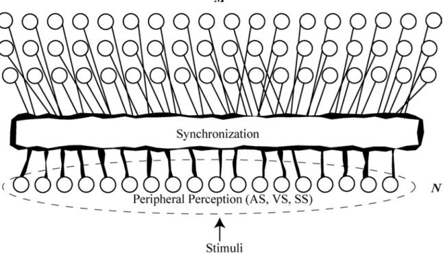
Figure 8. General architecture: illustration of the basic concept of sparsely synchronized activity. The peripheral sensory organ, i.e., retina (VS), cochlea (A.S), or skin (S.S.) uses a nonsparse representation of stimuli (place coding) encoded with
N
neurons (layerN
). This representation is then transformed into a sparsely synchronized representation at higher levels of the brain withM
neurons (whereM
is much higher thanN
). The transformation requires synchronization of the inputs to elicit a response of a small subset of theM
neurons. The peripheral encoding is based on place coding; it is nonsparse and the respective activity of eachN
individual neuron is strongly correlated with the otherN
neurons. On the other hand the activity of eachM
output neuron is weakly correlated with the otherM
neurons. Furthermore, theM
neurons are sparsely synchronized. 5.1. Formal Model of an Isolated NeuronIt is possible to derive general equations that account for cellular responses from which transient and sustained responses can be further investigated in order to integrate the above proposals into a general model. The neuron model we use is the conventional simplistic integrate and fire neuron. Real neurons are much more complex with a richer dynamic. But the integrate and fire spiking neuron can reproduce some of the characteristics of subsets of real neurons. Therefore, there is a great probability that the proposed model behavior can be observed in brains. The sub-threshold potential
v
(t
)
of a simplified integrate and fire neuron with a constant input is:dv(t)
dt
=
−
1
τ
v(t)
+
1
C
I
0 (4))
(t
v
is the output electrical potential,I
o is the input current. Whenv
(t
)
crosses, at timet
spike, a predetermined thresholdθ
, the neuron fires and emits a spikeAP(t
spike)
. Thenv
(t
)
is reset toV
o. C is the membrane capacitance,τ
has the dimension of a timeconstant expressed in seconds. After integration, the final expression of
v
(t
)
is)
(1
=
)
(
τ t oe
C
I
t
v
−
− (5)and we assume that the initial instant
t
o is equal to 0. The neuron that is described by equation (5) can oscillate. When the membrane potentialv
(t
)
of a neuron)
,
( j
i
becomes, at timet
spike, equal or greater than the internal thresholdθ
, the neuron shall fire generating a spike:θ
δ
(
−
)
(
)
≥
*
)
(
=
)
;
,
(
i
j
t
spiket
t
t
spikeif
v
t
spikex
AP
(6)otherwise
x
(
i
,
j
;
t
)
=
0
. After firing, the membrane potentialv
(
t
spike+)
is reset toV
o.AP
(t
)
is the action potential (usually assumed to be equal to0
whent
<
0
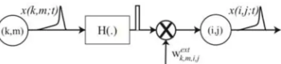
Figure 9. Details of a connection from neuron
( m
k
,
)
projecting into neuron( j
i
,
)
in another layer. The initial action potentialAP
(
t
spike)
is squared by theH
(.)
transform and then multiplied with weightw
. This simplifies the simulation while preserving the aptitude of the neural network to perform binding by synchronization.and having an impulsive waveform with a finite duration), * is the convolution,
δ
(t
)
is the Dirac impulsion1 function andt
spike+=
lim
ε→0
(t
spike+
ε)
(8) The above relations express the rhythmic behavior of a single cell. In fact, ifC
I
oin equation 5 is greater or equal to
θ
then the neuron can oscillate even if the neurons it is connected to are not active2. The phase and the frequency of the oscillations will depend on the activity of cells to which it is connected. On the other hand ifC
I
ois smaller than the internal threshold
θ
then, to fire the neuron has to be part of a network3 .5.2. The neuron inside a neural network
Now, let us consider neurons that are connected to other cells. We use two types of connections: local for neurons inside the same layer and global connections between neurons being in different layers. An example of this is given on Figure 13. Also, instead of manipulating action potentials the model is built around impulses as illustrated in Figure 9.
For an example, Figure 13 illustrates the connectivity pattern between a neuron
( j
i
,
)
and 3 neurons( m
k
,
)
. One neuron( m
k
,
)
is on the same layer and the two other neurons( m
k
,
)
are located on other layers. Connections are bi-directional.
5.3. Contribution from the other neurons
Connecting neurons together and writing the general equation that describes the network behavior is our next aim. Let us assume that a neuron
( j
i
,
)
is connected to other neurons and that it receives a total contribution)
(
,
t
S
i j from the other neurons it is connected to (neuronsint
m
k
,
)
(
from the same layer, neurons(
k
,
m
)
ext from the other layers, and inhibition - crudely modeled here as a global inhibitor. We use, as a notation, the cardinal position of a neuron in the layer plane. Neuron( j
i
,
)
is located inrow
i
and columnj
, and neuron( m
k
,
)
may be any neuron connected to neuron( j
i
,
)
in the same or in another layer. At some time t, the contributionS
i,j(
t
)
from all neurons in the neural network to neuron( j
i
,
)
is{
}
{
}
∑
∑
∈ ∈−
+
=
) , ( , int int , , , ) , ( , , , , , int)
(
))
;
,
(
(
))
;
,
(
(
)
(
j i N m k m k j i j i N m k ext ext m k j i j it
G
t
m
k
x
H
w
t
m
k
x
H
w
t
S
estη
(9) where ext m k j iw
, , , are the connecting weights between neuron)
,
( j
i
and neurons( m
k
,
)
, with neuron( j
i
,
)
and neurons( m
k
,
)
being in a different layer.int m k j i
w
, , , are the connecting weights between neuron( j
i
,
)
and neurons)
,
( m
k
inside the same layer.H
(.)
is the function whereH(x(k,m;t))
equals1
if and only ifx(k,m;t) > 0
.x(k,m;t)
is the spike output from neurons( m
k
,
)
. Thefirst term in the right-hand side of equation (9) is the total contribution coming from all neurons in external layers; the second term is the total contribution coming from all neurons in the same layer as neuron
( j
i
,
)
, and the last term is the contribution from the global inhibitor.The inhibitory influences are integrated into one global inhibitory controller
η
G
(t
)
.η
is a constant that weights the global inhibitor controller contribution. We assume that this inhibitor is connected to all neurons. Its membrane potentialu
(t
)
follows the equation:σ
ζ
+
−
(
)
=
)
(
t
u
dt
t
du
(10)It is a leaky integrator that is leading (
σ
=
1
) only if the global activity of the network is higher than a predefined thresholdΘ
, otherwiseσ
=
0
in equation 104. The final expression for a neuron( j
i
,
)
inside the network becomesC
dt
τ
τ
,C
are the same variables as in equation 5,I
o is the external input to the neuron (for example: stimulus) and)
(
,
t
S
i j is the total contribution coming from the other neurons of the network as given in equation 9.5.4. Expressing the connection weights
The synaptic weight depends on the similarity between features. That is, the closer the features, the stronger the synaptic weights should be. Conversely, neurons characterizing dissimilar features should exert a weak influence and should have small synaptic weights. This is in accordance with the Hebbian learning rule. Although the Hebbian learning rule yields equilibrium and stabilization of the synaptic weights through self-organization of the network, it requires time. We bypass this step by setting up the weights depending on the stimulus inputs (equation 13). In principle this procedure is faster than using the Hebbian rule. Another advantage of this approach is that the designer can encode the network behaviors into the weights. It is then possible to assign strong weights between two visual features of targets moving in opposite directions.
The connecting weights have the general form:
wi, j,k ,mint =
wmaxint
Card{Nint(i, j)}⋅e −λ|ii,j(t)−ik,m(t)|
for intra− layer connections
(13)
wi, j,k ,m
ext = wmaxext
Card{Next(i, j)}⋅ e
−λ|ii, j (t)−ik,m(t)|
for extra− layer connections
w
i, j,k,mint
are connections inside the same layer.
w
i, j,k,mext are connections between two different layers (neurons)
,
( j
i
and( m
k
,
)
do not belong to the same layer).ext max
w
,w
maxint andCard{N
int(i, j)}
,Card{N
ext(i, j)}
are normalization factors.)| ; , ( ) ; , ( |pijt pkmt
e
−λ −can be interpreted as a measure of the difference between inputs of neurons
( j
i
,
)
and( m
k
,
)
, i.e., the difference between local properties of trigger features that activate both cells. For instance it may be two orientations characterizing the same image. Herei
i,j(
t
)
andi
k,m(
t
)
are respectively external inputs to)
,
( j
i
neuron
andneuron(k,m)
.neuron(k,m)
is physically connected with neuron
neuron
( j
i
,
)
. One definesN
ext( j
i
,
)
as the set of neurons connected to neuron( j
i
,
)
that are not on the same layer as neuron)
,
( j
i
.N
int( j
i
,
)
is the set of neurons connected to neuron( j
i
,
)
that are on the same layer as neuron( j
i
,
)
.)}
,
(
{
N
i
j
Card
is equal to the cardinal number (number of elements) of the setN
( j
i
,
)
containing allor different layers). Therefore,
)}
,
(
)
,
(
{
=
)}
,
(
{
N
i
j
Card
N
i
j
N
i
j
Card
ext∪
int.
In summary, we have presented and implemented a model that is used to illustrate next sections and our superposition principe.
6 . OBJECTS REPRESENTATIONS
We first describe how sub-populations of neurons that are binded with synchronization remain synchronized even if they are affine transformed of each others. To ease the understanding we illustrate the principle on images where features are based on image pixel’s structures. It must be kept in mind that, in the brain, much more complex features are binded all-together. The proposed synchrony model refers to a potential central processing and not to peripheral. Second, we present our affine superposition model principle as a potential representation of objects in the brain. Again, illustrations of our model are given for visual stimuli, but the same principle applies to auditory and other sensory stimuli.
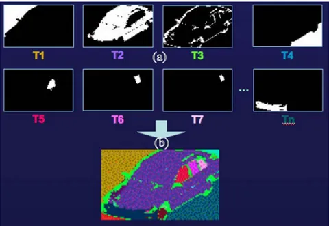
6.1. Feature Extractions: Illustration with Image An object may be represented by a set of active neurons (points) corresponding to appropriate trigger features exciting responsive neurons. This principle is illustrated in Figure 10. Eight responsive neurons (written as
T1,T2,...,T8
) are selectively sensitive to eight features belonging to an image of a car. Each responsive neuron fires only if its inputs are synchronized. Coming back to Figure 8, these neurons could fit in layer M with distinctive receptive fields being obtained from the synchronization of a great number of neurons in layer N.In Figure 10, the synchronized inputs to each respective