HAL Id: tel-02266365
https://pastel.archives-ouvertes.fr/tel-02266365
Submitted on 14 Aug 2019
HAL is a multi-disciplinary open access
archive for the deposit and dissemination of sci-entific research documents, whether they are pub-lished or not. The documents may come from teaching and research institutions in France or abroad, or from public or private research centers.
L’archive ouverte pluridisciplinaire HAL, est destinée au dépôt et à la diffusion de documents scientifiques de niveau recherche, publiés ou non, émanant des établissements d’enseignement et de recherche français ou étrangers, des laboratoires publics ou privés.
statistical estimation inhigh dimension
Mohamed Ndaoud
To cite this version:
Mohamed Ndaoud. Contributions to variable selection, clustering and statistical estimation inhigh dimension. Statistics [math.ST]. Université Paris-Saclay, 2019. English. �NNT : 2019SACLG005�. �tel-02266365�
Th
`ese
de
doctor
at
NNT
:2019SA
CLG005
Contributions to variable selection,
clustering and statistical estimation in
high dimension
Th`ese de doctorat de l’Universit´e Paris-Saclay pr´epar´ee `a l’ ´Ecole nationale de la statistique et de l’administration ´economique ´Ecole doctorale no574- ´Ecole doctorale de math´ematiques Hadamard (EDMH)Sp´ecialit´e de doctorat : Math´ematiques Fondamentales
Th`ese pr´esent´ee et soutenue `a Palaiseau, le 03 Juillet 2019, par
M
OHAMEDN
DAOUDComposition du Jury : Alexandre Tsybakov
ENSAE Paris Directeur de th`ese Alexandra Carpentier
Magdeburg University Rapporteuse Yihong Wu
Yale University Rapporteur Cristina Butucea
ENSAE Paris Examinatrice
Christophe Giraud
Universit´e Paris-Sud Pr´esident du jury Enno Mammen
Heidelberg University Examinateur Nicolas Verzelen
Beyond the mountains, more mountains. Haitian Proverb
À mes parents, mes deux sœurs
et Raouia
Remerciements
Mes premières pensées vont droit à Sacha, mon directeur de thèse. Je tiens à te remercier pour m’avoir encadré, pour m’avoir fait confiance mais surtout pour m’avoir converti. Jeune étudiant hésitant à pousser les portes du monde de la finance, tu as su me donner une chance, et ainsi un nouveau départ, sans vraiment te poser de questions quant à ma formation. Ce geste en dit beaucoup sur ta personne ainsi que ta noble vocation à former la prochaine génération de chercheurs. Ta patience, ta générosité, ta rigueur ainsi que tous les échanges qu’on a eus me marqueront à jamais. Je suis certain que notre collaboration ne s’arrêtera pas après ma soutenance.
Alexandra et Yihong m’ont fait l’immense honneur d’accepter de rapporter cette thèse. Je leur suis très reconnaissant. Je ne saurais assez les remercier. Mes remer-ciements vont ensuite au jury de thèse. Cristina, pour avoir été un exemple de pro-fessionnalisme pendant nos quelques collaborations. Je suis ravi de faire partie de tes coauteurs. Christophe, pour avoir été l’un des premiers à m’encourager à faire de la recherche. Merci pour tes précieux conseils tout au long de mon parcours ainsi que pour m’avoir recommandé chaque fois que j’en avais besoin. Ton livre m’a été d’une grande aide pendant ces trois ans. Enno, pour ton invitation à Heidelberg et notre collabora-tion en cours. Je suis très honoré de pouvoir apprendre à tes côtés. Nicolas, pour tes nombreux travaux qui ont inspiré plusieurs résultats de cette thèse.
Une pensée particulière est pour mes autres collaborateurs Laëtitia, Natalia et Olivier. J’ai beaucoup profité de travailler avec vous. Je suis très fier d’avoir pu progresser à vos côtés et des résultats que nous avons obtenus ensemble.
Ce fut un réel plaisir d’effectuer ma thèse au département de statistiques de l’ENSAE. Je n’oublierais jamais tous les moments conviviaux passés ensemble, nos pauses café ainsi que nos matchs de foot. Je suis heureux d’y avoir rencontré des collègues que je considère aujourd’hui mes amis, voire ma seconde famille.
Je remercie Arnak pour m’avoir toujours conseillé. Tu es pour moi un chercheur exemplaire sur les deux plans humain ainsi que scientifique. Guillaume pour tous nos échanges scientifiques, surtout pendant le déjeuner. Marco, pour ta gentillesse et nos séances de musculation. Pierre pour avoir été une personne sur qui j’ai pu compter pen-dant ces trois années. J’espère que notre amitié va durer longtemps. Victor-Emmanuel pour ta bonne humeur. Nos discussions m’ont souvent égayé. J’espère qu’on pourra travailler ensemble un jour.
Ensuite mes remerciements vont droit à mes cobureaux: Gautier et Geoffrey, à mon colocataire et compagnon de thèse Lionel, ainsi qu’à mes coéquipiers de foot: Badr, Monsour, Wasfe, Aurélien et Arshak. Enfin je remercie: Nicolas, Jérémy, Léna, Solenne, Lucie, Mamadou, Suzanne, Julien, Mehdi, Edwin, Alexander, Philip, Avo, Amir, Christophe, Boris, Alexis, Gabriel et François-Pierre.
Merci à mes parents et mes soeurs pour leur soutien infaillible tout au long de ces trois années. J’espère qu’ils sont fiers de moi. Merci à mes amis proches A., J., I.,R., O. pour tous les moments passés ensemble. Puisse notre amitié durer à jamais.
Contents
Résumé Substantiel 1
1 Introduction 3
1.1 Structured High-Dimensional Models . . . 3
1.2 Interaction with other disciplines . . . 7
1.3 Variable Selection and Clustering . . . 12
2 Overview of the Results 17 2.1 Variable Selection in High-Dimensional Linear Regression . . . 17
2.2 Clustering in Gaussian Mixture Model . . . 21
2.3 Adaptive robust estimation in sparse vector model . . . 23
2.4 Simulation of Gaussian processes . . . 25
I Variable Selection in High-Dimensional Linear Regression
27
3 Variable selection with Hamming loss 29 3.1 Introduction . . . 293.2 Nonasymptotic minimax selectors . . . 32
3.3 Generalizations and extensions . . . 35
3.4 Asymptotic analysis. Phase transitions . . . 39
3.5 Adaptive selectors . . . 44
3.6 Appendix: Main proofs . . . 47
3.7 Appendix: More proofs of lower bounds . . . 60
4 Optimal variable selection and adaptive noisy Compressed Sensing 67 4.1 Introduction . . . 67
4.2 Non-asymptotic bounds on the minimax risk . . . 72
4.3 Phase transition . . . 76
4.4 Nearly optimal adaptive procedures . . . 79
4.5 Generalization to sub-Gaussian distributions . . . 83
4.6 Robustness through MOM thresholding . . . 85
4.7 Conclusion . . . 88
4.8 Appendix: Proofs . . . 88 vii
5 Interplay of minimax estimation and minimax support recovery under
sparsity 97
5.1 Introduction . . . 97
5.2 Towards more optimistic lower bounds for estimation . . . 101
5.3 Optimal scaled minimax estimators . . . 103
5.4 Adaptative scaled minimax estimators . . . 105
5.5 Conclusion . . . 107
5.6 Appendix: Proofs . . . 108
II From Variable Selection to Community Detection
119
6 Sharp optimal recovery in the two component Gaussian Mixture Model121 6.1 Introduction . . . 1216.2 Non-asymptotic fundamental limits in the Gaussian mixture model . . . 126
6.3 Spectral initialization . . . 128
6.4 A rate optimal practical algorithm . . . 130
6.5 Asymptotic analysis. Phase transitions . . . 131
6.6 Discussion and open problems . . . 132
6.7 Asymptotic analysis: almost full recovery . . . 133
6.8 Appendix: Main proofs . . . 135
6.9 Appendix: Technical lemmas . . . 146
III Adaptive robust estimation
149
7 Adaptive robust estimation in sparse vector model 151 7.1 Introduction . . . 1517.2 Estimation of the sparse vector . . . 154
7.3 Estimation of the norm . . . 156
7.4 Estimating the variance of the noise . . . 160
7.5 Appendix: Proofs of the upper bounds . . . 165
7.6 Appendix: Proofs of the lower bounds . . . 175
7.7 Appendix: Technical lemmas . . . 182
IV Simulation of Gaussian processes under stationarity
191
8 Harmonic analysis meets stationarity: A general framework for series expansions of special Gaussian processes 193 8.1 Introduction . . . 1938.2 On harmonic properties of the class Gamma . . . 196
8.3 Constructing the fractional Brownian motion . . . 198
8.4 Generalization to special Gaussian processes . . . 202
8.5 Application: Functional quantization . . . 206
8.6 Conclusion . . . 207
CONTENTS ix
Conclusion 213
Résumé Substantiel
Au cours des dernières décennies, la statistique a été au centre de l’attention, et ce, de bien des façons. Grâce à des améliorations technologiques, par exemple l’augmentation des émissions de la performance des ordinateurs et l’essor du partage de la capacité de données, les statistiques à grande dimension ont été extrêmement dynamiques. En conséquence, ce domaine est devenu l’un des principaux piliers du paysage statistique moderne.
Le cadre statistique standard tient compte du cas où la taille de l’échantillon est rela-tivement grande et que la dimension des observations est beaucoup plus petite. Comme on l’a fait remarquer dans Giraud (2014), l’évolution technologique de l’informatique a poussé à un changement de paradigme de la théorie statistique classique à la statistique de grande dimension. Plus précisément, nous caractérisons un problème statistique comme étant hautement dimensionnel lorsque la dimension des observations est beau-coup plus grande que la taille de l’échantillon. Elle est devenue plus courante avec l’augmentation du nombre de caractéristiques accessibles des données.
D’une manière générale, les problèmes statistiques sont mal posés dans un contexte de grande dimension. D’autres hypothèses sur la structure du modèle sous-jacent sont nécessaires afin de rendre le problème plus important. Par exemple, dans un problème de régression à dimensions élevées, on peut supposer que le vecteur à estimer est parci-monieux (c’est à dire que peu de composantes sont non nulles), ou que la matrice du signal est de faible rang lorsqu’il s’agit d’estimer une matrice. Ces hypothèses sont généralement très réalistes et confirmées par des données empiriques. C’est ce que l’on peut qualifier de statistiques structurées de grande dimension.
Dans cette thèse, nous nous sommes concentrés sur certains problèmes spécifiques aux statistiques de grande dimension et à leurs applications à l’apprentissage automa-tique.
Notre principale contribution porte sur le problème de la sélection de variables dans la régression linéaire à grande dimension. Nous dérivons des limites non-asymptotiques pour le risque minimax de recouvrement du support sous la perte de Hamming en
es-pérance dans le modèle de bruit Gaussien en Rd pour les classes de vecteurs s-sparse
séparés de 0 par une constante a > 0. Dans certains cas, on trouve aussi explicite-ment les sélecteurs minimax correspondants et leurs variantes adaptatives. Comme corollaires, nous caractérisons précisément une transition de phase asymptotique pour le recouvrement presque complet ainsi que le recouvrement exact.
En ce qui concerne le problème de recouvrement du support exact en acquisition comprimée, nous proposons un algorithme de recouvrement du support exact dans le cadre de l’acquisition comprimée bruitée où toutes les entrées de la matrice de com-pression sont des Gaussiennes i.i.d. Notre méthode est la première procédure en temps
polynomial à atteindre les mêmes conditions de recouvrement exact que le décodeur de recherche exhaustive étudié dans Rad (2011) et Wainwright (2009a). Notre procédure a l’avantage d’être adaptative à tous les paramètres du problème, robuste et calculable en temps polynomial.
Motivé par l’interaction entre l’estimation et le recouvrement du support, nous in-troduisons une nouvelle notion de minimaxité pour l’estimation parcimonieuse dans le modèle de régression linéaire à grande dimension. Nous présentons des bornes inférieures plus optimistes que celles données par la théorie classique du minimax et améliorons ainsi les résultats existants. Nous récupérons le résultat précis de Donoho et al. (1992) pour la minimaxité globale à la suite de notre étude. En fixant l’échelle du rapport signal/bruit, nous prouvons que l’erreur d’estimation peut être beaucoup plus petite que l’erreur min-imax globale. Entre autres, nous montrons que le recouvrement exact du support n’est pas nécessaire pour atteindre la meilleure erreur d’estimation.
En ce qui concerne le problème de clustering dans le modèle de mélange Gaussien à deux composantes, nous fournissons une caractérisation non-asymptotique précise du risque minimax de Hamming. En conséquence, nous récupérons la transition de phase précise pour un recouvrement exact dans ce modèle. À savoir, la transition de phase se
produit autour du seuil = ¯n tel que
¯2 n= 2 ✓ 1 + r 1 + 2p n log n ◆ log n.
Notre procédure atteint le seuil précédent. C’est une variante de l’algorithme de Lloyd initialisée par une méthode spectrale. Cette procédure est entièrement adaptative, opti-male en termes de taux et simple en termes de calcul. Il s’avère que notre procédure est, à notre connaissance, la première méthode rapide pour obtenir un recouvrement exact optimal.
Une autre contribution principale est consacrée à certains effets de l’adaptabilité sous l’hypothèse de parcimonie, où l’adaptabilité est soit par rapport au niveau du bruit, soit par rapport à sa loi nominale. Nous dérivons les taux minimax optimaux et présentons
des estimateurs correspondants pour l’estimation de la variance du bruit 2 pour
dif-férentes classes de bruit. Par exemple, lorsque la distribution du bruit est exactement
connue, 2 peut être estimée plus précisément si le bruit a des queues polynomiales
connues plutôt que d’appartenir à la classe de bruit sous-Gaussienne. Des résultats
similaires ont été obtenus pour le problème de l’estimation minimax de k✓k2. Enfin,
nous étudions l’optimalité minimax de l’estimation de ✓ lorsque le bruit appartient à une classe de distributions avec queues polynomiales ou queues exponentielles. Nous calculons les taux minimax pour ces paramètres. Une conclusion inattendue est que dans le modèle à moyenne parcimonieuse, les taux optimaux sont beaucoup plus lents et dépendent de l’indice polynomial du bruit par opposition aux taux en régression avec des régresseurs "bien répartis".
Dans notre dernière contribution, nous proposons une nouvelle approche pour dériver des développements en série pour certains processus Gaussiens basée sur l’analyse har-monique de leur fonction de covariance. En particulier, une nouvelle série simple est dérivée pour le mouvement Brownien fractionnaire. La convergence de cette dernière série se maintient en moyenne quadratique ainsi qu’uniformément presque sûrement, avec un taux optimal de décroissance du reste de la série. Nous développons également un cadre général de séries convergentes pour certaines classes de processus Gaussiens.
Chapter 1
Introduction
The aim of this chapter is to introduce some of the recent topics of interest in high-dimensional statistics, not necessarily related to the results of the thesis. The list of references is not exhaustive and more details are provided in the following chapters. We inform the reader that the notation may change from chapter to chapter.
1.1 Structured High-Dimensional Models
Over the last decades, Statistics has been at the center of attention, in a wide variety of ways. Thanks to technological improvements, for instance the increase of computer performance and the soar of sharing data capacity, high-dimensional statistics has been extremely dynamic. As a consequence, this field became one of the main pillars of the modern statistical landscape.
The standard statistical framework considers the case where the sample size is rel-atively large and the dimension of the observations substantially smaller. As pointed out in Giraud (2014), the technological evolution of computing has urged a shift of paradigm from classical statistical theory to high-dimensional statistics. More precisely, we characterize a statistical problem as high-dimensional whenever the dimension of the observations is much larger than the sample size. It has become more common with the increase of accessible features of data.
Generally speaking, statistical problems are ill posed in the high-dimensional setting. Further assumptions on the structure of the underlying model are required in order to make the problem more significant. For instance in a problem of high-dimensional regression, we may assume that the vector to estimate is sparse (i.e. only few components are non-zero), or that the signal matrix is of small rank when dealing with matrix estimation. These assumptions are usually very realistic and endorsed by empirical evidence. This is what can described as as Structured High-Dimensional Statistics.
A new paradigm
One way to summarize some paradigms of modern Statistics is the following. For statis-tical methods to be "successful", they need to fulfill the OCAR criterion, where OCAR stands respectively for Optimality, Computational tractability, Adaptivity and Robust-ness.
• Optimality
In order to evaluate and compare algorithms the oldest criterion is probably the statistical optimality. An estimator is said to be optimal if it cannot be improved in some sense. A widely used criterion is minimax optimality. The notion of minimax optimality is relative to some risk. In order to make this notion more
transparent, let us assume that we observe i.i.d realizations X1, . . . , Xn of some
random variable X. Suppose moreover that the distribution of X is given by
P✓ for some parameter ✓ 2 ⇥ we are interested in. Given a semi-distance d,
the performance of an estimator ˆ✓n = ˆ✓n(X1, . . . , Xn) of ✓ is measured by the
maximum risk of this estimator on ⇥:
r(ˆ✓n) = sup ✓2⇥ E✓ ⇣ d2(ˆ✓n, ✓) ⌘ ,
where E✓ denotes the expectation with respect to (X1, . . . , Xn). The minimax risk
is given by the smallest worst-case risk reached among all measurable estimators. It is given by:
R⇤n = inf
ˆ ✓n
r(ˆ✓n),
where the infimum is over all estimators. In practice, we have a general framework to derive minimax lower bounds, cf. Tsybakov (2008). We say that an estimator
✓⇤
n is non-asymptotically minimax optimal if the following holds
r(✓⇤n) CR⇤n,
where C > 0 is a constant.
Given this criterion, we are interested in estimators achieving the minimax optimal rate. As an example, consider the problem of low rank matrix estimation. It turns out that a simple spectral procedure is minimax optimal. Indeed, Koltchinskii et al. (2011) gives a lower bound and a matching upper bound for the problem of minimax low-rank matrix estimation through a nuclear norm penalization pro-cedure. We recall that the notion of minimax optimality is one way to define optimality, and one may think of other criteria, for instance a Bayesian risk in-stead of the minimax risk.
We should point out that the notion of minimax risk is not impeccable. In general, this notion is pessimistic since the worst case scenario may be located in a tiny region of ⇥. In that case, the worst-case scenario is not likely to be realized. This fact is detailed further in Chapter 5.
• Computational Tractability
Computational tractability captures whether a given algorithm can be computed in polynomial time. For instance, a method based on a sample of size N that
runs in O(N2) is practical while another one running in O(epN) is not. The
recent importance of this criterion is due to the explosion of sample sizes versus the limited capacity of our actual machines. Indeed, for many statistical problems computational by non-tractable exhaustive search methods (i.e. greedy methods testing all possible solutions in a finite set of an exponential size) are shown to be optimal from a statistical point of view.
1.1. STRUCTURED HIGH-DIMENSIONAL MODELS 5 One of the most challenging problems related to tractability of algorithms is related to computational lower bounds. While a large body of techniques is available to derive general lower bounds for minimax risks, not much in known when we restrict the class of estimators to polynomial time methods. Karp (1972) has proved, for the specific problem of detecting the presence of a hidden clique, that there is a non trivial gap between what could be achieved by any method and by polynomial time methods. This breakthrough shows that it is not always possible to reach statistical optimality through polynomial methods. Inspired by the planted clique problem, the previous fact has been extended to Sparse PCA among many other problems, cf. Berthet and Rigollet (2013). Apart from this reduction to the planted clique problem, it is still unclear how to derive general computational lower bounds having the same flavour as information-theoretical lower bounds. • Adaptivity
In order to measure the performance of a given estimator, we may assume that the data is generated according to some model. This model is used further to evaluate the algorithm. Usually, a model depends on different parameters, and the proposed estimator may depend on these parameters. The criterion of adaptivity aims to compare two optimal algorithms through their ability to adapt to the parameters of the model. Sometimes optimality and adaptive optimality are slightly different but in many scenarios adaptivity is possible at almost no cost. For instance consider the problem of high-dimensional estimation in linear regression. The performance of LASSO and SLOPE (Bogdan et al. (2015)) estimators is studied in Bellec et al. (2018) under similar conditions on the design. It turns out that a sparsity dependent tuning of LASSO achieves the minimax estimation rate. While LASSO requires a prior knowledge of the sparsity, SLOPE is adaptively minimax optimal. Still, we may argue that SLOPE requires a higher complexity due to the sorting step. This may be seen as the price to pay for adaptation. To the best of our knowledge, the question of minimax adaptive optimality using a fixed complexity has not been addressed so far. Generally speaking adaptation to sparsity can be done through two main techniques, either by a Lepski type method or by sorted thresholding procedures as in the Benjamini-Hochberg procedure.
• Robustness
There are two popular notions of robustness. The classical robustness is with respect to outliers, in the sense that a small fraction of data is corrupted by outliers. The Huber contamination model is a typical example of it (Huber (1992)). Let
X1, . . . , Xn be n i.i.d random variables and ¯p the probability distribution of Xi.
There are two probability measures p, q and a real ✏ 2 [0, 1/2) such that ¯
p = (1 ✏)p + ✏q, 8i 2 {1, . . . , n}.
This model corresponds to assuming that (1 ✏)-fraction of observations, called
inliers, are drawn from a reference measure p, whereas ✏-fraction of observations are outliers and are drawn from another distribution q. In general, all the three parameters p, q and ✏ are unknown. The parameter of interest is the reference distribution p, whereas q and ✏ play the role of nuisance parameters. For instance, the particular case where p is the normal distribution with unknown mean ✓ and
variance 1 has been extensively studied in the last decade, cf. Diakonikolas et al. (2016, 2017) and references therein.
In dimension one, it is clear that the empirical median is a robust alternative to the empirical mean. The problem becomes more complicated in higher dimensions since there are many generalizations of median in dimension larger than two. For the normal mean estimation problem, Chen et al. (2018) show that robust estima-tion can be achieved in a minimax sense through Tukey’s median (Tukey (1975)). Unfortunately, this approach is not computationally efficient. Recently, many ef-forts has been made to prove similar results using polynomial time methods, for instance, filtering techniques (Diakonikolas et al. (2016)) and group threshold-ing (Collier and Dalalyan (2017)). We should add here that the outliers may be deterministic, random or even adversarial.
A more recent notion of robustness is with respect to heavy tailed noise. It is pioneered by Catoni (2012). Although the sub-Gaussian noise assumption is not always realistic, it is quite convenient in order to derive non-asymptotic results thanks to concentration properties. These guarantees fail under heavy tail
as-sumptions of the noise. Assume that we observe X1, . . . , Xn2 Rp such that
Xi = µ + ⇠i,
where ⇠i are i.i.d centered sub-Gaussian random vectors with independent entries.
In that case the empirical mean ˆX satisfies, for any given confidence level > 0,
the following: P k ˆX µk C r p n + r log 1/ n !! ,
where C > 0 and k.k denotes the `2 norm. Recently, the Median-Of-Means
esti-mator (Nemirovskii and Yudin (1983)) was shown to achieve similar results under very mild assumptions on the noise in dimension one, cf. Devroye et al. (2016). Generalization to high dimensions through tractable methods has been an active field of research in recent years. The recent paper by Cherapanamjeri et al. (2019), exhibits a new method based on an SDP relaxation achieving similar results in polynomial time. Their algorithm is significantly faster than the one proposed by Hopkins (2018), which was, to the best of our knowledge, the first polynomial method achieving sub-Gaussian guarantees for mean estimation under only the second moment assumption.
To sum up, we have presented some criteria that we believe are in the core of mod-ern Statistics. Following this perspective, the ideal algorithm would satisfy the OCAR. However this is subject to further evolution. Distributional implementation along with storage capacity are already attracting attention, cf. Szabo and van Zanten (2017) and Ding et al. (2019) for recent advances in these directions. If the data keeps grow-ing without improvgrow-ing the speed limitations then at some point distributed algorithms will become to polynomial time methods what today polynomial time methods are for exponential time methods.
1.2. INTERACTION WITH OTHER DISCIPLINES 7
1.2 Interaction with other disciplines
In the previous paragraph, we described what we may consider as the modern statis-tical paradigm. It is also important to recall that modern statistics have been shaped through many interactions with other disciplines. We only investigate here two of these interactions that are of interest in the rest of this manuscript.
Interaction with statistical physics and mechanics
Matter exists in different phases, different states of matter with qualitatively different properties. A phase transition is a singularity in its thermodynamic behavior. As one changes the macroscopic variables of a system, sometimes its properties will abruptly change, often in a dramatic way. We devote this section to discuss some popular phase transitions that has inspired research in Statistics.
Percolation
Among the most popular models involving phase transitions in physics are the Ising model (a model for magnetic solids) and percolation. We only consider here the latter model for simplicity of its phase transition.
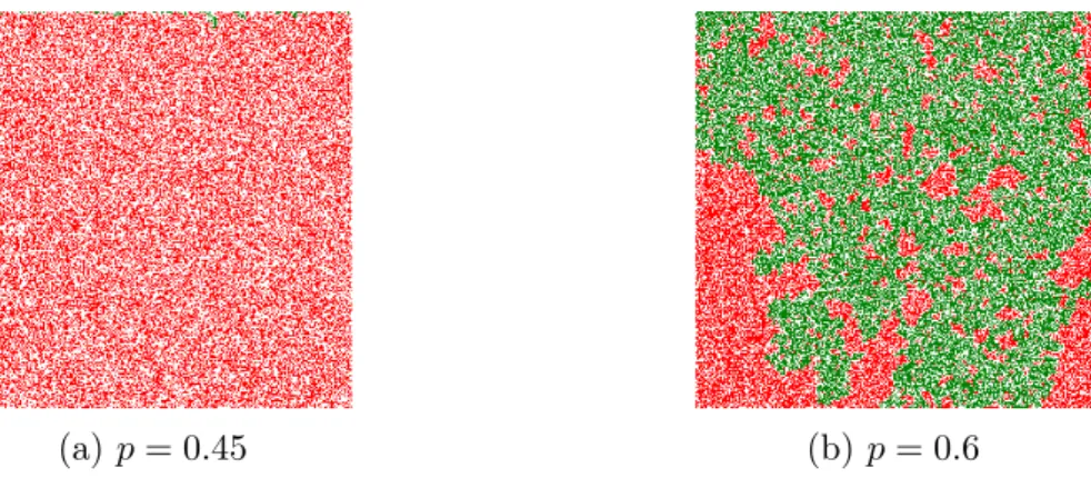
The percolation model, is a model meant to study the spread of fluid through a random medium. More precisely, assume that the medium of interest has different channels with different wideness. The fluid will only spread through channels that are wide enough. A question of interest here is whether the fluid can reach the origin starting from outside a large region.
The first mathematical model of percolation was introduced in Broadbent and Ham-mersley (1957). More precisely, the channels are the edges or bonds between adjacent
sites on the integer lattice in the plane Z2. Each bond is passable with probability p
(and hence blocked with probability q = 1 p), and all the bonds are independent of
each other. The fundamental question of percolation theory is for which p is there an infinite open cluster?
(a) p = 0.45 (b) p = 0.6
Figure 1.1: Illustration of percolation on a square lattice of size 500 ⇥ 500. Bonds are red if open, white if blocked and percolation paths are in green.
If we set E1 to be the event that there is an infinite open cluster, then it is trivial
P(E1) is 0 or 1 for any p. Hence, it is natural to expect the existence of a phase
transition around some critical threshold pc.
Inspired by a line of works, to name Harris (1960), Kesten (1980) proved the long conjectured result that the critical probability is exactly 1/2. In other words, the ob-served phase transition on the square lattice is the following:
• For p > 1/2, there is with probability one a unique infinite open cluster. • For p < 1/2, just the opposite occurs, and percolation is impossible. Connectivity in the Erdős-Rényi Model
In their seminal paper, Erdős and Rényi (1960) introduced and studied several properties of what we call today the Erdős-Rényi (ER) Model as one of the most popular models in graph theory.
In the ER model G(n, p), n nodes are constructed randomly, then each edge is included in the graph with probability p independent from every other edge. This provides us with a model described by a single parameter. This model has been (and still is) a source of intense research activity, in particular due to its phase transition phenomenon. A very interesting question is related to connectivity of this graph.
Obviously, as p grows the graph is most likely to be connected. One may wonder what is the probability above which the graph is connected almost surely. Erdős and Rényi (1960) show the existence of a sharp phase transition for the described phenomenon as
n tends to infinity. For any ✏ 2 (0, 1), they prove the following
• For p < (1 ✏)log n
n , then a graph in G(n, p) almost surely contains isolated vertices,
and thus is disconnected.
• For p > (1 + ✏)log n
n , then a graph in G(n, p) is almost surely connected.
Thus log n
n is a sharp threshold for the connectivity of G(n, p).
There is some similarity between percolation and connectivity in the ER Model. Indeed, we may see the latter problem as a percolation problem on the complete graph instead of the lattice. One may also notice that the critical probability in the ER Model is smaller than the one in percolation and the difference is mainly due to their different geometric structures - more degrees of freedom are allowed in the ER Model. The precise link between the two problems is beyond the scope of this introduction.
Spiked Wigner Model
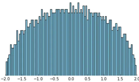
Random matrices are in the heart of many problems in multivariate statistics such as estimation of covariance matrices and low rank matrix estimation, to name a few. We present here a phase transition phenomenon in the Wigner Model.
Wigner was the first to observe a very interesting property of the spectrum of ran-dom matrices. Suppose that W is drawn from the n ⇥ n GOE (Gaussian Orthogonal
Ensemble), i.e. W is a random symmetric matrix with off-diagonal entries N (0,1
n),
diagonal entries N (0, 2
n), and all entries independent (except for symmetry Wij = Wji).
Set µn to be the empirical spectral measure of W such that
µn(A) =
1
1.2. INTERACTION WITH OTHER DISCIPLINES 9
Figure 1.2: The empirical spectral distribution of a matrix drawn from the 1500 ⇥ 1500 GOE.
The limit of the empirical spectral measure for Wigner matrices, as n tends to infinity, is the Wigner semicircle distribution, as described by Wigner (1958). The semicircle distribution is supported on [ 2, 2] and is given by the density
µ(x) = 1
2⇡ p
4 x2, 8x 2 [ 2, 2].
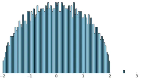
This phenomenon is more general and universal in the sense that it holds not neces-sarily for matrices with Gaussian entries. From a physical point of view, we may view the eigenvalues of W as an interacting system where it is possible to characterize these interactions precisely. The previous result, in particular, states that the eigenvalues are confined in the compact set [ 2, 2] with high probability (this holds even almost surely). A very interesting question is about the behaviour of the spectrum of W under an external action. More precisely, for > 0, and a spike vector x such that kxk = 1 , we define the spiked Wigner model as follows:
Y = xx>+ W.
As above, it is not difficult to observe that the top eigenvalue of Y is 2 if = 0 and
that it tends to infinity as goes to infinity. Hence, we may wonder at which power of the spike the spectrum gets affected. This question was solved by Féral and Péché (2007) where a new phase transition phenomenon arises as n tends to infinity.
• For 1, the top eigenvalue of Y converges almost surely to 2. • For > 1, the top eigenvalue converges almost surely to + 1/ > 2.
It was further shown in Benaych-Georges and Nadakuditi (2011) that the top (unit-norm) eigenvector ˆx of Y has non-trivial correlation with the spike vector almost surely,
if and only if > 1. This phase transition is probably at the heart of a better
Figure 1.3: The empirical spectral distribution of a spiked Wigner matrix with n = 1500 and = 2.
distinguish the presence of a spike from its absence. In Perry et al. (2018), this question is studied in detail and it turns out that, under the Gaussian random spike, the spectral test based on the top eigenvalue of Y is, in a certain sense, the best test that one should use in order to test the presence of a spike.
This result is exciting but also alarming. Indeed, the spiked model is a simple model to study the performance of Principal Component Analysis (PCA). Basically, we assume the presence of a low rank signal corrupted by some noise, and want to recover the underlying signal. The previous results show that, in the regime where < 1, there is no hope to capture non-trivial correlation with the signal and hence the resulting PCA is meaningless. Such facts are not always known to practitioners and we believe that a good use and interpretation of PCA should always start with a safety test asserting whether PCA is meaningful or not.
Interaction with optimization
Statistics and Learning Theory are intimately linked with optimization when it comes to algorithms. Indeed, in Learning Theory, a classical problem is to minimize some empirical risk. In order to evaluate the performance of a predictor or a classifier we rely on a specific choice of some loss function and evaluate the performance with respect to it. In that sense the notion of goodness of training is relative to the choice of loss. As long as we can optimize the objective loss function, we may be able to derive a good predictor that is usually optimal in some sense.
For statisticians, the main interest is statistical accuracy. It is still important to wonder whether we can in practice find an optimizer. For this purpose, we rely on the wealth of results developed by the optimization community that is mostly designed for convex objective functions (where we have existence of global minima) defined on convex sets. Hence, as long as the goal is to minimize some convex function on a convex set, we may assume given the corresponding minimizer.
Unfortunately, in many important problems convexity is not granted. A popular approach is to convexify the objective function and to optimize its convex counterpart. This is one important example of the influence of optimization on statistics. By doing
1.2. INTERACTION WITH OTHER DISCIPLINES 11 so, one still has to prove that a good solution of the convex problem leads to a good predictor for the original problem. In classification, SVM and boosting are examples supporting that the convexification trick can be optimal. The previous remark does not hold in general. As an example, Sparse PCA is a non-convex problem where its SDP relaxation (cf. d’Aspremont et al. (2005)) leads to a strict deterioration of the rate of estimation compared to a solution of the original problem. In simple words, convexification is not always optimal.
Most interestingly, the interplay between statistics and optimization becomes more beneficial when combining both realms. A popular approach handling non-convex prob-lems is given by variants of greedy descents over the objective function. This is usually how iterative algorithms are designed. Some popular examples are Lloyds for K-means clustering (Lloyd (1982)) and Iterative Hard Thresholding for sparse linear regression (Shen and Li (2017); Foucart and Lecué (2017); Liu and Barber (2018)).
These algorithms are non-convex counterparts of gradient descent methods. One may argue that studying the statistical performance of iterative algorithms can be richer than analyzing minimizers of objective functions. We discuss below this fact.
• Advantages of iterative algorithms:
It is common in the statistical community to evaluate the performance of esti-mators given as solutions of optimization problems. In practice, we do not have access to one of the optimizers but only to an approximation. The corresponding approximation error is missing in the statistical analysis and is referred to as the optimization error. By studying iterative algorithms, we get a precise control of both errors after a certain number of steps.
The optimization error can be made as small as possible by running a large number of iterations. Usually the number of iterations is set at some precision level. While the optimization error is vanishing and depends on the speed of the algorithm, the statistical error is intrinsic. Hence, the latter is in all cases a lower bound of the global error. That being said, there is no need to run an infinite number of iterations and we can always stop the algorithm once the statistical accuracy is reached. Combining statistics and optimization, we may consider early stopping rules saving time and efforts from the optimization side.
Following the previous fact, there is no need of global convergence of the algorithm. Existence of global minima is not even required. Indeed, as long as local minima of the objective function are below the optimal statistical error, then the algorithm succeeds.
To sum up, on one hand, iterative algorithms may tolerate non-convexity for some statistical problems, while on the other hand statistical limits and assumptions allow for more flexibility and improvements of the algorithms.
• Defects of iterative algorithms:
Although the benefits of combining optimization and statistics are numerous, there are still some drawbacks in using iterative algorithms. The first one is probably related to ignoring which deterministic descent algorithm to mimic in order to con-struct an iterative procedure. Objective function minimization is a good guideline for that purpose, as long as we only care about the statistical performance. To
the best of our knowledge, the choice of iterative methods is empirical and there is no general rule to master it.
Another drawback and probably the most limiting part in the analysis of iterative algorithms is the dependence between the steps. Indeed, while the noise is usually assumed to have independent entries, after one iteration the estimator usually starts depending on the noise in a complex way. It is not always trivial to handle these dependencies but in some important examples we can use the contraction of the objective function in order to get around it, cf. for example, Lu and Zhou (2016).
We conclude this section by mentioning a potential direction to explore as a consequence of the interplay between the fields of Optimization and Statistics. It is well known that in both fields, the notion of adaptivity is of high importance. An adaptive algorithm solving an optimization problem is probably not adaptive from a statistical perspective and vice versa. Simultaneous analysis, through iterative algorithms for instance, may lead to a more accurate notion of adaptivity.
1.3 Variable Selection and Clustering
Variable selection is an important task in Statistics that has many applications. Consider the linear regression model in high dimensions, and assume that the underlying vector
✓ is sparse. There are three questions of interest that could be treated independently.
• Detection: Test the presence of a sparse signal against the hypothesis that the observation is pure noise.
• Estimation: Estimate the sparse signal vector.
• Support recovery: Recover the set of non-zero variables (support of the true sparse signal).
In what follows, the question of variable selection is equivalent to support recovery. While detection and support recovery require additional separation conditions, in order to get meaningful results, it is not the case for estimation. The three problems cannot always be compared in terms of hardness. It is obvious that detection is easier than support recovery in the sense that it requires weaker separation conditions, but there are no general rules to compare these tasks.
At this stage, we want to emphasize that these three tasks may be combined for a specific purpose but they can also be used independently following the statistical ap-plication. Let us consider an illustrative example of these tasks. An internet service provider routinely collects statistics of server to determine if there are abnormal black-outs. While this monitoring is performed on a large number of servers, only very few servers are believed to be experiencing problems if there are any. This represents the sparsity assumption. The detection problem is then equivalent to determining if there are any anomalies among all servers; the estimation problem is equivalent to associating weights (probability of failure) to every server, while support recovery is equivalent to identifying the servers with anomalies.
1.3. VARIABLE SELECTION AND CLUSTERING 13 Probably one of the most exciting applications of high-dimensional variable selection is in genetic epidemiology. Typically, the number of subjects n, is in thousands, while
p ranges from tens of thousands to hundreds of thousands of genetic features. The
number of genes exhibiting a detectable association with a trait is extremely small in practice. For example, in disease classification, it is commonly believed that only tens of genes are responsible for a disease. Selecting tens of genes helps not only statisticians in constructing a more reliable classification rule, but also biologists to understand molecular mechanisms.
Apart from its own interest, variable selection can be used in estimation procedures. For instance it can be used as a first step in sparse estimation reducing the dimension of the problem. The simple fact that estimating a vector on its true support has a significantly smaller error than on the complete vector, has encouraged practitioners to proceed to variable selection as a first step. Wasserman and Roeder (2009) is an example of works studying the theoretical aspects of methods in the same spirit. Long story short, the main idea of this approach is to first find a good sparse estimator and then keep its support. This step is also known as model selection. Once the support is estimated, the dimension of the problem is much smaller than the initial dimension p. The second step is then to estimate the signal solving a simple least-square problem on the estimated support.
Examples of Variable Selection methods
The issues of variable selection for high-dimensional statistical modeling has been widely studied in last decades. We give here a brief summary of some well-known procedures. All these procedures are thresholding methods. Logically, selecting a variable is only possible if we can distinguish it from noise. As long as we can estimate the noise level, the variables that are above this level are more likely to be relevant. This also explains why the threshold usually depends on the noise and not necessarily on the significant variables.
In order to present some of these thresholding methods, assume that we observe
x2 Rp, such that
x = ✓ + ⇠,
where ✓ is a sparse vector, and ⇠ is a vector of identically distributed noise variables, not necessarily independent. A thresholding procedure typically returns an estimated
set ˆS of the form
ˆ
S = {j : |xj| > t(x)},
where xj is the j-th component of x. Note that the threshold t(.) may depend on
the vector x. Here are examples of thresholding procedures, where the two first are deterministic while the others are data-dependent.
• Bonferroni’s procedure: Bonferroni’s procedure with family-wise error rate (FWER) at most ↵ 2 (0, 1) is the thresholding procedure that uses the threshold
t(x) = F 1(1 ↵/2p).
We use the abusive notation F 1 to denote the generalized inverse of the c.d.f of
• Sidák’s procedure (Šidák (1967)): This procedure is more aggressive (i.e. gives higher threshold) than Bonferroni’s procedure. It uses the threshold
t(x) = F 1((1 ↵/2)1/p).
Consider the non-increasing arrangement of coordinates of x in absolute value such that
|x|(1) · · · |x|(p). The next procedures are data-dependent and are shown to be
strictly more powerful than Bonferroni’s procedure.
• Holm’s procedure (Holm (1979)): Let k be the largest index such that
|x|(i) F 1(1 ↵/2(p i + 1)), 8i k.
Holm’s procedure with FWER controlled at ↵ is the thresholding procedure that uses
t(x) = |x|(k). (1.1)
• Hochberg’s procedure (Hochberg (1988)): More aggressive than Holm’s, the cor-responding threshold is given by (1.1) where k is the largest index i such that
|x|(i) F 1(1 ↵/2(p i + 1)).
Theoretical properties of these methods, in a more general setting, are analyzed in the recent work of Gao and Stoev (2018).
Community Detection
Learning community structures is a central problem in machine learning and computer science. The simplest clustering setting is the one where we observe n agents (or nodes) that are partitioned into two classes. Depending on available data, we may proceed differently. When observed data is interactions among agents (e.g., social, biological, computer or image networks), then clustering is node-based. While, when observed data is spacial position of agents, then clustering is vector-based. In both cases, the goal is to infer, from the provided observations, communities that are alike or complementary. A very popular model for the first case is the Stochastic Block Model (Holland et al. (1983)), while the two component Gaussian mixture model is the equivalent for the second case. The problem of community recovery can be reformulated as recovering the set of labels belonging to the same class and hence can be seen as a variable selection problem.
As the study of community detection grows at the intersections of various fields, the notions of clusters and the models vary significantly. As a result, the comparison and validation of clustering algorithms remains a major challenge.
Stochastic Block Model (SBM)
The SBM has been at the center of attention in a large body of literature. It can be seen as an extension of the ER model, described previously. Recall that in the ER model, edges are placed independently with probability p, providing a model described by a single parameter. It is however well known to be too simplistic to model real networks,
1.3. VARIABLE SELECTION AND CLUSTERING 15 in particular due to its strong homogeneity and absence of community structure. The SBM is based on the assumption that agents in a network connect not independently but based on their profiles, or equivalently, on their community assignment. Of particular interest is the SBM with two communities and symmetric parameters, also known as the planted bisection model, denoted here by G(n, p, q), with an integer n denoting the number of vertices.
More precisely, each node v in the graph is assigned a label v 2 { 1, 1}, and each
pair of nodes (u, v) is connected with probability p within the clusters of labels and q across the clusters. Upon observing the graph (without labels), the goal of community detection is to reconstruct the label assignments. Of course, one can only hope to recover the communities up to a global flip of labels. When p = q, it is clearly impossible to recover the communities, whereas for p > q or p < q, one may hope to succeed in certain regimes. While this is a toy model, it captures some of the central challenges for community detection. In particular, it represents a phase transition similar to the ER model. In the independent works of Abbe et al. (2014) and Mossel et al. (2015), the phase transition of exact recovery is characterized precisely. For any ✏ > 0, we observe the following as n tends to infinity,
• For pp pq < (1 ✏)q2 log n
n , then exact recovery of labels in G(n, p, q) is
impos-sible.
• For pp pq > (1+✏)q2 log n
n , then exact recovery of labels in G(n, p, q) is possible
and is achieved through a polynomial time method.
One method achieving the sharp phase transition is based on a spectral method followed by a rounding procedure. In order to get more intuition on the construction of such a method, let us observe that the graph adjacency matrix A can be decomposed as follows
A = p + q
2 11
>+ p q
2 ⌘⌘
>+ W,
where 1 is the vector of ones in Rn, ⌘ 2 { 1, 1}n is the vector of labels up to a sign
change and W is a centered sub-Gaussian random matrix with independent entries. The first term, also known as the mean component can be removed if p + q is known or simply by projecting the adjacency matrix on the orthogonal of 1. As a consequence, the observation A has a similar behaviour as the Spiked Wigner model. It can be shown that spectral methods are efficient to detect the presence of the planted bisection structure and also to get non-trivial correlation with the vector of labels. The rounding step can be seen as a cleaning step that helps finding the exact labels once a non-trivial correlation is captured.
Gaussian Mixture Model (GMM)
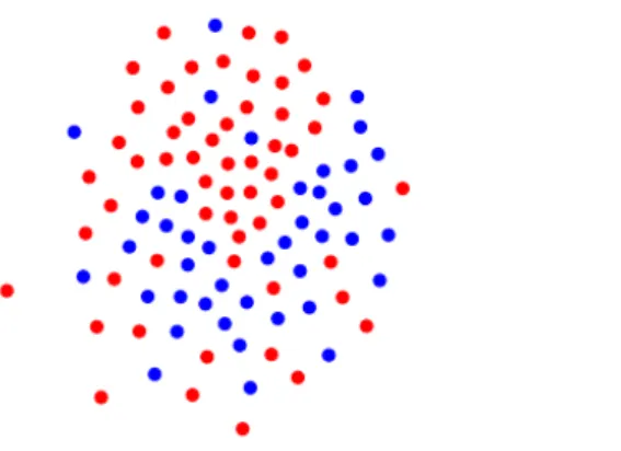
The Gaussian Mixture Model is one of the most popular statistical models. Of particular interest is the two component Gaussian Mixture Model with two balanced communities.
Similary to SBM, assume that ⌘ 2 { 1, 1}n is a vector of labels. In a GMM with
labels ⌘, the random vectors Yi are assumed to be independent and to follow a Gaussian
distribution with variance 1 centered at ✓1 if ⌘i = 1 or centered at ✓2 if ⌘i = 1,
to the same group are close to each other and we may rely on distances between the observations to cluster them.
Figure 1.4: A two-dimensional projection of a two component Gaussian mixture with
n = 100 and p = 1000.
As for SBM, spectral methods used for GMM are inspired by the following fact.
Notice that the observation matrix Y 2 Rp⇥n can be decomposed as follows
Y = ✓1+ ✓2
2 1
>+✓1 ✓2
2 ⌘
>+ W,
where W is a centered Gaussian random matrix with independent columns. The mean
component ✓1+✓2
2 1> can be handled in the same way as for SBM. As a consequence,
clustering is possible when k✓1 ✓2k is large enough. The observation Y can be viewed
as an asymmetric equivalent of the Spiked Wigner Model. We refer the reader to the recent work of Banks et al. (2018) for phase transitions in this model.
Apart from community detection, the problem of center estimation in GMM is of high interest as well. Although many iterative procedures, in the same spirit as K-means, operate a center estimation step, it is not always true that the center estimation is necessary to achieve exact recovery. As we will argue in Chapter 6 the two problems may be considered independently.
Chapter 2
Overview of the Results
This thesis deals with the following statistical problems: Variable selection in high-Dimensional Linear Regression, Clustering in the Gaussian Mixture Model, Some effects of adaptivity under sparsity and Simulation of Gaussian processes. The goal of this chapter is to provide a motivation for these statistical problems, to explain how these areas are connected and to give an overview of the results derived in the next chapters. Each chapter can be read independently of the others.
2.1 Variable Selection in High-Dimensional Linear
Regression
In recent years, the problem of variable selection in high-dimensional regression models has been extensively studied from the theoretical and computational viewpoints. In making effective high-dimensional inference, sparsity plays a key role. With regard to variable selection in sparse high-dimensional linear regression, the Lasso, Dantzig selector, other penalized techniques as well as marginal regression were analyzed in detail. In some cases, practitioners are more interested in the pattern or support of the signal rather than its estimation. It turns out, that the problem of variable selection or support recovery are highly dependent on the separation between entries of the signal on its support and zero. One may define optimality in a minimax sense for this problem. In particular, the study of phase transitions in support recovery with respect to the separation parameter is of high interest. The model of interest is the one of high-dimensional linear regression
Y = X✓ + ⇠.
When X is an orthogonal matrix the model corresponds to the sparse vector model, while when X is random it corresponds to noisy Compressed Sensing. Some papers on this topic include Meinshausen and Bühlmann (2006); Candes and Tao (2007); Wainwright (2009b); Zhao and Yu (2006); Zou (2006); Fan and Lv (2008); Gao and Stoev (2018).
Chapter 3 is devoted to derive non-asymptotic bounds for the minimax risk of
sup-port recovery under expected Hamming loss in the Gaussian mean model in Rd for
classes of s-sparse vectors separated from 0 by a constant a > 0. Namely, we study the problem of variable selection in the following model:
Yj = ✓j+ ⇠j, j = 1, . . . , d,
where ⇠1, . . . , ⇠d are i.i.d. standard Gaussian random variables, > 0 is the noise
level, and ✓ = (✓1, . . . , ✓d) is an unknown vector of parameters to be estimated. For
s 2 {1, . . . , d} and a > 0, we assume that ✓ is (s, a)-sparse, which is understood in the
sense that ✓ belongs to the following set:
⇥d(s, a) = ✓2 Rd : there exists a set S ✓ {1, . . . , d} with at most s elements
such that |✓j| a for all j 2 S, and ✓j = 0 for all j /2 S .
We study the problem of selecting the relevant components of ✓, that is, of estimating the vector
⌘ = ⌘(✓) = I(✓j 6= 0) j=1,...,d,
where I(·) is the indicator function. As estimators of ⌘, we consider any measurable
functions ˆ⌘ = ˆ⌘(Y1, . . . , Yd)of (Y1, . . . , Yd)taking values in {0, 1}d. Such estimators will
be called selectors. We characterize the loss of a selector ˆ⌘ as an estimator of ⌘ by the Hamming distance between ˆ⌘ and ⌘, that is, by the number of positions at which ˆ⌘ and
⌘ differ: |ˆ⌘ ⌘| , d X j=1 |ˆ⌘j ⌘j| = d X j=1 I(ˆ⌘j 6= ⌘j).
Here, ˆ⌘j and ⌘j = ⌘j(✓) are the jth components of ˆ⌘ and ⌘ = ⌘(✓), respectively. The
expected Hamming loss of a selector ˆ⌘ is defined as E✓|ˆ⌘ ⌘|, where E✓ denotes the
expectation with respect to the distribution P✓ of (Y1, . . . , Yd). We are interested in the
minimax risk
inf
˜
⌘ ✓2⇥supd(s,a)E✓|˜⌘ ⌘|.
In some cases, we get exact expressions for the non-asymptotic minimax risk as a function of d, s, a and find explicitly the corresponding minimax selectors. These results are extended to dependent or non-Gaussian observations and to the problem of crowdsourcing. Analogous conclusions are obtained for the probability of wrong recovery of the sparsity pattern. As corollaries, we characterize precisely an asymptotic sharp phase transition for both almost full and exact recovery. We say that almost full recovery is possible if there exists a selector ˆ⌘ such that
lim
d!1✓2⇥supd(s,a)
1
sE✓|˜⌘ ⌘| = 0.
Moreover, we say that exact recovery is possible if there exists a selector ˆ⌘ such that lim
d!1✓2⇥supd(s,a)
E✓|˜⌘ ⌘| = 0.
Among other results, we prove that necessary and sufficient conditions for almost full and exact recovery are respectively
a > p2 log(d/s 1)
and
2.1. VARIABLE SELECTION IN HIGH-DIMENSIONAL LINEAR REGRESSION19 Moreover, we propose data-driven selectors that provide almost full and exact recovery adaptively to the parameters of the classes.
As a generalization to high-dimensional linear regression, we study in Chapter 4 the problem of exact support recovery in noisy Compressed Sensing. Assume that we have
the vector of measurements Y 2 Rn satisfying
Y = X✓ + ⇠
where X 2 Rn⇥p is a given design or sensing matrix, ✓ 2 Rp is the unknown signal, and
> 0. Similarily to the Gaussian sequence model case, we assume that ✓ belongs to
⇥p(s, a).We are interested in the Hamming minimax risk, and therefore in sufficient and
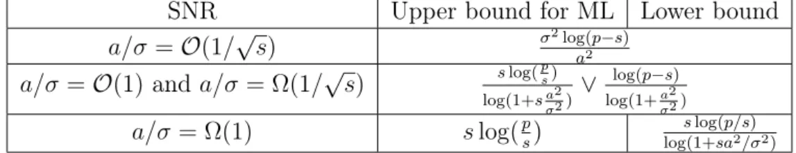
necessary conditions for exact recovery in Compressed Sensing. Table 2.1 summarizes
SNR Upper bound for ML Lower bound
a/ =O(1/ps) 2log(p s)a2
a/ =O(1) and a/ = ⌦(1/ps) s log(ps)
log(1+sa22) _
log(p s) log(1+a22)
a/ = ⌦(1) s log(ps) log(1+sas log(p/s)2/ 2)
Table 2.1: Phase transitions in Gaussian setting.
known sufficient and necessary conditions for exact recovery in the setting where both
X and ⇠ are Gaussian.
We propose an algorithm for exact support recovery in the setting of noisy com-pressed sensing where all entries of the design matrix are i.i.d standard Gaussian. This algorithm is the first polynomial time procedure to achieve the same conditions of exact recovery as the exhaustive search (maximal likelihood) decoder that was studied in Rad (2011), Wainwright (2009a). In particular, we prove that, in the zone a/ = O(1), our sufficient condition for exact recovery has the form
n = ⌦ ✓ s log⇣p s ⌘ _ 2log(p s) a2 ◆ ,
where we write xn = ⌦(yn) if there exists an absolute constant C > 0 such that xn
Cyn. Our procedure has an advantage over the exhaustive search of being adaptive
to all parameters of the problem and computable in polynomial time. The core of our analysis consists in the study of the non-asymptotic minimax Hamming risk of variable selection. This allows us to derive a procedure, which is nearly optimal in a non-asymptotic minimax sense. We develop its adaptive version, and propose a robust variant of our method to handle datasets with outliers and heavy-tailed distributions of observations. The resulting polynomial time procedure is near optimal, adaptive to all parameters of the problem and also robust.
Another topic of interest is the interplay between estimation and support recovery. As described previously, and depending on applications, practitioners may be interested either in accurate estimation of the signal or recovering its support. It is not clear how the two problems are connected. When the support of the signal is known, one
may achieve better rates of estimation but it is not clear whether the knowledge of the support is necessary for that.
A fairly neglected problem by practitioners is the bias in high-dimensional estimation.
Despite their popularity, the l1-regularization methods suffer from some drawbacks. For
instance, it is well known that penalized estimators suffer from an unavoidable bias as pointed out in Zhang and Huang (2008), Bellec (2018). A sub-optimal remedy is to threshold the resulting coefficients as suggested in Zhang (2009). However, this approach requires additional tuning parameters, making the resulting procedures more complex and less robust. It turns out that under some separation of the components this bias can be removed. Zhang (2010) propose a concave penalty based estimator in order to deal with the bias term. A variant of this method that is adaptive to sparsity is given in Feng and Zhang (2017).
Alternatively, other techniques were introduced through greedy algorithms such as Orthogonal Matching Pursuit: Cai and Wang (2011); Joseph (2013); Tropp and Gilbert (2007); Zhang (2011b). For Forward greedy algorithm, also referred to as matching pur-suit in the signal processing community, it was shown that the irrepresentable condition
of Zhao and Yu (2006) for l1-regularization is necessary to effectively select features.
For Backward greedy algorithm, although widely used by practitioners, not much was known concerning its theoretical analysis in the literature before Zhang (2011a). A combination of these two algorithms is presented in Zhang (2011a) and turns out to be successful removing the bias when it is possible. Again, we emphasize that a pre-cise characterization of necessary and sufficient conditions for the bias to be removed is missing and will certainly complement the state of the art results.
Chapter 5 is devoted to the interplay between estimation and support recovery. We introduce a new notion of scaled minimaxity for sparse estimation in high-dimensional linear regression model. The scaled minimax risk is given by
inf ˆ ✓ sup ✓2⇥d(s,a) E✓ ⇣ kˆ✓ ✓k2⌘,
where the infimum is taken over all possible estimators ˆ✓ and k.k is the `2-norm,. We
present more optimistic lower bounds than the one given by the classical minimax theory and hence improve on existing results. We recover the sharp result of Donoho et al. (1992) for the global minimaxity in the Gaussian sequence model as a consequence of our study, namely
inf ˆ ✓ sup |✓|0s E✓ ⇣ kˆ✓ ✓k2⌘= 2 2s log(d/s)(1 + o(1)) as s d ! 0. (2.2)
Here |.|0 is the number of non-zero components and E✓ denotes the expectation with
respect to the distribution of Y in the Gaussian sequence model. Fixing the scale of the signal-to-noise ratio, we prove that estimation error can be much smaller than the global minimax error. We also study sufficient and necessary conditions for an estimator ˆ
✓ to achieve exact estimation that corresponds in the Gaussian sequence model to the
following property: lim s/d!0 sup ✓2⇥d(s,a) E✓ ⇣ kˆ✓ ✓k2⌘ 2s = 1.
2.2. CLUSTERING IN GAUSSIAN MIXTURE MODEL 21 The notion of exact estimation is closely related to the bias of estimation, since achieving exact estimation is only possible if the bias is avoidable. Finally, we construct a new optimal estimator for the scaled minimax sparse estimation and derive its adaptive variant.
Among other findings, we show that exact support recovery is not necessary to achieve the scaled minimax error. Indeed, in Chapter 5, we obtain a new phase transition related to sparsity. Recall that we show in Chapter 3 that the necessary and sufficient condition to achieve exact recovery is given by
a > p2 log(d s) + p2 log(s),
cf. (2.1). To achieve exact estimation, we prove that a necessary condition is given by
a > p2 log(d/s 1) + 2 log log(d/s 1) + p2 log log(d/s 1).
Hence exact recovery is not necessary for exact estimation. In fact, when s log(d)
then exact estimation is easier and when s ⌧ log(d) exact recovery becomes easier. This shows that there is no direct implication of exact recovery on exact estimation, and the latter task should be considered as a separate problem.
2.2 Clustering in Gaussian Mixture Model
Gaussian Mixture Model (GMM) is one of the most popular vector clustering models. The simple case of two components mixture is modeled as follows:
Yi = ⌘i✓ + ⇠i, 8i = 1, . . . , n, (2.3)
where ✓ 2 Rp is the center vector, ⌘ = (⌘
1, . . . , ⌘n) 2 { 1, 1}n is the labels vector
and (⇠i)1in is a sequence of standard independent random Gaussian vectors. Two
im-portant questions arising in this model are related to center estimation and community detection. Performance guarantees for several algorithmic alternatives have emerged, in-cluding expectation maximization (Dasgupta and Schulman (2007)), spectral methods (Vempala and Wang (2004); Kumar and Kannan (2010); Awasthi and Sheffet (2012)), projections (random and deterministic in Moitra and Valiant (2010); Sanjeev and Kan-nan (2001)) and the method of moments (Moitra and Valiant (2010)).
While Moitra and Valiant (2010) and Mixon et al. (2016) are interested in center estimation, Vempala and Wang (2004); Kumar and Kannan (2010); Awasthi and Sheffet (2012) are interested in recovering correctly the clusters. We only focus on the latter question in this manuscript.
The paper of Lu and Zhou (2016) is one of the first works that study theoretical guarantees of Lloyd’s algorithm in order to recover communities in the sub-Gaussian Mixture Model. It, particularly, succeeds to handle the dependence between different steps of the latter algorithm. Recently, Fei and Chen (2018) and Giraud and Verzelen (2018) have investigated the clustering performance of SDP relaxed K-means in the setting of sub-Gaussian Mixture Model. After identifying the appropriate signal-to-noise ratio (SNR), that is different from the one given by Lu and Zhou (2016) when p > n, Giraud and Verzelen (2018) prove that the misclassification error decays exponentially
fast with respect to this SNR. These recovery bounds for SDP relaxed K-means improve upon the results previously known in the GMM setting.
In high dimensional regime, the exact recovery phase transition is not known. Also, in the same regime, there is a strict performance gap between known results for fast iterative algorithms and SDP relaxation methods. It is of interest to know whether this gap is crucial or not. Eventual positive answers will complement the state of the art results.
In Chapter 6, we consider the problem of exact recovery of clusters in the two
components Gaussian Mixture Model (2.3). We denote by P(✓,⌘) the distribution of Y
and by E(✓,⌘) the corresponding expectation. We assume that (✓, ⌘) belongs to the set
⌦ ={✓ 2 Rp :k✓k } ⇥ { 1, 1}n,
where > 0 is a given constant. We consider the following Hamming loss of selector ˆ⌘:
r(ˆ⌘, ⌘) := min
⌫2{ 1,1}|ˆ⌘ ⌫⌘|,
and its expected loss defined as E(✓,⌘)r(ˆ⌘, ⌘). We are interested in the following minimax
risk: := inf ˜ ⌘ (✓,⌘)2⌦sup 1 nE(✓,⌘)r(˜⌘, ⌘), where inf ˜
⌘ denotes the infimum over all estimators ˜⌘ with values in { 1, 1}
n. After
identifying the appropriate signal-to-noise ratio (SNR) rn of the problem:
rn=
2/ 2
p 2
/ 2+ p/n,
our main contribution is to prove that
⇣ e r2
n(1/2+o(1)),
where o(1) denotes a bounded sequence that vanishes as n goes to infinity. As a conse-quence we recover the sharp phase transition for exact recovery in the Gaussian mixture
model. Namely, we show that the phase transition occurs around the threshold = ¯n
such that ¯2 n= 2 ✓ 1 + r 1 + 2p n log n ◆ log n. (2.4)
Moreover, we propose a procedure achieving this threshold. It is a variant of Lloyd’s iterations initialized by a spectral method. This procedure is a fully adaptive, rate opti-mal and computationally simple. The main difference in the proposed method compared to the classical EM style algorithms is the following. Most of these algorithms are based on estimating the center at each step, and this is exactly where they loose optimality. In the high SNR regime, there is no hope to achieve even a non-trivial correlation with the true center vector, but exact recovery of labels is still possible. This means that in high dimension, any algorithm relying on estimation of the center must be suboptimal. To the best of our knowledge, the suggested procedure is the first fast method to achieve optimal exact recovery. In addition, it achieves sharp optimality since we derive the threshold of (2.4) with precise constant. Moreover, this procedure is as fast as any spectral method in terms of complexity. In other words, the proposed procedure takes the best both of the realm of SDP and of the spectral methods.
2.3. ADAPTIVE ROBUST ESTIMATION IN SPARSE VECTOR MODEL 23
2.3 Adaptive robust estimation in sparse vector model
For the sparse vector model
Y = ✓ + ⇠,
estimation of the target vector ✓ and of its `2-norm are classical problems that are of
interest to the statistical community. In the case where ⇠ is Gaussian and is known,
these questions are well understood. A crucial issue arises when the noise level and/or the noise distribution are unknown. Then, one is also interested in the problem of estimation of .
The classical Gaussian sequence model corresponds to the case where the noise ⇠ is standard Gaussian, and the noise level is known. Then, the optimal rate of estimation of ✓ under the quadratic loss in a minimax sense on the class of s-sparse vectors is given in (2.2) and it is attained by thresholding estimators, cf. Donoho et al. (1992). Also, for the Gaussian sequence model with known , minimax optimal estimator of the norm k✓k as well as the corresponding minimax rate are available from Collier et al. (2017). It remains to characterize the effects of ignoring some of these parameters on different minimax estimation rates.
We emphasize here, that the parameter ✓ can play two roles. Either it is the param-eter of interest to estimate or a nuisance paramparam-eter if we are interested in estimation
of 2. Chen et al. (2018) explore the problem of robust estimation of variance and of
covariance matrix under Huber’s contamination model. This problem has similarities with estimation of noise level in our setting. Another aspect of robust estimation of scale is analyzed by Wei and Minsker (2017) who consider classes of heavy tailed dis-tributions, rather than the contamination model. The main aim in Wei and Minsker (2017) is to construct estimators having sub-Gaussian deviations under weak moment assumptions. In the sparse linear model, estimation of variance is discussed in Sun and Zhang (2012) where some upper bounds for the rates are given, while estimation of the
`2-norm is discussed in Carpentier et al. (2018). We also mention the recent papers of
Collier et al. (2018); Carpentier and Verzelen (2019) that discuss estimation of other
functionals than the `2-norm in the sparse vector model when the noise is Gaussian with
unknown variance.
In Chapter 7, we consider separately the setting of Gaussian noise, or when the
distribution of ⇠i and the noise level are both unknown. For the unknown
distribu-tion of ⇠1, we denote by P⇠ the unknown distribution of ⇠1 and consider two types of
assumptions. Either P⇠ belongs to a class Ga,⌧, i.e. for some a, ⌧ > 0,
P⇠2 Ga,⌧ iff E(⇠1) = 0, E(⇠12) = 1 and 8t 2, P |⇠1| > t 2e (t/⌧ )
a
, which includes for example sub-Gaussian distributions (a = 2), or to a class of
distribu-tions with polynomially decaying tails Pa,⌧, i.e. for some ⌧ > 0 and a 2,
P⇠2 Pa,⌧ iff E(⇠1) = 0, E(⇠12) = 1 and 8t 2, P |⇠1| > t)
⇣⌧ t
⌘a
.
We are interested in the following maximal risk functions over classes of s-sparse vectors: sup |✓|0s v u u tE✓,P⇠, kˆ✓ ✓k!2 , (2.5)