1
Comparing transient and steady-state methods for the thermal
1conductivity characterization of a borehole heat exchanger field in
2Bergen, Norway
34
Nicolò Giordano 1,2, Jessica Chicco 2, Giuseppe Mandrone 2, Massimo Verdoya 3, Walter H. Wheeler 4 5
1 Institut national de la recherche scientifique – Centre Eau Terre Environnement, 490 Rue de la Couronne, G1K 9A9,
6
Québec (QC), Canada
7
2 Dipartimento di Scienze della Terra, Università di Torino, Via Valperga Caluso, 35 10125 Torino, Italy
8
3 Dipartimento di Scienze della Terra, dell’Ambiente e della Vita, Università di Genova, Viale Benedetto XV, 5-I 16132
9
Genova, Italy
10
4 NORCE Norwegian Research Centre, Energy department, Nygårdsgaten 112, 5008 Bergen, Norway
11 12
Corresponding author: 13
Nicolò Giordano – INRS, [email protected], ORCID 0000-0002-0747-444X 14
N.G. was formerly working at UNITO, to which the study is principally ascribable. 15
16
Key words: petrophysical properties, thermal conductivity, P-wave velocity, density, borehole heat 17 exchangers 18 19 Abstract 20
A comparative study was carried out aiming at characterizing the thermal conductivity of rocks 21
sampled in a borehole heat exchanger field. Twenty-three samples were analysed with four 22
different methods based on both steady-state and transient approaches: transient divided bar 23
(TDB), transient line source (TLS), optical scanning (OS) and guarded hot plate (GHP). Moreover, 24
mineral composition (from XRD analyses), P-wave velocity and density were investigated to assess 25
the petro-physical heterogeneity and to investigate possible causes of divergence between the 26
methods. The results of thermal conductivity showed that TLS systematically underestimates 27
thermal conductivity on rock samples by 10-30% compared to the other devices. The differences 28
between TDB and OS, and GHP and OS are smaller (about 6% and 10%, respectively). The average 29
deviation between TDB and GHP, for which the specimen preparation and the measurement 30
procedure was similar, is about 10%. In general, the differences are ascribable to sample 31
preparation, heterogeneity and anisotropy of the rocks, and contact thermal resistance, rather than 32
the intrinsic accuracy of the device. In case of good-quality and homogeneous samples, uncertainty 33
can be as low as 5%, but due to the above mentioned factors usually uncertainty is as large as 10%. 34
Opposite relationships between thermal conductivity and P-wave velocity were observed when 35
2
analysing parallel and perpendicular to the main rock foliation. Perpendicular conductivity values 36
grow with increasing perpendicular sonic velocity, while parallel values exhibit an inverse trend. 37
Thermal conductivity also appears to be inversely correlated to density. In quartz-rich samples, high 38
thermal conductivity and low density were observed. In samples with calcite or other likely dense 39
mineral phases, we noticed that lower thermal conductivity corresponds to higher density. The 40
presence of micas is likely to mask major differences between silicate and carbonate samples. 41
42
1. INTRODUCTION
43
The knowledge of the heat transfer processes in the underground is of utmost importance in several 44
fundamental geoscientific topics not only of general interest (e.g. tectonics, basin analysis, etc.), but 45
also in applied research with special reference to geothermal energy. Regarding geothermal 46
applications, in the last 30 years, ground source heat pumps (GSHP) systems have been developing 47
and widely spreading in the framework of the heating and cooling (H&C) of the residential, office 48
and commercial buildings. Major numbers are in North America, Europe and China (Lund and Boyd 49
2015). In 2014, direct uses of geothermal energy in Norway counted an installed capacity of around 50
1300 MWt, an annual energy consumption of 2300 GWh and a load factor of 0.2 (Lund and Boyd 51
2015). These are mostly related to GSHP, which have increased in number since 2000 (Midtømme 52
et al. 2015), and underground thermal energy storage (UTES; Cabeza 2015). In GSHP and UTES 53
applications, the Earth is exploited for direct use of the heat at accessible depths ( 100 m) by means 54
of either closed-loop borehole heat exchangers (BHE) or open-loop well doublets (e.g. Yang et al. 55
2010), and as a storage medium for sensible heat applications (e.g. Giordano et al. 2016 and 56
references therein). The performances of BHEs vary significantly depending on the rock type, but 57
also on the presence of groundwater flow which may enhance the heat transfer. 58
Precise and accurate thermal conductivity measurements of unconsolidated sediments and rocks 59
are crucial for a reliable definition of the heat transfer mechanism within geologic media. Thermal 60
conductivity and specific heat represent the most important properties to describe the mechanism 61
of heat transfer in any material. Studies of the thermo-physical properties of rocks mainly address 62
thermal conductivity because its range of variation is wider than specific heat. Conductivity is 63
primarily controlled by the mineral composition and the texture of the rock. It is generally an 64
anisotropic property, but for many rocks, the effects of anisotropy are minor compared to variations 65
in mineral composition. The bulk value of thermal conductivity generally increases with increasing 66
3
water saturation and density, and decreases with increasing porosity and temperature (Čermák and 67
Rybach 1982; Clauser and Huenges 1995; Alishaev et al. 2012; Mielke et al. 2017). However, 68
correlations between thermal and other properties are not always well defined, mainly due to 69
mineralogical, physical and geochemical factors (Kukkonen and Peltoniemi 1998). 70
In this paper, we investigate the thermal properties of rocks collected in the area of 200-m-deep 71
BHEs situated south of Bergen, Norway (60.34°N, 5.34°E; Fig. 1), which has been covering for the 20 72
years the H&C needs of a school building (Giordano et al. 2017). In the last years, the heat pumps 73
coefficient of performance has significantly decreased. As a part of the study was therefore 74
necessary to understand the causes of the thermal depletion and to evaluate the sustainable use of 75
the geothermal resource. As a first step of the analysis, here we present results of thermal 76
conductivity measurements of the lithotypes hosting the BHE field. 77
Over the past 40 years, the necessity of accurate data on both shallow and deep geothermal 78
reservoirs stimulated the development of new effective approaches and equipment for the 79
assessment of thermal conductivity (Pasquale et al. 2015; Popov et al. 2016). In this perspective, 80
comparative studies are important to evaluate the reliability and accuracy of the different methods 81
(e.g. Popov et al. 1999; Zhao et al. 2016) as well as comparisons among the several mixing laws 82
proposed in literature (e.g. Fuchs et al. 2013 and references therein). In this study, we used four 83
different measurement techniques and compared the results in order to evaluate the effects of 84
experimental conditions (e.g. sample preparation, measurement procedure, minimization of 85
thermal contact resistance) and to understand the potential error sources related to the various 86
techniques. In addition, mineral composition, compressional wave velocity and density were 87
detected to investigate the influence of the petro-physical heterogeneity on thermal conductivity 88
and possible causes of divergence in the results of the different techniques adopted. 89
90
2. MATERIALS AND METHODS
91
2.1 Samples and Geological Setting
92
This study focuses on 23 samples collected in close (100-500 m) proximity in a Silurian-aged thrust 93
complex (Fig. 1) on the outskirts of Bergen, Norway. The samples were collected from metric layers 94
analogous to those encountered in the geothermal boreholes. The study area belongs to the Minor 95
Bergen Arc tectonic unit (Proterozoic to Silurian), which together with Øygarden Complex 96
(Proterozoic), Ulriken Gneiss Complex (Proterozoic), Anorthosite Complex (Proterozoic) and the 97
4
Major Bergen Arc (Cambrian to Silurian) form the Bergen Arc System (Kolderup and Kolderup, 1940; 98
Fossen, 1989; Fossen and Ragnhildstveit, 2008; Fig. 1). The Minor Bergen Arc is a strongly deformed 99
continental basement-cover couplet that has been subdivided in the Nordåsvatn Complex, 100
Storetveit Group and Gamlehaugen Complex. 101
102
103
Figure 1 The geological setting of the study area (modified from Fossen and Ragnhildstveit 2008). OY – 104
Øygarden Complex, MBA – Minor Bergen Arc, GMH – Gamlehaugen Complex, NDV – Nordåsvatn Complex. 105
Coordinate system WGS84/UTM Zone 32N. 106
107
The first is a heterogeneous complex of meta-sedimentary (mafic micaschists with garnet and 108
amphibole in concentrations up to 25%) and meta-igneous (mainly fine-grained and coarse-grained 109
amphibolites and gabbros; serpentinites in smaller amounts) rocks interpreted as a strongly 110
dismembered ophiolite complex (Fossen 1989 and references therein). An unconformity separates 111
this complex to the supposed younger Storeveit Group, which occurs as a thin (less than 100 m) 112
continuous zone within the aforementioned unit and it is made of green metaconglomerates (with 113
5
clasts of trondhjemites, amphibolites and epidosites) of the Paradis Formation associated with 114
marbles and calcareous garnet-amphibolite micaschists of the Marmorøyen Formation (Fossen 115
1989 and references therein). Finally, the Gamlehaugen Complex groups strongly deformed 116
orthogneisses (proto- to ultra-mylonitic augen gneisses) and metasediments (quartz-schists with 117
abundant presence of mica and feldspar) interpreted as a detached continental basement-cover 118
sequence tectonically emplaced into the Nordåsvatn Complex (Fossen 1989 and references 119
therein). 120
121
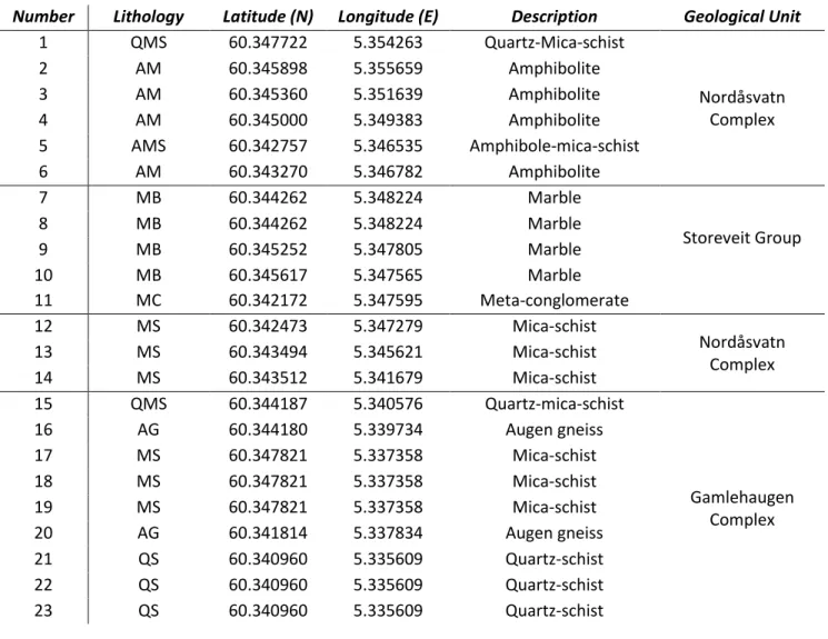
Table 1 List of the collected samples. Acronyms: QMS (quartz-mica-schist); AM (amphibolite); AMS 122
(amphibolite-mica-schist); MB (marble); MS (mica-schist); AG (augen gneiss); QS (quartz-schist). 123
Number Lithology Latitude (N) Longitude (E) Description Geological Unit
1 QMS 60.347722 5.354263 Quartz-Mica-schist Nordåsvatn Complex 2 AM 60.345898 5.355659 Amphibolite 3 AM 60.345360 5.351639 Amphibolite 4 AM 60.345000 5.349383 Amphibolite 5 AMS 60.342757 5.346535 Amphibole-mica-schist 6 AM 60.343270 5.346782 Amphibolite 7 MB 60.344262 5.348224 Marble Storeveit Group 8 MB 60.344262 5.348224 Marble 9 MB 60.345252 5.347805 Marble 10 MB 60.345617 5.347565 Marble 11 MC 60.342172 5.347595 Meta-conglomerate 12 MS 60.342473 5.347279 Mica-schist Nordåsvatn Complex 13 MS 60.343494 5.345621 Mica-schist 14 MS 60.343512 5.341679 Mica-schist 15 QMS 60.344187 5.340576 Quartz-mica-schist Gamlehaugen Complex 16 AG 60.344180 5.339734 Augen gneiss 17 MS 60.347821 5.337358 Mica-schist 18 MS 60.347821 5.337358 Mica-schist 19 MS 60.347821 5.337358 Mica-schist 20 AG 60.341814 5.337834 Augen gneiss 21 QS 60.340960 5.335609 Quartz-schist 22 QS 60.340960 5.335609 Quartz-schist 23 QS 60.340960 5.335609 Quartz-schist 124
Samples locations were selected according to the surface and depth distribution of the different 125
geological units and to the role of a specific lithotype unit played in the underground thermal and 126
hydraulic regime (Tab. 1). Nine samples belong to the Nordåsvatn Complex (the most representative 127
6
unit), nine to the Gamlehaugen Complex (expected to be the group of rocks with the greatest 128
thermal conductivity) and five specimens were collected in the Storetveit Group (the marble 129
formation expected to play a crucial role in the fluid circulation). Specimens 7-10 of the Storetveit 130
Group are marbles of the Marmorøyen Formation, which crops out in the study area (even if this 131
detail is not shown in Fig. 1, as outcrops are very small and difficult to map). 132
133
2.2 Thermal Conductivity Measurement Techniques
134
Four specific devices with different basic principles were used in order to compare the thermal 135
conductivity datasets and discuss the divergence in terms of fundamental theory behind each of 136
them, sample preparation and rock heterogeneity. Measurements were carried out by means of the 137
transient divided bar (TDB) (Pasquale et al. 2015), the transient line source (TLS) (Bristow et al. 138
1994), the optical scanning (OS) (Popov et al. 2016) and the guarded hot plate (GHP) (Filla 1997). 139
These methods are briefly described in the following together with the specific devices used to 140
perform the measurements. 141
2.2.1 Transient Divided Bar (TDB) 142
The device includes a stack of elements consisting of two copper blocks of known thermal capacity, 143
between which the studied rock specimen (cylindrical shape) is interposed. The upper block has the 144
same diameter of the specimen and acts as a heat source; the lower block is larger and acts as a 145
heat sink. When the room temperature T0 is attained, the lower copper block is plunged into a
146
thermostatic bath with temperature 10 to 15 °C lower than T0. The heat flowing through the sample
147
is equal to the heat adsorbed by the sink and the thermal conductivity can be found by monitoring 148
the temperature changes of the source and the sink (Pasquale et al. 2015). From Fourier’s postulate, 149
the amount of heat removed from the upper copper block Cu ΔTu in a given period of time ∆𝑡 =
150 𝑡2− 𝑡1 is: 151 152 𝐶𝑢
∙ ∆𝑇
𝑢=
𝜆𝑆 ℎ∫ (𝑇
𝑢− 𝑇
𝑙) 𝑑𝑡
𝑡2 𝑡1(1) 153 154
where Cu is the thermal capacity (J K-1) of the upper block at constant pressure, ΔTu (°C) the
155
temperature change of the upper block during a time step dt, λ (W m-1 K-1) the thermal conductivity
156
of the rock specimen, h (m) and S (m2) are the height and the cross-sectional area of the rock sample,
7
respectively, T is temperature and the suffixes u and l refer to upper and lower block. The change in 158
temperature is recorded by means of thermocouples connected to a digital acquisition system. 159
During the measurements, the temperature Tu and the difference Tu – Tl are recorded for a period
160
of at least 300 s. Thermal conductivity determinations are carried out at time steps of 10 s and 161
generally about 10 different time steps are analysed for each sample to obtain an average value. 162
Thermal conductivity can be obtained from: 163
164
𝜆 =
𝐶𝑢∙∆𝑇𝑢∙ℎ𝑆∙(𝑇̅̅̅̅−𝑇𝑢 ̅̅̅)∙∆𝑡𝑙
(2)
165
where 𝑇̅̅̅ − 𝑇𝑢 ̅𝑙 is the average difference between the values of Tu and Tl during the time step Δt.
166
Two correction factors are also taken into account. The first is related to the heat coming from the 167
specimen and therefore an effective heat capacity must be considered, that is the sum of Cu and
168
one third of the rock heat capacity (measured by means of a water calorimeter). The second 169
depends on the heat transfer from the surrounding environment to the upper block and can be 170
easily estimated by operating under steady state conditions, i.e. 2 hours after the beginning of the 171
test (Pasquale et al. 2015). The tests were carried out in a temperature-controlled environment at 172
20 °C and the thermal conductivity was determined with an accuracy of ± 5%. 173
2.2.2 Transient Line Source (TLS) 174
The line source method is based on the generation of heat at a constant rate by a heated wire. If 175
the line source is assumed to be infinitely long and infinitely thin, fully immersed in an infinite and 176
homogeneous medium, and a recording thermistor is placed in the same probe, the temperature 177
response, in a constant room temperature environment, can be described by: 178 179 𝑇2
− 𝑇
1= −
𝑞′ 4𝜋𝜆∙ ln(
𝑡2 𝑡2−𝑡1) (3)
180 181where q’ (W m-1) is the specific rate at which the heat is generated and T
1 and T2 (°C) are the
182
recorded temperatures at time steps t1 and t2 (s) respectively. This approximation of the general
183
heat transfer equation of an infinite line source allows for thermal conductivity measurements 184
with errors within ± 10% if the early time data (t < 200 s) are ignored and only the straight line in 185
a graph ΔT vs ln t is considered. 186
8
The apparatus adopted in this study is the commercial K2DPro Thermal Property Analyzer 187
(Decagon Devices) that fully complies with the standards ASTM D5334 and IEEE 442 (ASTM, 2014; 188
IEEE, 2003). A proprietary algorithm fits time and temperature data with exponential integral 189
functions using a non-linear least squares method. The single needle sensor RK-1 (length 6 cm, 190
diameter 3.9 mm), specific for hard rock samples, was used. A thin hole (4.5 mm in diameter) was 191
drilled into the sample in order to host the probe and alumina thermal grease (9 W m-1 K-1) was
192
applied to the probe in order to minimize the sensor/rock contact resistance. The measurements 193
were carried out in a controlled room temperature environment and the heating power was about 194
6.5 ± 0.5 W m-1 for all the whole set of samples. A 600 s measuring time was adopted (maximum
195
available) so that 300 s of heating and 300 s of cooling were recorded with a 10 s sampling interval. 196
At least 3 measurements were carried out on each sample and an average was taken. A time 197
interval of 15 min for each test was adopted in order to allow for the thermal re-equilibrium 198
between the sample and the probe. Before each triplet of measurements, a calibration was 199
performed with the verification standard provided and the calculated calibration factor was 200
applied to correct the thermal conductivity values (ASTM 2014). 201
2.2.3 Optical Scanning (OS) 202
The Optical Scanning is a precision non-contact method designed by Popov et al. (1999). It was 203
developed since the 80s by means of several comparisons with different techniques and calibrated 204
with a number of standard materials (Popov et al. 2016 and references therein). The measurement 205
procedure consists of scanning the sample of a surface with a focused movable heat source (electric 206
lamp) in combination with three infrared temperature sensors (Popov et al. 1999). The heat source 207
and sensors move with the same speed (controllable from 2 to 10 mm s-1) relative to the sample
208
and at a constant spacing xo among each other (adjustable from 20 to 100 mm). Rock samples are
209
placed on a platform in order to be scanned from below by the trolley containing the optical source 210
and the sensors. A synthetic black enamel is applied on the surface in order to neglect the influence 211
of optically transparent surfaces or different minerals’ reflectance. The technical parameters of the 212
apparatus adopted in this study are the ones described in Popov et al. 2016 for the Type 1. 213
The method is based on the heat conduction equation for a quasi-stationary field in a movable 214
coordinate system. The temperature rise induced in the sample and recorded along the scanning 215
line is related to the thermal conductivity as 216
𝑇
ℎ− 𝑇
𝑐=
𝑞2𝜋∙𝑥0∙𝜆 (4)
9
where Th and Tc (°C) are temperatures registered by the hot (after the heating source) and cold
218
(before) sensors, q (W) is the constant heating power and xo is the distance between the source and
219
the hot sensor. Since the temperature rise depends on both the heating power and the value of xo,
220
the measurements are always performed in comparison to standards of known thermal conductivity 221
(e.g. glasses, fused quartz, gabbro etc.). Standards are placed before and after the sample under 222
exam such that they are scanned with the same q and x0 and within the same room temperature.
223
In this study, an OS apparatus designed by Lippman and Rauen GbR was used. For all the 224
measurements q was set to about 17 W (20% of the maximum power) with a scanning velocity of 5 225
mm s-1 and x
0 = 50 mm. The standards adopted were homogeneous gabbro samples (provided by
226
the company) with thermal conductivity of 2.37 W m-1 K-1 and the measurements were performed
227
in a controlled temperature environment at around 20 °C. Three runs were carried out per each 228
sample’s scanning line and an average was taken. The accuracy certified by the company is ± 3%. In 229
case of a sample with a clear two-dimensional anisotropy (e.g. schists), the principal values of the 230
conductivity were determined from two non-collinear scanning lines performed on one face not 231
parallel to the foliation as suggested by Popov et al. 2016. This was done for all the samples in order 232
to check a possible thermal anisotropy even where a clear textural anisotropy was not present (e.g. 233
marbles). An anisotropy factor KT = λpar/λper was then calculated and the sample was considered
234
thermally homogeneous only in case of KT < 1.1.
235
2.2.4 Guarded Hot Plate (GHP) 236
The guarded hot plate or heat flow meter is a stationary technique based on standards ASTM C177 237
(2013) and ASTM C518 (2017) that also allows measuring thermal conductivity of semiconductors 238
at high temperatures (Filla 1997). A steady state one-dimensional heat flow is applied through a 239
specimen by two parallel plates guarded at different constant temperatures, while the whole stack 240
is insulated to avoid side heat losses. Temperature and heat flow are continuously registered on 241
both plates throughout the test by means of thermocouples and transducers, while an axial load is 242
provided to minimize the thermal contact resistance. 243
The apparatus adopted in this study is the commercial device Fox50 (LaserComp Inc., 2001-2004). 244
It can measure the thermal conductivity of cylindrical shaped samples, with diameters of 245
25 ÷ 61 mm and maximum thickness of 25 mm, in the range -5 ÷ 185 °C (Raymond et al. 2017). 246
Proprietary heat flow transducers together with high accuracy (± 0.01 °C) type E thermocouples are 247
bonded and sealed to the surfaces of both plates. Guarded temperature on the heat source (upper 248
10
plate) and sink (lower) are provided by Peltier elements and a downward heat flow is generated 249
through the rock specimen. From the Fourier heat conduction law, the temperature gradient within 250
the sample is given by the difference between the cold and hot plate temperatures divided by the 251
sample thickness. However, for conductivity values > 0.2-0.3 W m-1 K-1 (basically all the rocks and
252
minerals), the temperatures on the sample surfaces are different from the plates because the 253
thermal contact resistance is not significantly smaller than the sample thermal resistance. 254
Therefore, the temperature difference between the upper and lower plates is given by: 255
∆𝑇
𝑝𝑙𝑎𝑡𝑒𝑠= 𝛿𝑇
𝑢+ ∆𝑇
𝑠𝑎𝑚𝑝𝑙𝑒+ 𝛿𝑇
𝑙 (5) 256where δTu and δTl (°C) are the temperature differences between upper plate and sample surface,
257
and between sample surface and lower plate, respectively. The contact thermal resistance R (m2 K
258 W-1) is: 259
𝑅 =
𝛿𝑇 𝑞′′(6) 260
where q’’ (W m-2) is the heat flow recorded through each plate. R depends on the type of material,
261
the interface pressure applied and the roughness of the sample. The electric signal Q (V) recorded 262
by the heat flow transducers is proportional to the heat flow q’’ through a calibration factor 263
Scal [W m-2 V-1] that is determined using standard materials with known thermal conductivity. Q,
264
which is recorded during the experiment, is related to the thermal conductivity as: 265
𝑄 =
𝑞′′ 𝑆𝑐𝑎𝑙=
∆𝑇𝑝𝑙𝑎𝑡𝑒𝑠 (∆𝑥 𝜆+2𝑅)∙𝑆𝑐𝑎𝑙 (7) 266where Δx is the thickness of the sample. The absolute accuracy of the device is ± 3% in the 267
conductivity range of 0.1 ÷ 10 W m-1 K-1. Silicon or glycerine paste or rubber pads of known thermal
268
resistance can be employed to smooth the problem of contact resistance. The measurements were 269
carried out at 20 °C with a ΔT = 10 °C between the upper (25 °C) and lower (15 °C) plate and the 270
average of 10 sets of measurements was taken as final value. 271
272
2.3 Sample preparation
273
The whole sample collection was divided into two main datasets: dataset1 and dataset2. Dataset1 274
included all the 23 rock samples while dataset2 represents a subset of dataset1, namely nine 275
representative samples. Regarding thermal conductivity (see Section 2.2), most of samples of 276
11
dataset1 were analysed with two methods (OS and TLS), whereas dataset2 was additionally tested 277
with other two techniques (TDB and GHP). 278
Thermal conductivity in all 23 samples was studied in the two main directions, i.e. parallel (λpar) and
279
perpendicular (λper) to the main foliation. Five of the samples showed no clear foliation and KT < 1.1;
280
these are classified as thermally homogeneous and an average effective value was reported. This 281
procedure was adopted in both OS and TLS. For the measurements with OS, the samples were cut 282
according to the foliation in order to obtain two perpendicular polished surfaces upon which the 283
coating layer was applied. For the TLS analyses, previously cut and polished sample surfaces were 284
drilled with a 4 mm rotary hammer bit to host the RK-1 single needle sensor. Two perpendicular 285
drillings were performed in eleven out of twenty-three samples. Parallel and perpendicular 286
conductivity values were calculated with the same methodology adopted for OS (Popov et al. 2016) 287
and the anisotropy factor calculated. 288
Owing to issues related to obtain samples with the size and characteristics required by both TDB 289
and GHP, cylindrical rock specimens were prepared from samples of dataset2 by means of a 290
diamond-head corer and, through the use of a fine abrasive, both surfaces were rubbed down to 291
get flat (within 0.1 mm), parallel and smooth surfaces (within 0.03 mm). Finally, the obtained core 292
specimens had cylindrical shape, 25 ± 0.1 mm in diameter and 20 ± 0.5 mm in thickness. To improve 293
the contact between rock specimen and the blocks (TDB) and plates (GHP), a film of silicone paste 294
of about 0.1 mm was smeared on both samples surfaces. 295
Samples for OS and TLS are relatively easy to prepare, requiring a cut and painted surface (OS) or a 296
drilled hole (TLS). In contrast TDB and GHP require core drilling followed by precision grinding, 297
making their preparation critical to the success of the analysis. 298
299
2.4 Compressional wave velocity and density
300
The compressional wave velocity test is a non-destructive method based on the principle that pulse 301
velocity of ultrasound waves, propagating through a solid material, depends on the density and the 302
elastic properties of that material (Al-Khafaji and Purnell 2016). The commercial device PUNDIT Lab 303
(by Proceq Switzerland) was used in this study. The apparatus is coupled with a pair of transducers 304
that transmit and receive waves with a central frequency of 54 kHz, working on ASTM D2845 (2008) 305
procedure. The tests were performed on the samples as analysed by the OS technique, as flat 306
surfaces are necessary to make good contact between the specimen and the transducers. On each 307
12
sample, 25-30 measurements were carried out to get accurate results and the average between 308
these acquisitions was calculated. 309
Density was obtained by weighing the samples after water saturation under vacuum and measuring 310
their volume through immersion in water. Samples were then oven-dried at 70 °C for one day in 311
order to obtain the dry mass and to infer porosity. All the samples denoted negligible porosity (< 3%) 312
and thus water content was assumed to be of negligible importance on the measurements of petro-313 physical properties. 314 315 2.5 Mineralogical composition (XRD) 316
The mineralogical composition of the samples of dataset2 was investigated by means of powder 317
X-Ray diffraction (XRD) on crystalline samples. The measurements were performed with the Philips 318
X’Pert-Pro device (Malvern Panalytical ©2018) consisting of a Bragg-Brentano geometry and 319
equipped with a stationary, centrally placed, X-ray tube. The tube was operated using a CuKα 320
radiation at 40 mA, 40 kV and 1.5417 Å. Spectra were recorded in the 2θ range 5-70° with a 15 s 321
counting time and 0.008° 2θ step. 322
A qualitative analysis was firstly performed, distinguishing between two defined phase structures 323
of calcite and quartz present in each sample. The peak shape was modelled with a Pseudo-Voigt 324
function of which, the FWHM (Full Width of Half Maximum), was refined as a function of 2θ taking 325
into account both Gaussian and Lorentzian broadening. The refinement was carried out in 326
particular in the space group R-3c (calcite), P3221 (quartz).
327
In order to get an alternative estimate of the accuracy of the refined structural data, a comparison 328
among the set of structural parameters obtained using different refinement strategies on the same 329
diffraction data was carried out. These comparisons show that realistic estimates of the error bars 330
are ± 0.001 Å for the cell parameters. The error in the estimation of the phase content is ± 1% wt. 331 332 3. RESULTS 333 3.1 Dataset1 334
The bulk thermal conductivity values of dataset1 were measured by means of OS in the University 335
of Bergen’s laboratory (Tab. 2) and with TLS in the University of Torino’s laboratory (Tab. 3). The 336
samples coded B (e.g. 1_B) indicate that the specific rock specimens were measured in Bergen only; 337
those coded T (e.g. 1_T) indicate that they were analysed in Torino only; when the specimen is called 338
13
BT (e.g. 4_BT) means that the same rock specimen was measured by both techniques. This should 339
warn the reader that differences between 1_B and 1_T can even be related to the sample 340
heterogeneity and not only to the adopted techniques. Some samples (3_T, 9_BT, 13_BT, 17_BT, 341
18_BT, 19_BT) broke during preparation and it was not possible to analyse neither thermal 342
conductivity with TLS or OS, nor sonic velocity. 343
The standard deviations reported for OS are related to the values measured along the scanning lines 344
and thus due to the intrinsic heterogeneity of the rock samples. These cannot be compared to the 345
standard deviations of the TLS, which relate to the repeatability and precision of the KD2 Pro. The 346
standard deviations of the effective thermal conductivity (three runs along each scanning line) 347
measured with the OS were ± 0.7% on average, with a maximum of ± 1.6% and a minimum of ± 348
0.1%. OS and TLS bulk thermal conductivity was calculated as a geometric average between parallel 349
and perpendicular values. KT refers to the anisotropy factor given by the parallel to perpendicular
350
values ratio. 351
Mica-schists and amphibolites of the Nordåsvatn Complex show significant thermal anisotropy, with 352
parallel values higher than perpendicular ones by 50% in OS and 46% in TLS data. The marbles of 353
the Storeveit Group present an isotropic nature as expected, with anisotropy factor always smaller 354
than 1.1. The Gamlehaugen Complex shows clear thermal anisotropy in the quartz-schists and 355
quartz-mica-schists (KT > 1.2), in contrast to the general isotropic texture of both augen and
356
mylonitic gneisses (KT < 1.1). In absolute terms, the whole dataset is rather homogeneous, a bit
357
surprising given the presence of high quartz-content lithotypes. Low values of quartz-schists 21, 22 358
and 23 can be explained by abundant presence of muscovite, which presents strong anisotropy in 359
thermal conductivity (0.6 W m-1 K-1 perpendicular, 3.9 W m-1 K-1 parallel; Clauser and Huenges
360
1995). The OS average thermal conductivity is 2.75 W m-1 K-1 with a standard deviation of 0.29; TLS
361
data records an average conductivity of 2.18 W m-1 K-1 with a minimum of 1.37 and maximum of
362
3.16 (standard deviation 0.51). 363
364
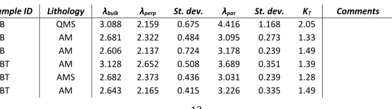
Table 2 Thermal conductivity λ (W m-1 K-1) and anisotropy factor K
T of dataset1 measured by means of OS.
365
Sample ID Lithology λbulk λperp St. dev. λpar St. dev. KT Comments
1_B QMS 3.088 2.159 0.675 4.416 1.168 2.05 2_B AM 2.681 2.322 0.484 3.095 0.273 1.33 3_B AM 2.606 2.137 0.724 3.178 0.239 1.49 4_BT AM 3.128 2.652 0.508 3.689 0.351 1.39 5_BT AMS 2.682 2.373 0.436 3.031 0.239 1.28 6_BT AM 2.643 2.165 0.415 3.226 0.335 1.49
14 7_BT MB 2.934 / / 2.934 0.174 / isotropic 8_BT MB 2.854 / / 2.854 0.128 / isotropic 9_BT MB 2.778 2.671 0.415 2.889 0.125 1.08 10_BT MB 2.995 2.913 0.621 3.079 0.194 1.06 11_BT MC 2.328 1.888 0.867 2.870 0.552 1.52 12_BT MS 2.826 2.461 0.470 3.246 0.199 1.32 13_BT MS 2.332 1.620 0.976 3.356 1.447 2.07 14_B MS 2.423 2.228 0.391 2.636 0.290 1.18 15_B QMS 3.333 3.233 0.540 3.437 0.169 1.06 16_B AG 2.955 / / 2.955 0.189 / isotropic 17_BT MS 2.275 2.069 0.269 2.500 0.379 1.21 18_BT MS 2.906 / / 2.906 0.862 / isotropic 20_B AG 2.946 2.924 0.645 2.969 0.299 1.02 21_B QS 2.677 2.286 1.288 3.134 0.563 1.37 22_BT QS 2.842 2.300 0.884 3.511 0.308 1.53 23_B QS 2.301 2.103 0.425 2.518 0.280 1.20 366
Table 3 Thermal conductivity λ (W m-1 K-1) values and anisotropy factor K
T obtained with TLS.
367
Sample ID Lithology λbulk λperp St. dev. λpar St. dev. KT Comments
1_T QMS 1.367 1.006 0.060 1.859 0.074 1.85
2_T AM 2.422 2.745 0.072 2.137 0.104 0.78
4_BT * AM 2.743 / / 2.743 0.097 / only perp. drilling possible
5_BT * AMS 2.266 / / 2.266 0.045 / only perp. drilling possible
6_BT AM 1.911 1.613 0.035 2.263 0.107 1.40
7_BT MB 2.518 / / 2.518 0.127 / isotropic
8_BT MB 2.448 / / 2.448 0.175 / isotropic
10_BT ** MB 2.317 2.317 0.137 / / / only par. drilling possible
11_BT MC 1.797 1.291 0.096 2.501 0.165 1.94 12_BT MS 2.042 1.538 0.130 2.712 0.055 1.76 14_T MS 1.773 1.454 0.084 2.162 0.067 1.49 15_T QMS 3.023 2.513 0.184 3.636 0.095 1.45 16_T AG 3.155 / / 3.156 0.456 / isotropic 20_T AG 2.066 1.856 0.073 2.299 0.146 1.24
21_T * QS 1.426 / / 1.426 0.034 / only perp. drilling possible
22_BT QS 2.175 1.779 0.088 2.659 0.152 1.50
23_T QS 1.621 1.699 0.038 1.547 0.042 0.91
* parallel value; ** perpendicular value 368
369
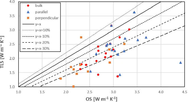
Comparing the results of the different techniques, we observe a general underestimation of TLS 370
with respect to OS, both for the bulk conductivity and λpar and λper (Fig. 2). TLS underestimates
371
thermal conductivity with respect to OS, with a maximum difference of 56% (sample 1) in the bulk 372
value. Generally, the higher biases occur in the parallel analyses (58%) than in those perpendicular 373
15
(54%). By taking OS as a reference, 68% of the TLS results underestimate the thermal conductivity 374
of the rock samples analysed by a minimum of 10% to a maximum of 30%; for the 24%, the 375
underestimate is more than 30% and only few outliers (8%) overestimate it. A significant difference 376
among bulk, parallel and perpendicular values is not clearly evident in Figure 2. If only the BT 377
samples are taken into consideration, the underestimate of TLS with respect to OS is on average 378
20.1%, 20.3% and 27.5% for bulk, parallel and perpendicular values respectively, with a minimum 379
of 12.3% (4_BT bulk) and maximum of 37.5% (12_BT perpendicular). 380
381
382
Figure 2 Comparison between OS and TLS bulk, parallel and perpendicular values of thermal conductivity 383
384
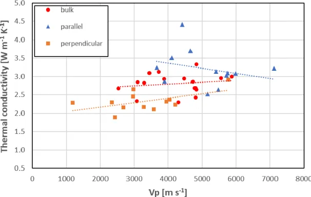
No clear direct correlation between bulk thermal conductivity (from OS technique) and P-wave 385
velocity is observed in dataset1 (Fig. 3). Mielke et al. (2017) also showed that low-porosity rocks, as 386
those investigated in this paper, present weak correlations. It is nevertheless interesting to note the 387
contrast between properties when considered parallel and perpendicular to the main rock foliation. 388
Perpendicular conductivity values grow with increasing perpendicular sonic velocity, while parallel 389
values exhibit an inverse trend. Therefore, it is shown that only along the direction perpendicular to 390
foliation heat and P-waves propagation in the medium follow similar patterns. Conversely, when 391
analysing the sample along the main foliation, propagation paths might not be necessarily the same. 392
Unfortunately, due to the heterogeneity of the collection and the limited number of samples, this 393
cannot be related to specific rock features. It would be necessary to investigate further, but this 394
goes beyond the purpose of the present paper. When comparing the anisotropy factors (Tab. 4), 395
16
the data are quite similar, with eight out of twelve samples showing a KS/KT ratio within the 0.85 ÷
396
1.15 range (i.e. 15% bias) and the best results occurring in the BT samples (same specimen analysed 397
by both techniques). 398
399
400
Figure 3 Relationship between thermal conductivity (OS technique) and P-wave velocity. 401
402
Table 4 P-wave velocity Vp (m s-1), sonic (K
S) and thermal anisotropy (KT from OS) of dataset1. N is the
403
number of measurements. 404
Sample ID Lithology Vpbulk Vpperp St.
dev. N Vppar St. dev. N KS KT KS / KT 1_T / 1_B MS 3448 2691 45 27 4418 353 28 1.64 2.05 0.80 2_T / 2_B AM 4769 3953 154 27 5753 165 27 1.46 1.33 1.09 4_BT AM 3727 2978 114 27 4664 136 27 1.57 1.39 1.13 5_BT AMS 4805 4038 124 28 5719 171 27 1.42 1.28 1.11 6_BT AM 4836 3284 92 28 7123 296 27 2.17 1.49 1.46 10_BT MB 5877 5774 274 26 5982 107 27 1.04 1.06 0.98 11_BT MC 3082 2435 27 26 3901 118 26 1.60 1.52 1.05 12_BT MS 3295 2963 73 26 3664 58 26 1.24 1.32 0.94 14_T / 14 B MS 4804 4209 127 26 5483 226 27 1.30 1.18 1.10 21_T / 21_B QS 2533 1187 57 27 5407 209 27 4.55 1.37 3.32 22_BT QS 3099 2343 37 27 4100 123 27 1.75 1.53 1.15 23_T / 23_B QS 4301 3577 128 27 5172 81 27 1.45 1.20 1.21 405 3.2 Dataset2 406
17
Dataset2 comprised nine of the dataset1 samples further studied using GHP and TLS. Of the nine 407
specimens, 3 are perpendicular and one is parallel to the main foliation; the rest are from isotropic 408
samples. Cylindrical shape specimens were obtained from the samples analysed with the OS and 409
TLS techniques (samples BT) or by the TLS only (samples T). 410
411
Table 5 Comparison of thermal conductivity results of dataset2 measured with the four techniques (see 412
text); the accuracy of each technique is in brackets. Last column reports average values from literature 413
(aČermák and Rybach 1982; bKukkonen and Peltoniemi 1998; cDi Sipio et al. 2014; dEppelbaum et al. 2014;
414
eRamstadt et al. 2015; fMielke et al. 2017).
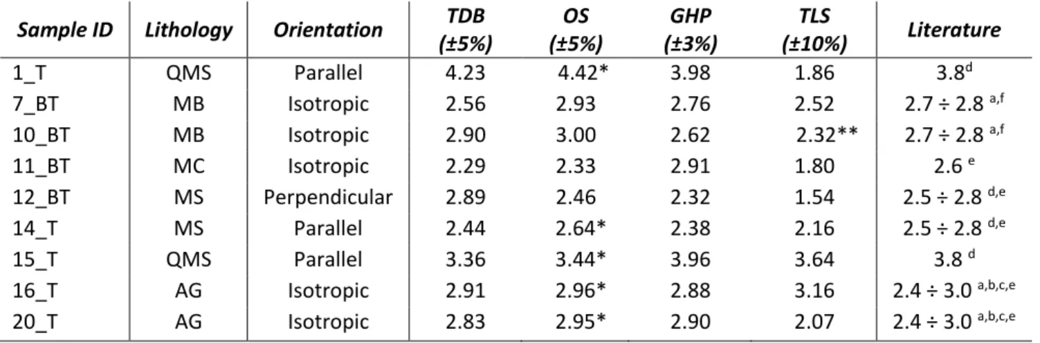
415
Sample ID Lithology Orientation TDB
(±5%) OS (±5%) GHP (±3%) TLS (±10%) Literature 1_T QMS Parallel 4.23 4.42* 3.98 1.86 3.8d 7_BT MB Isotropic 2.56 2.93 2.76 2.52 2.7 ÷ 2.8 a,f 10_BT MB Isotropic 2.90 3.00 2.62 2.32** 2.7 ÷ 2.8 a,f 11_BT MC Isotropic 2.29 2.33 2.91 1.80 2.6 e 12_BT MS Perpendicular 2.89 2.46 2.32 1.54 2.5 ÷ 2.8 d,e 14_T MS Parallel 2.44 2.64* 2.38 2.16 2.5 ÷ 2.8 d,e 15_T QMS Parallel 3.36 3.44* 3.96 3.64 3.8 d 16_T AG Isotropic 2.91 2.96* 2.88 3.16 2.4 ÷ 3.0 a,b,c,e 20_T AG Isotropic 2.83 2.95* 2.90 2.07 2.4 ÷ 3.0 a,b,c,e
* the B specimen was measured; ** perpendicular value 416
417
The results are consistent with average values in literature (Tab. 5). The analysis of dataset2 418
confirms that TLS underestimates thermal conductivity with respect to TDB (-26% on average) and 419
GHP (-24% on average), with a maximum of more than 50% in sample 1_T, which is highly 420
anisotropic. It is worth stressing that in four samples (7_BT, 14_T, 15_T and 16_T) the bias with GHP 421
is within the 10% accuracy expected for the TLS device. In particular, in the very homogeneous and 422
isotropic augen gneiss 16_T, TLS registers a thermal conductivity higher than TDB, OS and GHP by 423
9%, 7% and 10% respectively. A conductivity greater than TDB (8%) and OS (6%) is also given by TLS 424
in the same lithology of 15_T (Fig. 4). 425
On the contrary, a good general agreement between OS, TDB and GHP is observed (Fig. 5): a 7-8% 426
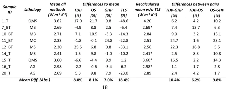
divergence from the overall mean is registered compared to an 18% average bias recorded by TLS. 427
In the five samples in which the TLS bias is greater than the accuracy of the devices used for the 428
analyses (error bars do not overlap), that value was discarded and a new average calculated (Tab. 429
6). The new values were then adopted to compare the different techniques. TDB and OS show an
430
average divergence of 6% with maximum of 16.8% and 13.7% in 12_BT and 7_BT respectively. 431
18
Moreover, TDB and OS are within 5% in six out of nine samples. Comparisons between GHP and OS, 432
and GHP and TDB have worse accordance, with average 9.8% and 10.4% respectively, and only in 433
two and three cases better than 5%. The greatest biases are observed in BT samples, wherein the 434
same specimen was analysed by means of the three techniques: in particular, the largest deviations 435
(24.7% and 22.3%) were obtained between TDB and GHP, which used the same core sample. The 436
discrepancy could be attributed to the difference between static and transient analyses: in three 437
out of nine samples (11_BT, 12_BT and 15_T), TDB and GHP error bars do not overlap. 438
439
440
Figure 4 Thermal conductivity results of dataset2. 441
442 443 444
Table 6 Comparison of thermal conductivity results for dataset2. 445 Sample ID Lithology Mean all methods (W m-1 K-1)
Differences to mean Recalculated
mean w/o TLS (W m-1 K-1)
Differences between pairs TDB [%] OS [%] GHP [%] TLS [%] TDB-GHP [%] TDB-OS [%] OS-GHP [%] 1_T QMS 3.62 17.0 21.7 9.8 -48.6 4.20 6.2 4.2 10.2 7_BT MB 2.69 -4.9 8.8 2.5 -6.4 2.69* 7.4 13.7 6.3 10_BT MB 2.71 7.1 10.5 -3.3 -14.3 2.84 9.9 3.2 13.1 11_BT MC 2.33 -1.8 -0.1 24.8 -22.8 2.51 24.7 1.6 23.1 12_BT MS 2.30 25.5 6.8 0.8 -33.1 2.56 22.3 16.8 5.5 14_T MS 2.41 1.5 9.8 -1.0 -10.2 2.41* 2.5 8.3 10.8 15_T QMS 3.60 -6.6 -4.4 9.9 1.2 3.60* 16.5 2.2 14.3 16_T AG 2.98 -2.2 -0.6 -3.4 6.2 2.98* 1.1 1.7 2.8 20_T AG 2.69 5.3 9.8 7.9 -23.0 2.89 2.4 4.2 1.7
19 * value of the first column
446 447
448
Figure 5 Comparison of conductivity measurement techniques for dataset2.
449 450
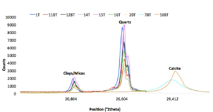
451
Figure 6 XRD results of the main mineral groups of dataset2 samples. 452
453
XRD analyses show the bulk mineralogy of the samples, entirely quartz and clay/mica except two 454
with carbonate (Fig. 6). These analyses were performed because many of the samples have a 455
microcrystalline structure, so the recognition of the mineral phases with optical techniques is often 456
difficult and in many cases not useful from a quantitative point of view. Quartz and micas are the 457
main mineral phases of the mica-schists and gneisses, while calcite is predominant in the marbles 458
20
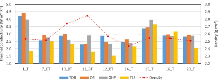
(samples 10_BT and 7_BT; Fig. 6). As expected, Table 6 shows that higher quartz content 459
corresponds to higher thermal conductivity. For example, the quartz-mica schist samples 1_T and 460
15_T have mean conductivities of 4.2 and 3.6 W m-1 K-1 respectively. These samples also have low
461
density, consistent with the low relative density of quartz and mica (Fig. 7). The high content of 462
micas (likely muscovite and biotite) might mask significant differences between silicate and 463
carbonate samples, given that calcite thermal conductivity (3.2÷3.6 W m-1 K-1; Clauser and Huenges
464
1995; Andolfsson 2013) is higher than micas (2.0÷2.3 W m-1 K-1; Clauser and Huenges 1995). In
465
samples with calcite or likely other dense mineral phases (e.g. olivine), not clearly detected in the 466
XRD study, we noticed lower thermal conductivity which is accompanied by higher density values 467
(e.g. 10_BT and 11_BT, Fig. 7). The thermal conductivity and density of 10_BT is consistent with 468
isotropic marble. 11_BT is characterized by the highest density and lowest conductivity. Its density 469
and thermal conductivity are consistent with the facies description of clasts of trondjemite, 470
epidosite and amphibolite (Fossen 1989). Density ranges for these rocks are: trondjemite 2.7, 471
epidosite 2.8÷3.0 and amphibolite 2.9÷3.1 g cm-3; thermal conductivity: trondjemite 1.8÷2.6,
472
epidosite 2.4÷4.5 and amphibolite 2.2÷2.9 W m-1 K-1 (Popov et al. 1999; Miao et al. 2014, Merriman
473
et al. 2013). The XRD shows relatively low peaks for quartz and mica, and, at slightly lower 2-theta 474
than quartz, some additional low peaks not present in the other samples (Fig. 6). 475
476
Figure 7 Comparison between thermal conductivity and density in dataset2. 477
478
4. DISCUSSION
479
Among the techniques used for the thermal conductivity analyses of our samples, it is reported in 480
the literature that TLS is a valid method to measure highly porous, soft materials (e.g. Di Sipio et al. 481
2014), but with hard materials the results may often be affected by large biases. In our analyses, 482
particular care has been adopted in sample preparation. Each sample was previously prepared with 483
21
two parallel surfaces in order to have a 90° ± 5° angle with the drill bit; a drill press was used to drill 484
the sample to assure a precise perpendicular drilling; water was constantly poured in to safeguard 485
the widia-diamond bit and facilitate the exit of drill cutting; the hole was cleaned up by removing 486
dust and cuttings with compressed air after the end of drilling; the probe and the inner hole were 487
carefully coated with thermal grease; finally, the probe was inserted slowly to allow trapped air to 488
escape. 489
Despite the careful sample preparation, the TLS systematically showed low values with respect to 490
the other three techniques. TLS gave lower conductivity than OS (more than 90% of samples in 491
dataset1) and GHP and TDB (more than 65% in dataset2). Anisotropy seems to have some influence, 492
the average bias being 14% in isotropic against 27% in anisotropic rocks, even if isotropic samples 493
10_BT and 20_T showed biases of 23 and 30%. By increasing the TLS values by 20%, more than half 494
of the samples would be within 10% of the OS value (dataset1). However, in dataset2 this would 495
cause severe overestimation for samples 7_BT, 15_T and 16_T. In summary, we infer the “high” 496
values are correct, and attribute the “low” values to problems with deficiencies in the sample 497
preparation for TLS measurements. Clearly, TLS strongly depends on sample preparation and 498
heterogeneity and anisotropy of the rock. Isotropic, homogeneous and competent (weathered 499
samples could break during preparation) lithotypes can limit the bias to < 10% if care is taken in the 500
measurement procedure above explained. For anisotropic and highly heterogeneous rocks, and 501
weak or weathered samples, the other methods are preferable to avoid significant underestimation 502
of the actual thermal conductivity. 503
Even though the GHP and the TDB methods are similar in sample preparation and precautions to 504
limit the contact resistance were adopted (in two cases, 11_BT and 12_BT, the specimens were even 505
the same), the results were similar in samples 7_BT, 16_T and 20_T, but significantly different in 506
samples 10_BT, 11_BT, 12_BT and 15_T. A systematic explanation for the variation in results is not 507
evident. Only minor influence on the results was found for the heterogeneity and anisotropy of the 508
samples. It is nevertheless evident that the core preparation is crucial to get reliable results; but it 509
also seems that other factors are important, such as the quality of the measuring stack (contact 510
between plates/blocks and sample, accuracy of temperature sensors/heat flow meters) and the 511
employment of standards (TDB) rather than previously obtained calibration curves (GHP). 512
Smaller biases were obtained between GHP and OS, and TDB and OS, with the TDB-OS differences 513
being consistently smaller than the others. Differences with OS are also related to the different 514
measuring procedures. The OS scans the entire sample while the other techniques give instead more 515
22
localized information. Thus, the OS can thoroughly characterize a rock sample with information 516
about heterogeneity and thermal anisotropy in an easier way in comparison to the other three 517
techniques. Another advantage of the OS is the simple sample preparation. Last but not least, the 518
problem of thermal contact resistance is bypassed. On the other hand, samples for OS analysis must 519
be big enough to neglect boundary effects (Popov et al. 2016), even if the energy input (heat and 520
speed) can be varied accordingly. 521
Finally, it is important to stress that OS is the fastest way to analyse thermal conductivity, not only 522
in terms of single measurement (1-2 min against 5-8 min with TDB and 60-70 min with GHP), but 523
also for the simplest sample preparation. The OS seems to be the best with friable and weathered 524
samples since there is no contact and only a flat surface is required, but micro-cracks are still a 525
problem. Nevertheless, if the sample is competent enough, drilling several cores with different 526
orientations allows evaluating thermal anisotropy also with GHP or TDB. 527
Bulk thermal conductivity and sonic velocity values did not show a clear direct correlation in the 528
collections under study, herein attributed to the low porosity of the samples (Mielke et al. 2017). 529
This could be related to the opposite trends observed in the parallel and perpendicular analyses, 530
that show an inverse and a direct relationship respectively. In the authors’ knowledge, this has not 531
been reported in literature so far and deserves to be investigated further. 532
A clearly defined correlation between thermal conductivity and density was not recorded. However, 533
in quartz-rich samples we observed high thermal conductivity and low density as also observed by 534
Pasquale et al. (2015). On the contrary, in calcite-rich samples we noticed lower thermal 535
conductivity not related to a well-defined density value. The presence of micas is likely to mask 536
major differences between silicate and carbonate samples. 537
538
5. CONCLUSIONS
539
A comparison among four different laboratory methodologies to analyse the rock thermal 540
conductivity was carried out. Steady state (GHP) and transient (TLS, TDB, OS) methods were adopted 541
and results compared to highlight qualities and flaws of the different techniques. Moreover, 542
compressional wave velocities, density and mineral composition were investigated. The results of 543
this study are preparatory for future activities that will encompass the set-up of numerical modelling 544
of the underground thermal structure of the BHE field in Bergen. 545
Among the four methods for measuring thermal conductivity, even if steady state techniques are 546
expected to be more accurate, our results indicate that TDB and OS give more congruent results. 547
23
TLS, instead, systematically underestimates thermal conductivity in the investigated samples, 548
confirming that it is hardly applicable to hard rocks. Due to heterogeneity, anisotropy and 549
mechanical properties of the rocks, the use of at least two different techniques seems 550
recommendable in investigations on rock thermal properties. An uncertainty of 5 to 10% is the best 551
that one can expect even in good-quality and homogeneous samples. Geothermal modelling often 552
relies on values of thermal conductivity without well-defined uncertainty boundaries. The inclusion 553
of this uncertainty may increase the reliability of estimations. 554
555
Acknowledgments
556
The authors would like to thank the laboratory of the University of Bergen, in particular Niels Bo 557
Jensen, for carrying out measurements and processing the data with the TCS. Giorgia Confalonieri 558
and Alessandro Pavese, are also warmly thanked for the XRD analyses. The authors are extremely 559
grateful to Jasmin Raymond for the use of the GHP in the Geothermal Open Lab at the Institut 560
national de la recherche scientifique of Québec, Canada. 561
562
Author Contributions
563
N.G. collected the samples and took care of the samples preparation for OS and TLS, measurements 564
and data processing of thermal conductivity with TLS; he also performed P-wave analyses and 565
processed the data. J.C. prepared the samples, carried out analyses and processed the data of TDB 566
and GHP; she also took care of XRD processing and density analyses. N.G. and J.C. wrote together 567
the original draft paper, finalizing figures and tables. W.H.W. and G.M. conceptualized the original 568
idea of the study, and together with M.V. advised on the rigorous experimental analyses and revised 569 the manuscript. 570 571 References 572 573
Alishaev MG, Abdulagatov IM, Abdulagatova ZZ (2012) Effective thermal conductivity of fluid-574
saturated rocks. Experiment and modeling. Eng Geol 135-136:24-39. 575
Al-Khafaji S, Purnell P (2016) Effect of coupling media on ultrasonic pulse velocity in concrete: a 576
preliminary investigation. Int J Civ Env Eng 10:118-121. 577
Andolfsson T (2013) Analyses of thermal conductivity from mineral composition and analyses by use 578
of Thermal Conductivity Scanner: A study of thermal properties in Scanian rock types. 579
Dissertation, Lund University. 580
24
ASTM C177 (2013) Standard test method for steady-state heat flux measurements and thermal 581
transmission properties by means of the guarded-hot-plate apparatus. ASTM International, 582
West Conshohocken, PA, doi: 10.1520/C0177-13. 583
ASTM D5334 (2014) Standard test method for determination of thermal conductivity of soil and soft 584
rock by thermal needle probe procedure. ASTM International, West Conshohocken, PA, doi: 585
10.1520/D5334-14. 586
ASTM C518 (2017) Standard test method for steady-state thermal transmission properties by means 587
of the heat flow meter apparatus. ASTM International, West Conshohocken, PA, doi: 588
10.1520/C0518-17. 589
ASTM D2845 (2008) Standard test method for laboratory determination of pulse velocities and 590
ultrasonic elastic constants of rock. ASTM International, West Conshohocken, PA, doi: 591
10.1520/D2845-08. 592
Bristow KL, White RD, Kluitenberg GJ (1994) Comparison of single and dual probes for measuring 593
soil thermal properties with transient heating. Austr J Soil Res 32:447-464. 594
Cabeza LF (2015) Advances in thermal energy storage systems – methods and applications. 595
Woodhead Publishing, Cambridge, UK. 596
Čermák VL, Rybach L (1982) Thermal conductivity and specific heat of minerals and rocks. In: 597
Angenheister G (ed) Numerical Data and Functional Relationships in Science and Technology, 598
New Series, Group V (Geophysics and Space Research), Vol. 1a (Physical Properties of Rocks), 599
Springer, Berlin, pp 305-343. 600
Clauser C, Huenges E (1995) Thermal conductivity of rocks and minerals. Rock physics & phase 601
relations: a handbook of physical constants, American Geophysical Union, pp 105-126. 602
Di Sipio E, Galgaro A, Destro E, Teza G, Chiesa S, Giaretta A, Manzella A (2014) Subsurface thermal 603
conductivity assessment in Calabria (southern Italy): a regional case study. Env Earth Sci 604
72:1383-1401. 605
Eppelbaum L, Kutasov I, Pilchin A (2014) Thermal properties of rocks and density of fluids. In: Applied 606
Geothermics. Springer, Berlin, pp 99-149. 607
Filla BJ (1997) A steady-state high-temperature apparatus for measuring thermal conductivity of 608
ceramics. Rev Sci Ins 68(7):2822-2829. 609
Fossen H (1989) Geology of the Minor Bergen Arc, West Norway. Norg Geol Unders Bull, 416:47-62. 610
Fossen H, Ragnhildstveit J (2008) Berggrunnskart 1115 I, Scale 1:50.000, Norge Geol Unders. 611
Fuchs S, Schütz F, Förster HJ, Förster A (2013) Evaluation of common mixing models for calculating 612
bulk thermal conductivity of sedimentary rocks: correction charts and new conversion 613
equations. Geoth 47:40-52. 614
Giordano N, Chicco J, Bastesen E, Wheeler WH, Mandrone G (2017) Thermo-hydraulic 615
characterization of a fractured shallow reservoir in Bergen (Norway) to improve the efficiency 616
of a BHE field. European Geosciences Union, General Assembly, April 23-28, Wien, Austria, 617
EGU2017-18581. 618
25
Giordano N, Comina C, Mandrone G, Cagni A (2016) Borehole thermal energy storage (BTES). First 619
results from the injection phase of a living lab built up in unsaturated alluvial deposits (Torino, 620
IT). Ren En 86:993-1008. 621
IEEE Guide for Soil Thermal Resistivity Measurements (2003). IEEE Std 442-1981 1–16. 622
Kolderup CF, Kolderup NH (1940) Geology of the Bergen Arc System. Bergen Museums Skrifter, 20, 623
137 p. 624
Kukkonen IT, Peltoniemi S (1998) Relationships between thermal and other petrophysical 625
properties of rocks in Finland. Phys Chem Earth 23(3):341-349. 626
Lund JW, Boyd TL (2015) Direct utilization of geothermal energy 2015 worldwide review. 627
Proceedings World Geothermal Congress, n. 01000, April 19-25, Melbourne, Australia. 628
Merriman JD, Whittington AG, Hofmeister AM, Nabelek PI, Benn K (2013). Thermal transport 629
properties of major Archean rock types to high temperature and implications for cratonic 630
geotherms. Precambrian Res 233:358-372. 631
Miao SQ, Li HP, Chen G (2014). Temperature dependence of thermal diffusivity, specific heat 632
capacity, and thermal conductivity for several types of rocks. J Therm Anal Calorim 115(2): 1057-633
1063. 634
Midttømme K, Ramstad RK, Müller J (2015) Geothermal energy – Country update for Norway. 635
Proceedings World Geothermal Congress, n. 01071, April 19-25, Melbourne, Australia. 636
Mielke P, Bär K, Sass I (2017) Determining the relationship of thermal conductivity and 637
compressional wave velocity of common rock types as a basis for reservoir characterization. J 638
App Geophys 140:135-144. 639
Pasquale V, Verdoya M, Chiozzi P (2015) Measurements of rock thermal conductivity with a 640
Transient Divided Bar. Geoth, 53:183-189. 641
Popov YA, Beardsmore G, Clauser C, Roy S (2016) ISRM Suggested methods for determining thermal 642
properties of rocks from laboratory tests at atmospheric pressure. Rock Mechanics and Rock 643
Engineering 49:4179-4207. 644
Popov YA, Pribnow DFC, Sass JH, Williams CF, Burkhardt H (1999) Characterization of rock thermal 645
conductivity by high-resolution optical scanning. Geoth 28:253-276. 646
Ramstad RK, Midttømme K, Liebel TH, Frengstad BS, WIllemoes-Wissing B (2015) Thermal 647
conductivity map of the Oslo region based on thermal diffusivity measurements of rock core 648
samples. Bull Eng Geol Env 74:1275-1286. 649
Raymond J, Comeau F-A, Malo M, Blessent D, López Sánchez IJ (2017) The geothermal open 650
laboratory: a free space to measure thermal and hydraulic properties of geological materials. 651
IGCP636 Annual Meeting, Santiago de Chile, Chile, 1-3. 652
Yang H, Cui P, Fang Z, (2010) Vertical-borehole ground-coupled heat pumps: a review of models and 653
systems. App En 87:16-27. 654
Zhao D, Quian X, Gu X, Ayub Jajjia S, Yang R (2016) Measurement techniques for thermal 655
conductivity and interfacial thermal conductance of bulk and thin film materials. J Elect 656
Pack 138(4):040802. 657