Multivariable statistical analysis for enhancing performance indicators in direct contact membrane distillation
Bader Bin Ashoora, Adewale Giwab, Shadi W. Hasanc,*, Taha B.M.J. Ouardad, Adel Mhamdie
a-c
Department of Chemical Engineering, Khalifa University of Science and Technology, Masdar City Campus, P.O. Box 54224, Abu Dhabi, United Arab Emirates
d
Institut National de la Recherche Scientifique, Centre Eau Terre Environnement, Québec, G1K9A9, Canada
a,e
AVT-Process Systems Engineering, RWTH Aachen University, D-52056 Aachen, Germany.
a
[email protected]; [email protected]; c,*[email protected];
d
[email protected]; [email protected]; c,*+971 2 810 9237
Abstract
Orthogonal experimental design, correlation analysis and response surface charts were used to identify the parameters influencing the operational efficiency of direct contact membrane distillation (DCMD). The orthogonal array design method was used to optimize the number of experimental trials required for dependence analysis. The operating factors studied were hot feed properties (temperature, salinity, flowrate) and cold distillate characteristics (temperature, and flowrate). The impact of those factors on three DCMD performance indicators - cold distillate production rate, performance ratio and recovery ratio - was investigated. The most significant factors influencing each performance indicator were obtained from the quantitative values of main and interaction effects, and confirmed by using the Pearson product-moment correlation coefficients. The main effects of feed and distillate temperatures on the performance indicators were the greatest, indicating that the most significant factors were the feed and distillate temperatures. The maximum distillate production rate was obtained at feed and distillate temperatures of 90 and 15oC, respectively. The optimum recovery and performance ratios were obtained at a feed flowrate of 1.6 L/min but when feed temperature was kept at 70oC.
Keywords: Membrane distillation; orthogonal design; Pearson correlation; response surface analysis; desalination.
2 1. Introduction
The need for the provision of potable water is becoming increasingly crucial as a result of persistent rise in the world’s population [1,2]. Desalination of saline water and treatment of wastewater are two viable ways of producing fresh water for several applications [3–5]. Recently, several advancements have been made in the wastewater treatment sector in order to encourage water reuse and lessen the depletion rate of other water resources. These improvements have resulted in the production of high-quality effluents and less hazardous wastes [6–9]. However, in dry and arid locations such as the United Arab Emirates with burgeoning economy, the application of an inexhaustible feed water source (such as seawater) is imperative. The sustainability of continued desalination in these locations would depend largely on the development of desalination technologies that are simple and can be used for decentralized applications such as membrane distillation (MD) [10,11].
MD process integrates membrane and thermal desalination processes through which saline feed water is heated generating water vapor that passes through a hydrophobic membrane. The vapor obtained condenses on the opposite side of the membrane and is collected as cold distillate [10]. This process is driven by a difference in temperature between the membrane sides. In MD, three important processes occur: (i) evaporation of water from a hot saline feed; (ii) transportation of vapor through a porous membrane; and (iii) condensation of vapor to fresh distillate. The difference in temperature maintained across both sides of the membrane ensures the attainment of a vapor pressure difference [12]. Owing to the low surface energy of polymeric materials that are mostly used for MD membranes, only water vapor can pass through the membrane [13]. Several MD studies were demonstrated in laboratory scale or pilot systems [10,12,14–18]. Meanwhile, flat sheet direct contact membrane distillation (DCMD) configuration is the most widely and commercially used configuration in MD studies because of its simplicity to design and operate [18,19]. DCMD (like other MD configurations) permits the use of low grade heat for water desalination and membrane fouling is minimized as a result of the passage of vapor only through a DCMD membrane. However, values of water flux obtainable from DCMD, as reported in the literature, varied between low and in excess of 40 L/m2h (LMH) which means that for DCMD, it is not flux that is the greatest challenge, it is the specific energy utilization [13]. The goal of this work was to identify the control factors that critically influence the DCMD performance indicators. A standard orthogonal array experimental design was used to identify the optimal setting of control factors which will maximize the DCMD performance indicators. The control factors are those which can be easily manipulated under normal conditions. The orthogonal array design method was the factorial technique used to optimize the number of experimental trials required for this dependency analysis. The use of the mathematical models to determine the significant performance indicators would be inefficient and time-consuming because each parameter would be varied while other parameters or properties are kept constant.
3
Numerical modeling approach would be too costly since many experiments would be required for parameter estimation and model validation, depending on the incremental steps selected for each variable. However, the combination of orthogonal array design and response surface analysis is a non-mechanistic tool which contributed to the reduction of experimental trials required for this investigation. The orthogonal array experimental design helped to systematically determine factors that influence process variability.
Instead of having to test all possible combinations like the factorial design, the orthogonal arrays method evaluated the most significant combinations, whereby all variables were varied simultaneously in incremental steps or levels. Previous research efforts on the dependence of DCMD performance on operating conditions have been mainly directed towards the comparison of different membranes with different characteristics [20]. In addition, Alklaibi and Lior [21–23] attempted to evaluate the dependence of operating parameters such as feed/permeate temperatures and velocities on mass transfer resistances and thermal efficiency. For example, the physical domains influencing the mass transfer resistances of AGMD and DCMD were evaluated and compared by Alklaibi and Lior [21], using two-dimensional conjugate model that involves a simultaneous numerical solution of the momentum, energy and diffusion equations of the feed and cold solutions. It was found that the feed inlet temperature and air/vapor gap have the greatest influence on the mass transfer resistances and thermal efficiency of the AGMD. The feed and permeate velocities and the feed concentration have slight effects on the process performance. Also, it was observed from the solution of the two-dimensional conjugate problem that, while the thermal efficiency of AGMD is higher than that of DCMD by about 6%, the permeate flux of DCMD is higher than that of AGMD by about 2.3-fold and 4.8-fold when the feed inlet temperature was 80 and 40°C, respectively [22].
However, the numerical solutions of the models developed and reported in the works of Alklaibi and Lior were validated with experiments that employed a laboratory-scale experimental set-up. In addition, mathematical methods were used to predict the experimental results only. In this paper, a combination of mathematical and statistical approaches has been used. This provides the opportunity to optimize the process performance. Orthogonal array design and multivariate statistical analysis were used to evaluate different operating conditions and find the conditions for optimal performance in a pilot-scale DCMD unit. The statistical evaluation of the influence of each operating factor on performance and recovery ratios could be particularly useful for the optimization of the process economics and scale-up.
Although it is generally established that temperature difference between hot feed and cold distillate is a significant determining factor for distillate productivity in DCMD, the predominance of feed/coolant temperatures over other factors has been a subject of controversy. Some studies have reported that other factors, aside from temperature, influence membrane
4
performance to a large extent. This study is a comprehensive examination that takes all relevant DCMD operating factors and performance indicators into account.
Five major operating factors, which strongly influence the DCMD performance indicators, were considered in this work, i.e. hot feed temperature, hot feed flowrate, hot feed concentration or salinity, temperature of cold distillate, and flowrate of cold distillate. The dependence of these five factors on three DCMD performance indicators: cold distillate production rate (g/s), performance ratio, and recovery ratio, was examined. The recovery ratio is given as the ratio of the mass of fresh water produced to the mass of saline water fed to the system. Cold distillate production rate is an important measure of the DCMD operational efficiency because it determines the amount of pure water produced from the process under certain operating conditions. The rate of cold distillate production from the DCMD also affects the viability of this technology for large-scale economically-viable water desalination. Conventionally, a desalination system’s thermal performance ratio is the ratio of the distillate mass produced to the steam energy supplied to the system [24]. However, this ratio is dimensionless and has been modified to ensure non-dimensionality so that it can be used to compare systems implicitly [25]. The dimensionless performance ratio can be expressed in terms of the ratio of distillate energy to steam input energy or distillate mass to steam input mass [26,27]. This dimensionless ratio is often referred to as the gained output ratio [28,29]. In this article, the performance ratio is defined as the ratio of the heat required to vaporize the cold distillate to the heat input to the process, i.e.
Performance ratio =𝑀𝑑𝜆𝑑
𝑄𝑠 (1)
In (1), Md is the mass flowrate of distillate produced; λd is the latent heat of distillate; and Qs is
the thermal energy of steam input.
Therefore, a decrease in the heat input required by the process to achieve the same distillate production would result in an increase in the performance ratio, if the heat of distillate condensation is kept constant [30,31]. The recovery ratio is also a crucial performance indicator for the DCMD process efficiency. The closer the recovery ratio to 1.0 is, the better the efficiency of the process, all other things being optimized.
The experimental design allows the determination of the optimal levels of the DCMD operating factors. In order to simplify the experiment, each of the five factors was studied at four levels in order to determine the optimal levels. The influence of the optimal levels of the operating factors on the DCMD performance indicators was then investigated using correlation analysis and response surface analysis.
5 2. Materials and methods
2.1 Experimental set-up
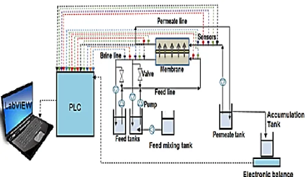
The pilot scale DCMD unit that was used in this work is shown in Fig. 1 with a counter current flow of the hot and cold streams. This pilot scale unit was comprised of 3 independent streams: the hot feed stream, recirculated brine and cold distillate collected from the overflow of the distillate tank inside a container which was situated on an electronic balance. The electronic balance was used to measure the mass flowrate of the distillate produced. The hot feed and cold distillate circuits include mainly a buffer tank, recirculation pump and temperature transmitters. The buffer tank was used to collect the brine discharged from the unit. The brine was then recirculated back to the feed line through the recirculation pump. The cold distillate was collected in a distillate tank from where it was also recirculated back to the cold side of the cross-flow DCMD configuration. The hot feed stream contained an electrical heater to set the feed temperature while the cold distillate stream contained a cooler to set the inlet cold stream to the required temperature. However, temperature transmitters were used to control the temperature of the inlet feed and cold stream to the hot and cold channels of the configuration, respectively. The individual parts were connected to each other via pipes. A plate-and-frame DCMD module was used in the test facility. The membrane used was made of polyethylene material which has high intrinsic hydrophobicity with low surface energy, good chemical stability, low thermal conductivity, and is commercially available [32]. The porosity, thickness and effective membrane area were 85%, 75 μm, and 0.05 m2
, respectively. The fully automated pilot scale unit with a programmable logic controller (PLC) control was connected to a computer with LabVIEW-based software tool for data acquisition, measurement analysis, data logging, instrument control, and report generation. All sensors in the experimental facility are connected to the PLC. These sensors were: the weighing balance sensor for continuous online monitoring of distillate production; sensors for monitoring the temperature, pressure, and flow rate at the inlets and outlets of the hot and cold channels; and sensors for continuous online monitoring of distillate and brine conductivities at the inlet and outlets of the hot and cold channels.
Synthetic NaCl solution was used as the feed of the pilot facility. This solution was prepared by dissolving analytical-grade NaCl salt purchased from Sigma Aldrich in deionized water. The feed and permeate were made to flow in a countercurrent mode and their temperatures were regulated using the temperature transmitters in the pilot facility. The permeate was discharged from the cold channel to the distillate tank, from where it is recirculated back to the cold channel. The permeate that overflowed from the outlet of the distillate tank was collected in the distillate collection (overflow) pan, which was placed on a weighing balance. The specifications of the experimental facility equipment are as follows:
6
Fig. 1. Schematic of the flows and devices in the pilot-scale DCMD unit showing counter current flow of the hot and cold streams. The specifications and dimensions of the components of the
experimental facility are given as follows:
− Circulation tanks: The feed or brine circulation tank was cylindrical and it was made from polypropylene. It had a diameter of 200 mm and height of 600 mm with connections to the feed stream, return stream, overflow and drain. It was connected to a pump with maximum flow rate of 10 L/min. It had an electrical flow control system that could regulate flow properties to the following limits: brine flow rate at 20-250 L/h and brine conductivity at 0.5-500 mS/cm. The permeate or distillate circulation tank had the same dimensions as the brine circulation tank and it was connected to the permeate stream, return stream, overflow and drain. It was also made from polypropylene. It was connected to a pump with maximum flow rate of 10 L/min. It had the same electrical flow control system as that of the brine circulation tank.
− Brine heater: The brine heater was spiral in shape. It was located inside the feed or brine circulation tank. It was an electrical heater with a power of 3 kW (220V, spiral diameter of 125 mm, and height of 410 mm). It was also connected to a temperature transmitter and level switch.
− Distillate cooler: It was a polypropylene tank with dimensions ø200 x 700 mm that contained a spiral heat exchanger with a length of 200 mm and diameter of 100 mm.
− Permeate or distillate collection pan: It ws a polypropylene tank with dimensions of ø140 x 600 mm. It was connected to a pump with maximum flow rate of 10 L/min.
7
− Membrane module: It was made from polypropylene and had external dimensions of 600 x 200 x 50 mm and internal dimensions of 500 x 100 x 4 mm. The polypropylene channels contained diamond spacers with thickness of 2 mm.
− e-Cabinet: The e-Cabinet contained the PLC connected to a computer with LabVIEW. − The control loops are:
a. Brine flow control: The flow of the brine was controlled by a frequency controlled pump which received an electrical signal from a flow controller. b. Distillate flow control: The flow of the distillate was controlled by a
frequency controlled pump which received an electrical signal from a flow controller.
c. Top temperature control: The top temperature (of feed or recirculated brine) entering the module was controlled by an electrical heater which received an electrical signal from a temperature controller.
d. Low temperature control: The low temperature (of recirculated permeate) entering the module was controlled by a frequency-controlled cooling water pump which received an electrical signal from a temperature controller. e. Heater control: It was used to regulate the heater. It contained a level switch
which would automatically switch off the heater when the water level was too low in the tank. Also, if the temperature measured in the tank was above 95oC, the heater would be switched off automatically.
2.2 Experimental design and statistical analysis
The sensitivity of three performance indicators (distillate production rate, recovery ratio, and performance ratio) to changes in operating conditions was studied. Firstly, a design of experiment (DoE) was carried out by using 5 control factors (feed flowrate, feed inlet temperature, feed concentration, distillate flowrate, and distillate temperature). For each factor, four levels were used. These levels are denoted by the numbers 1, 2, 3 and 4 in the columns of Table 1 while the control factors are listed in the rows.
Table 1. The test factors and levels.
Factor (k) Unit
Level (t)
1 2 3 4
Hot feed flowrate L/min 0.67 1.00 1.30 1.60
Hot feed inlet temperature
o
C 40 50 70 90
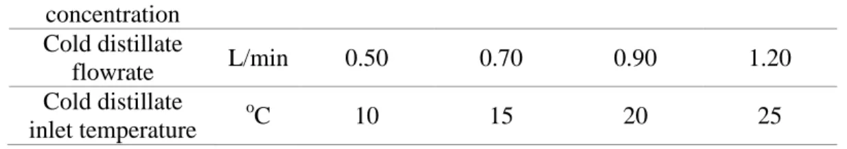
8 concentration Cold distillate flowrate L/min 0.50 0.70 0.90 1.20 Cold distillate inlet temperature o C 10 15 20 25
These levels were selected because they were considered as the operating ranges for normal or feasible DCMD operations using the experimental setup. Beyond these ranges, the setup used for this study would not function appropriately. Since there were 5 controls factors and 4 levels of each factor were tested, 45 number of experiments would normally be required if each factor was varied while other factors were kept constant (at each level) – in accordance with factorial DoE. However, this approach is not efficient. The sensitivity analysis has, therefore, been carried out by using the orthogonal array design.
The notation 𝐿𝑛 (𝑡𝑘) was used to express the orthogonal array experimental design, where 𝐿 refers to the Latin square arrangement of factors. 𝑛 denotes the number of experimental trials, k is the number of factors investigated and 𝑡 is the number of levels of each factor investigated. The orthogonal array used in the experiment design was 𝐿14, which means that only 14 experiment trials were required instead of the 45 (complete bicubic form) or 1,024 trials that would normally be required for the full 45 factorial design. All experimental trials of the orthogonal array 𝐿14(45) for the partial k-cubic interpolation used in this study are summarized in Table 2. Each row of Table 2 represents an experimental trial. In each trial, each factor was specified at one of the four levels.
Table 2. Experimental layout using an L14 (45) orthogonal array.
Experimental run Level Hot feed flowrate (L/min)
Hot feed inlet temperature (oC) Hot feed concentration (ppm) Cold distillate flowrate (L/min) Cold distillate inlet temperature (oC) 1 0.67 40 10,000 0.50 10 2 0.67 50 30,000 0.70 15 3 0.67 70 40,000 0.90 20 4 0.67 90 50,000 1.20 25 5 1.00 40 30,000 0.90 25 6 1.00 50 10,000 1.20 20 7 1.00 70 50,000 0.50 15
9 8 1.00 90 40,000 0.70 10 9 1.30 40 40,000 1.20 15 10 1.30 70 10,000 0.70 25 11 1.30 90 30,000 0.50 20 12 1.60 50 40,000 0.50 25 13 1.60 70 30,000 1.20 10 14 1.60 90 10,000 0.90 15
2.3 Pearson’s product momentum
The correlations between each performance indicators and the control factors were studied by using the Pearson’s product momentum correlations coefficients. From these coefficients, the most significant factors influencing each performance indicator were selected and analyzed. The influence of the selected factors on the DCMD performance indicators was further studied in 3D (i.e. by taking two factors and one performance indicator at a time) through response surface analysis. Pearson’s product momentum correlation coefficient rp was used to obtain the strength
and direction of correlations between each control factor and a performance indicator - X and Y, respectively, as shown in Eq. (2).
2 2 ) ( ) ( ) )( ( avg avg avg avg p Y Y X X Y Y X X r − − Σ − − Σ = (2)
where Xavg. and Yavg. are the mean values of X and Y, respectively. Generally, the value of rp
oscillates between -1 and +1, as rp = -1 or rp = +1 represents a perfect correlation, and rp = 0
shows no correlation. Positive rp shows a direct proportionality, while the negative rp shows an
inverse or opposite proportionality. The statistical analysis for the estimation of the Pearson’s product momentum correlations coefficients was carried out using Microsoft Excel built-in functions.
2.4 Response surface analysis
The most significant operating factors were obtained from correlation analysis. However, the results obtained from the correlation analysis were further analyzed by using response surface charts to investigate the influence of the control factors on the DCMD performance indicators. . Response surface analysis is a combination of mathematical and statistical techniques, which can be well applied when a response or a set of responses of interest are influenced by several variables. The objective is to optimize simultaneously the levels of these variables to attain an optimal system performance. Therefore, the response surface charts provided the 3D illustration of the response of each performance indicator to changes in two significant control factors. The
10
colors in the regions/zones of the response surface charts show the strata of the magnitudes of the dependent variables.
The modeled DCMD performance indicators, which were obtained statistically from the actual experimental performance indicators, were the responses of the orthogonal array design. The actual experimental cold distillate production rate, performance ratio, and recovery ratio are denoted as Y1, Y2, and Y3, respectively. Codes were also used to represent the control factors (input variables) and the responses of the performance indicators (output variables). The control factors were represented by Xk while the responses were defined by Ŷq (q is the notation of
responses). Ŷq include Ŷ1, Ŷ2, and Ŷ3, which are the computed responses of the cold distillate production rate, performance ratio, and recovery ratio, respectively.
The responses of Y1 to the levels of X1 were obtained by computing the L averages of Y1 (i.e. Ŷ1𝑋1 = 1, Ŷ1𝑋1 = 2, …, Ŷ1𝑋1 = 𝐿1). Ŷ1𝑋1 = 1 is the average of the values of Y1 obtained at the first level of X1, i.e. when X1 was 0.67 L/min. Ŷ1𝑋1 = 2 to Ŷ1𝑋1 = 𝐿1 are the averages of the values of Y1 obtained at the second to the last level of X1. Similarly, the responses of Y1 to the levels of other control factors were computed (i.e. Ŷ1𝑋2 = 1 to Ŷ1𝑋2 = 𝐿2; Ŷ1𝑋3 = 1 to Ŷ1𝑋3 = 𝐿3; Ŷ1𝑋4 = 1 to Ŷ1𝑋4 = 𝐿4; Ŷ1𝑋5 = 1 to Ŷ1𝑋5 = 𝐿5). Then, the responses of Y2 and Y3 to each level of all control factors were calculated. In general, (3) was used to calculate Ŷq at different levels of all control factors 𝑋𝑘. Ŷq𝑋𝑘 = 1= ∑𝐿2𝑗=1∑𝐿3𝑙=1∑𝐿4𝑚=1∑𝐿5𝑛=1𝑌1,𝑗,𝑙,𝑚,𝑛 L2𝐿3𝐿4𝐿5 … Ŷq𝑋𝑘 = 𝐿𝑘 = ∑𝐿2𝑗=1∑𝐿3𝑙=1∑𝐿4𝑚=1∑𝑛=1𝐿5 𝑌Li,𝑗,𝑙,𝑚,𝑛 L2𝐿3𝐿4𝐿5 (3)
The notations for all responses and factors are shown in Table 3. Since four levels of each factor were used, these levels were indicated by 𝐿1, 𝐿2, …, 𝐿𝑘, respectively.
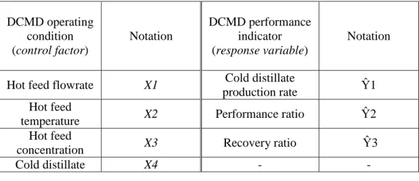
Table 3. Notations for all factors and responses.
DCMD operating condition (control factor) Notation DCMD performance indicator (response variable) Notation
Hot feed flowrate X1 Cold distillate
production rate Ŷ1 Hot feed
temperature X2 Performance ratio Ŷ2
Hot feed
concentration X3 Recovery ratio Ŷ3
11 flowrate
Cold distillate
inlet temperature X5 - -
The main effects of the factors on the responses of each performance indicator (𝑀𝑋𝐾Ŷq)were then obtained. For example, the main effects of the factors on Ŷ1 were computed from (4a)-(4e). 𝑀𝑋1Ŷ1 = ∑ (𝐿1 𝑖=1 Ŷ1𝑋1=𝑖− Y�1)2 (4a) 𝑀𝑋2Ŷ1 = ∑ (𝐿2 𝑗=1 Ŷ1𝑋2=𝑗− Y�1)2 (4b) 𝑀𝑋3Ŷ1 = ∑ (𝐿3 𝑙=1 Ŷ1𝑋3=𝑙− Y�1)2 (4c) 𝑀𝑋4Ŷ1 = ∑𝐿4 ( 𝑚=1 Ŷ1𝑋4=𝑚 − Y�1)2 (4d) 𝑀𝑋5Ŷ1 = ∑𝐿5 ( 𝑛=1 Ŷ1𝑋5=𝑛− Y�1)2 (4e)
Y�1 is the overall average of Y1 obtained from all experimental trials or samples. The main effects of the factors on the responses of Y2 and Y3 were computed in the same manner and adapted from (4a)–(4e). For each response, the overall average Y�𝑞 was computed from (5).
Y�𝑞 =∑𝐿1𝑖=1∑𝐿2𝑗=1∑𝐿3𝑙=1∑𝐿4𝑚=1∑𝐿5𝑛=1𝑌𝑖,𝑗,𝑙,𝑚,𝑛
𝑁 (5)
N is the sample size of this adjustable factorial design containing k factors 𝑋1, …, 𝑋𝑘 with 𝐿1, …, 𝐿𝑘 levels, respectively. N was estimated from Eq. (6).
𝑁 = ∏𝑘𝑖=1𝐿𝑖 (6)
From 𝑀𝑋𝑘Ŷq, the two factors that exhibited the greatest influence on each response variable were selected. 𝑀𝑋𝑘Ŷq ensured that the influence of all control factors on each performance indicator could be observed quantitatively and in a statistical manner. The larger the value of 𝑀𝑋𝑘Ŷq, the greater would be the influence of 𝑋𝑘 on Ŷq.
The interaction effect between the two factors that provided the greatest influence on each performance indicator was then calculated from (7) and (8), in order to observe the inter-dependence between these selected factors.
12 Ŷ𝑋1=1,𝑋2=1= ∑𝐿3𝑙=1∑𝐿4𝑚=1∑𝐿5𝑛=1𝑌1,2,𝑙,𝑚,𝑛 𝐿3𝐿4𝐿5 … Ŷ𝑋1=𝐿1,𝑋2=𝐿2 = ∑𝐿3𝑙=1∑𝐿4𝑚=1∑𝐿5𝑛=1𝑌L1,L2,𝑙,𝑚,𝑛 𝐿3𝐿4𝐿5 (7) 𝑀𝑋1,𝑋2 = ∑ ∑ ( 𝐿2 𝑗=1 𝐿1 𝑖=1 Ŷ𝑋1=𝑖,𝑋2=𝑗 − Ŷ)2− 𝑀𝑋1− 𝑀𝑋2 (8) 3. Results and discussion
3.1 Experimental design with orthogonal arrays
The values of Ŷq obtained at different levels of 𝑋𝑘 are shown in Fig. 2. Fig. 2(a) shows the response of cold distillate production rate to different levels of the control factors. It was observed that the distillate production rate was mostly influenced by the hot feed and the cold distillate inlet temperature. The influence of feed temperatures and the vapor pressure dependence of flux on temperature (i.e., Antoine's equation) is well understood and presented in many prior MD papers. The increase in hot feed temperature increased the kinetics and thermodynamic property of the flow of the feed, which could be defined by the relative importance of momentum and viscous forces, and thereby improved the hydrodynamics of the feed adjacent to the membrane [33]. This reduced the thickness of the thermal and solute boundary layers near the membrane, increased the heat and mass transfer coefficients, and ultimately resulted in an increase in cold distillate production rate [34]. Fig. 2(b) shows the effect of the changing levels of the factors on the performance ratio. The performance ratio was mostly influenced by the cold distillate temperature. The possible explanation is that less cold distillate temperature improved the driving force of heat transfer and enhanced the pressure gradient that propelled the transport of vapor to the distillate side of the membrane. It can also be observed from Fig. 2(b) that the performance ratio was strongly influenced by the highest level of feed temperature. Since high rate of distillate production was also observed at this level, this can be explained by the increase in the heat input which resulted in high rate of thermal energy utilization at this level.
13 (a) (b) 0 0,05 0,1 0,15 0,2 0,25 0,3 X1 X2 X3 X4 X5 Ŷ 1 ( g/ s) 1 2 3 4 0 0,005 0,01 0,015 0,02 0,025 0,03 0,035 0,04 0,045 0,05 X1 X2 X3 X4 X5 Ŷ2 1 2 3 4
14 (c)
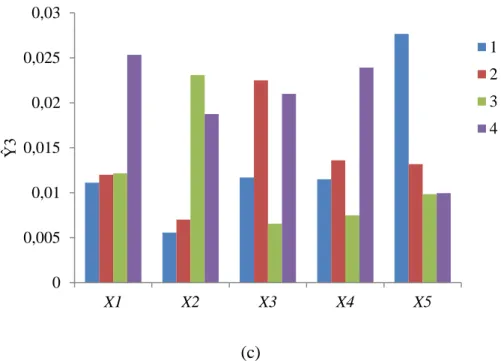
Fig. 2. Predicted responses of (a) distillate production rate; (b) performance ratio; (c) recovery ratio to different levels of the control factors. The levels are indicated as 1, 2, 3 and 4. The four levels of the five factors are: X1 = 0.67, 1.00, 1.30, and 1.60 L/min; X2 = 40, 50, 70, and 90oC; X3 = 10,000, 30,000, 40,000, and 50,000 ppm; X4 = 0.50, 0.70, 0.90, and 1.20; X5 = 10, 15, 20, and 25oC. Ŷ1, Ŷ2, and Ŷ3 are the averages (responses) of the values of cold distillate production rate, performance ratio, and recovery ratio, respectively, at different levels of the factors. For example, Ŷ𝑋1=1 is the average of the values of cold distillate production rate obtained at the first
level of X1, i.e. when X1 was 0.67 L/min.
The increase in the cold distillate production means that high thermal energy was required to vaporize pure water from the feed; hence, higher performance ratio was ensured by the system at this condition [31,34]. The increase in the hot feed temperature improved the ratio of energy demand by the system to that supplied to the system. Fig. 2(c) shows a similar trend with Fig. 2(b). The recovery ratio was mostly influenced by the increase in the hot feed temperature and the decrease in the cold distillate temperature. This resulted in an increase in the rate of cold distillate production for every feed flowrate; hence an increase in recovery rate was ensured. These effects can also be explained by the results obtained from the computations of the main effects between the responses and factors (𝑀𝑋𝑘), as shown in Table 4. For each responseŶq, the main effects are indicated by 𝑀Ŷq𝑋𝑘 in the table. It was observed that the main effects of feed and distillate temperatures on all responses were the greatest. For distillate production rate and performance ratio, the effect of changes in the levels of feed temperature was higher than that of distillate temperature (and this effect was more pronounced on distillate production rate). The recovery ratio was more influenced by the changes in cold distillate temperatures because, as
0 0,005 0,01 0,015 0,02 0,025 0,03 X1 X2 X3 X4 X5 Ŷ3 1 2 3 4
15
expected, a higher recovery ratio would be achieved at higher pressure gradients between the adjacent sides of the membrane, even when the feed temperature is kept constant.
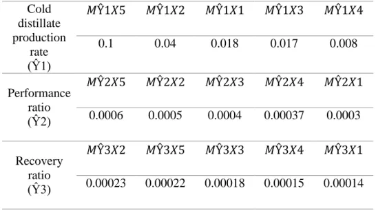
Table 4. The main effects of control factors on the responses. The main effects are indicated by 𝑀Ŷq𝑋𝑘 for each response Ŷq. Ŷq include Ŷ1, Ŷ2, and Ŷ3. 𝑀Ŷq𝑋𝑘 is the main effect of a control
factor 𝑋𝑘 on a performance indicator Ŷq. Cold distillate production rate (Ŷ1) 𝑀Ŷ1𝑋5 𝑀Ŷ1𝑋2 𝑀Ŷ1𝑋1 𝑀Ŷ1𝑋3 𝑀Ŷ1𝑋4 0.1 0.04 0.018 0.017 0.008 Performance ratio (Ŷ2) 𝑀Ŷ2𝑋5 𝑀Ŷ2𝑋2 𝑀Ŷ2𝑋3 𝑀Ŷ2𝑋4 𝑀Ŷ2𝑋1 0.0006 0.0005 0.0004 0.00037 0.0003 Recovery ratio (Ŷ3) 𝑀Ŷ3𝑋2 𝑀Ŷ3𝑋5 𝑀Ŷ3𝑋3 𝑀Ŷ3𝑋4 𝑀Ŷ3𝑋1 0.00023 0.00022 0.00018 0.00015 0.00014
3.2 Correlation analysis - Pearson’s product momentum
Pearson product-moment correlation coefficients showed the statistical dependence between the control factors (independent variables) and performance indicators (dependent variables). Fig. 3 below shows the coefficients of correlation between each DCMD performance indicator and the factors. It can be seen from Fig. 3 that the cold distillate production rate was mostly correlated with the hot feed inlet temperature (as also obtained from the orthogonal array design). Therefore, the hot feed inlet temperature played the most significant role in determining the rate of cold distillate production and these two variables were positively correlated, with a correlation coefficient of rp = +0.61. This correlation analysis confirmed the results obtained from the
orthogonal array design modeling – all performance indicators were mostly influenced by the hot feed and cold distillation temperatures, as again the flowrates and concentration of these streams. The performance and recovery ratios were both noticeably influenced by cold distillate and hot feed inlet temperature, with rp = -0.43 and rp = +0.44, respectively, for both factors. As it can be
seen from Fig. 3, the cold distillate temperature was inversely correlated to these ratios. The transfer of heat required for the condensation of vapor produced from the DCMD process and the mass transfer required to enhance the recovery ratio were favored by decreasing levels of cold distillate temperature. Conversely, the performance and recovery ratios were directly influenced
16
by the hot feed inlet temperature. Heat and mass transfer required for fresh water production and energy efficiency were favored by higher levels of feed inlet temperature [20]. The required heat input to the DCMD process was considerably dependent on feed properties such that the supply and utilization of thermal energy required for the operational efficiency of the DCMD process was significantly favored by feed temperature.
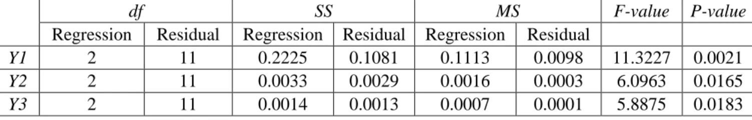
At confidence interval of 95%, the statistical significance of the correlation coefficients were determined by conducting an analysis of variance (ANOVA) between the DCMD performance indicators and responses obtained from the two most significant factors – X2 and X5. The results of this analysis are shown in Table 5. Since α = 0.05, the Pearson correlation coefficients would be only statistically significant at P-values ≤ 0.05. All the P-values obtained were less than 0.05, which signified that the dependence of the performance indicators on X2 and X5 was statistically significant. The statistical significance of the variables was also evaluated by using the F-value (a measurement of variance about the mean based on the group variance ratio). For all responses, the calculated F-values were greater than the critical F-values at a significant level of 5%, which further confirmed that the dependence between the responses and X2 and X5 was statistically significant. -0,6 -0,4 -0,2 0 0,2 0,4 0,6 0,8 Y1 Y2 Y3 C o rr el at io n co ef fi ci en t X1 X2 X3 X4 X5
17
Fig. 3. Pearson coefficients of correlation between DCMD performance indicators and control factors. The control factors are represented by X1 to X5 while the performance indicators are represented by Y1 to Y3. Positive values of correlation coefficient indicate direct dependence
whereas negative values indicate inverse dependence.
Table 5. ANOVA table for the statistical significance of correlation coefficients.
df SS MS F-value P-value
Regression Residual Regression Residual Regression Residual
Y1 2 11 0.2225 0.1081 0.1113 0.0098 11.3227 0.0021
Y2 2 11 0.0033 0.0029 0.0016 0.0003 6.0963 0.0165
Y3 2 11 0.0014 0.0013 0.0007 0.0001 5.8875 0.0183
*df = degrees of freedom; SS = sum of squares; MS = mean squared.
3.3 Response surfaces
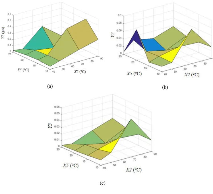
The effects of the factors on the orthogonal design responses were investigated through response surface charts, by examining the influence of two most significant factors on each response. The response surface charts provided the three-dimensional illustration of the variation of each response to changes in the most significant independent variables. The colors in the regions/zones of the response surface charts showed the differences between the magnitudes of the dependent variables. The response surface charts that show the variation of the performance indicators to changes in X2 and X5 are presented in Fig. 4. As it can be observed from Fig. 4(a), the maximum distillate rate was obtained when the hot feed temperature was 90oC. At the highest feed flow rate of 1.60 L/min, low distillate production rate was observed when the feed temperature was kept at the lowest value of 40oC (Table 6). Therefore, an increase in X1 without a corresponding increase in X2 did not result in improved productivity [35,36]. In addition, X2 influenced the heat input utilization more profoundly than X1. The heat input to the system is shown in Table 6. When both X1 and X2 were increased to their maximum values, a maximum heat input utilization of 37,500 J/s was achieved. Meanwhile, the relationship between the rate of cold distillate production rate and hot feed temperature was not linear and did not also follow the regular non-linear shapes. The relationship was characterized by a mountainous pattern but with a surging vortex towards the maximum points at the edges of Y1, as shown in Fig. 4(a).
The rate of cold distillate production was also significantly influenced by cold distillate temperature; as the response of the cold distillate production rate to changes in the cold distillate temperature was provided by an undulating or wave-like pattern that indicated repeating descent and ascent of cold distillate production rate as the cold distillate temperature increased.
18
Expectedly, for most real distillation processes, an increase in hot feed temperature would lead to an increase in distillate production because more distillate would be produced when a higher quantity of pure water is evaporated from a feed source with significant heat content [1,26]. Meanwhile, a low cold distillate temperature would not necessarily enhance the removal of enough heat of condensation from the vapor, as this extraction depends on the driving force and efficiency of heat transfer, membrane characteristics, flow dynamics, polarization effects and number of stages in the system [33,35,37,38]. The distillate production rates obtained at the minimum and maximum values of X5 were lower than the maximum value of Y1 obtained from this study. The optimum cold distillate production rate was obtained at the maximum value of X2. The electrical conductivity of the cold distillate produced at optimum value of X2 was 149.8 μS/cm, which was equivalent to salinity of 96 ppm.
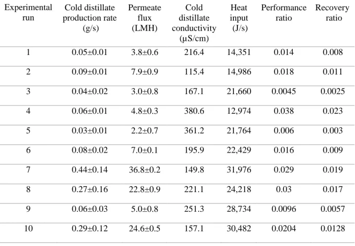
Table 6. Experimental results of cold distillate conductivity (µS/cm), heat input (J/s), performance ratio, and recovery ratio.
Experimental run
Levels of test factors Cold distillate production rate (g/s) Permeate flux (LMH) Cold distillate conductivity (µS/cm) Heat input (J/s) Performance ratio Recovery ratio 1 0.05±0.01 3.8±0.6 216.4 14,351 0.014 0.008 2 0.09±0.01 7.9±0.9 115.4 14,986 0.018 0.011 3 0.04±0.02 3.0±0.8 167.1 21,660 0.0045 0.0025 4 0.06±0.01 4.8±0.3 380.6 12,974 0.038 0.023 5 0.03±0.01 2.2±0.7 361.2 21,764 0.006 0.003 6 0.08±0.02 7.0±0.1 195.9 22,429 0.016 0.009 7 0.44±0.14 36.8±0.2 149.8 31,976 0.029 0.019 8 0.27±0.16 22.8±0.9 221.1 24,218 0.03 0.017 9 0.06±0.03 5.0±0.8 251.3 28,734 0.0096 0.0057 10 0.29±0.12 24.6±0.5 157.1 30,482 0.0204 0.0128
19
11 0.22±0.11 18.7±0.6 448.3 30,634 0.028 0.018
12 0.01±0.0 1.1±0.2 340.4 18,265 0.003 0.001
13 0.19±0.13 16.0±0.1 490.5 38,019 0.09 0.058
14 0.51±0.18 43.2±0.4 126.6 38,003 0.027 0.017
* Performance and recovery ratios were reported for 1 membrane element used in this study. However, the total number of membrane elements that can be used during operation is up to 6 membranes which can hence increase both performance and recovery ratios.
Therefore, the effect of the hot feed temperature on distillate production rate was more pronounced than that of the distillate inlet temperature. At the maximum value of X2, the value of X5 that was required to achieve the optimum distillate production rate of 0.51 g/s or flux of 43.2±0.4 LMH was 15oC (and not the lowest value of 10oC). In order not to jeopardize Y1 during the optimization of X5, a tradeoff or balance was required [20]. It would be technically and economically beneficial to operate at the highest value of X2 and at X5 = 10oC in order not to adversely affect the rate of cold distillate production since the electrical conductivity of the cold distillate produced at these maximum input values was still within the acceptable limit for fresh water. The shapes of the response surfaces charts for Y2 and Y3 are similar (Figs 4(b) and 4(c)).
20
Fig. 4. Response surfaces showing the effects of hot feed temperature (X2) and cold distillate temperature (X5) on (a) cold distillate production rate (Y1), (b) performance ratio (Y2), and (c)
recovery ratio (Y3).
The performance and recovery ratios were reported for 1 membrane element used in this study, however, the total number of membrane elements that can be used during operation is up to 6 membranes. The ratios were interrelated because a high performance ratio was required to ensure high recovery of product water from the feed, which invariably affected the thermal energy utilization by the process [39]. Therefore, as efforts were geared towards the optimization of the
(a) (b)
21
recovery of the product water from the hot saline feed water, the optimization of the performance ratio of the DCMD process was equally important for energy and economic considerations [40,41]. By keeping the X2 low, the performance ratio can be optimized and hence, the heat input requirement for the process can be minimized. However, operating the DCMD process at low X2 would affect the process in terms of reduction in cold distillate production rate. Therefore, there is a need to determine the optimum values of X2 that would lead to savings in heat input and at the same time, augment cold distillate production. These optimum values are the values that provide the maximum performance ratio. The maximum performance ratio of 0.09 was obtained when X2 was 70oC. The highest performance ratio was not achieved while operating at the maximum temperature of 90oC because a higher heat input was required by the system at this maximum value. Despite the associated gain in cold distillate production at the maximum value of X2, the energy requirement of the system was affected.
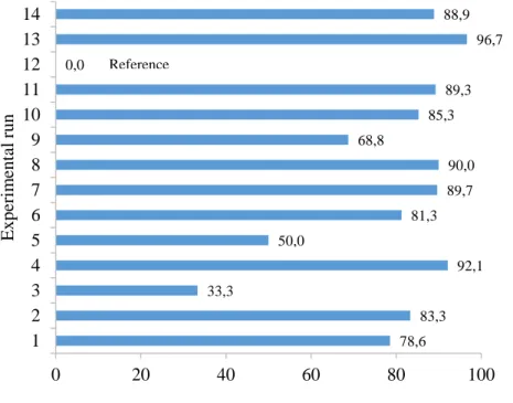
Fig. 5. % Increase in performance ratio for all experimental runs, relative to the lowest value (reference) obtained in experimental trial #12.
Consequently, Fig. 4(b) provides that the optimal performance ratio would only be achievable at 70oC, rather than at 90oC. This is further illustrated in Fig. 5, where the incremental percentage in performance ratio is shown quantitatively. The lowest performance ratio was obtained from experimental run #12. The incremental percentage was the extent to which the performance ratio obtained for each run exceeds the lowest performance ratio. It can be observed that the highest incremental percentage of 96.7% was achieved in experimental run #13, when the feed
78,6 83,3 33,3 92,1 50,0 81,3 89,7 90,0 68,8 85,3 89,3 0,0 96,7 88,9 0 20 40 60 80 100 1 2 3 4 5 6 7 8 9 10 11 12 13 14
% Relative increase in performance ratio
E xpe ri m ent al r un Reference
22
temperature was 70oC. The performance ratio can be expressed as recovery ratio multiplied by the latent heat of vaporization of fresh water per unit heat input. Therefore, the surface charts for the performance and recovery ratios were similar because the heat input to the DCMD process at optimized values of X2 and X5 would affect both performance indicators analogously [42]. Therefore, both ratios are constant through the heat input to the DCMD process and the latent heat of condensation of water, which can be obtained as a constant at the optimized values of X2 and X5 [42].
4. Conclusions
In this work, an orthogonal (fractional factorial) experimental design was used to identify the operating factors that most significantly affect the distillate production rate, performance ratio and recovery ratio in a DCMD process. Results were obtained for these performance indicators from fourteen experiments by controlling these operating factors - hot feed properties (temperature, salinity, flow rate) and the cold distillate characteristics (temperature and flow rate). The orthogonal experimental design also permitted the determination of the optimal values of the five factors based on the fourteen experiments. The main and interaction effects obtained from this experimental design indicated that the most significant factors were the feed and distillate temperatures. This observation was also confirmed by using Pearson product-moment correlation and response surface analyses. The correlation and response surface analyses indicated that the hot feed and cold distillate temperatures were the dominant factors. These factors gave the highest correlation coefficients (for all performance indicators). The distillate production rate obtained from the experimental run where these optimal values (e.g. 1.60 L/min, 90oC, 10,000 ppm, 0.90 L/min and 15oC for feed flow rate, feed temperature, feed salinity, distillate flow rate and distillate temperature, respectively) were used surpassed the distillate production rates obtained from the other experimental runs. Meanwhile, for the response surface charts, the maximum performance ratio of 0.09 was obtained when the feed temperature was 70oC. The maximum performance ratio was not achieved while operating at the highest feed temperature of 90oC because a higher heat input was required by the system at this maximum temperature. The extra heat input required to raise the feed temperature from 70 to 90oC resulted in a decrease in the performance ratio despite the gain in distillation production rate that was associated with this rise in temperature. It is worth noting that the values of the five factors that gave the highest cold distillate production do not represent the global optimum.Although it has already been established in membrane distillation that temperature difference between hot feed and cold distillate is a significant determining factor for distillate productivity, the predominance of feed/coolant temperatures over other factors have never been established. Many studies have only concluded that operating factors hugely determine the extent to which the temperature gradient driving force affects distillate productivity. In this study, we have established through statistical analysis that feed/coolant temperatures affect distillate productivity - by a greater scale of statistical significance – more than the other considered operating factors. In addition, no
23
study has attempted before now to study the degree to which performance and recovery ratios are influenced by different operating conditions in DCMD. The statistical evaluation of the influence of each operating factor on performance and recovery ratios would be particularly useful for the optimization of the process economics and scale-up. To choose the right conditions, the understanding of the relative influence of each operating factor is required. In the future, the optimal values obtained from the fourteen runs would be used for testing a DCMD system for a long period of time to evaluate the commercial feasibility of implementing it in the Gulf region.
Acknowledgement
Authors would like to thank Masdar Institute of Science and Technology (Masdar Institute Fellowship Program (MIFP)) for its support towards the achievement of the objectives of this research.
References
[1] A. Giwa, H. Fath, S.W. Hasan, Humidification–dehumidification desalination process driven by photovoltaic thermal energy recovery (PV-HDH) for small-scale sustainable water and power production, Desalination. 377 (2016) 163–171.
doi:10.1016/j.desal.2015.09.018.
[2] A. Abusharkh, A. Giwa, S. Hasan, Wind and geothermal energy in desalination: A short review on progress and sustainable commercial processes, Ind. Eng. Manag. 4 (2015) 175. doi:10.4172/2169-0316.1000175.
[3] S. Jamaly, A. Giwa, S.W. Hasan, Recent improvements in oily wastewater treatment: Progress, challenges, and future opportunities, J. Environ. Sci. 37 (2015) 15–30. doi:10.1016/j.jes.2015.04.011.
[4] S. Daer, J. Kharraz, A. Giwa, S.W. Hasan, Recent applications of nanomaterials in water desalination: A critical review and future opportunities, Desalination. 367 (2015) 37–48. doi:10.1016/j.desal.2015.03.030.
[5] N. Akther, A. Sodiq, A. Giwa, S. Daer, H.A. Arafat, S.W. Hasan, Recent advancements in forward osmosis desalination: A review, Chem. Eng. J. 281 (2015) 502–522.
doi:10.1016/j.cej.2015.05.080.
[6] A. Giwa, S.W. Hasan, Theoretical investigation of the influence of operating conditions on the treatment performance of an electrically-induced membrane bioreactor, J. Water Process Eng. 6 (2015) 72–82. doi:10.1016/j.jwpe.2015.03.004.
[7] A. Giwa, I. Ahmed, S.W. Hasan, Enhanced sludge properties and distribution study of sludge components in electrically-enhanced membrane bioreactor., J. Environ. Manage. 159 (2015) 78–85. doi:10.1016/j.jenvman.2015.05.035.
24
[8] A. Giwa, S.W. Hasan, Numerical modeling of an electrically enhanced membrane
bioreactor (MBER) treating medium-strength wastewater, J. Environ. Manage. 164 (2015) 1–9. doi:10.1016/j.jenvman.2015.08.031.
[9] M. Zeyoudi, E. Altenaiji, L.Y. Ozer, I. Ahmed, A.F. Yousef, S.W. Hasan, Impact of continuous and intermittent supply of electric field on the function and microbial community of wastewater treatment electro-bioreactors, Electrochim. Acta. (2015). doi:10.1016/j.electacta.2015.04.095.
[10] D.M. Warsinger, J. Swaminathan, E. Guillen-Burrieza, H. a. Arafat, J.H. Lienhard V, Scaling and fouling in membrane distillation for desalination applications: A review, Desalination. 356 (2014) 294–313. doi:10.1016/j.desal.2014.06.031.
[11] A. Giwa, N. Akther, A. Al Housani, S. Haris, S.W. Hasan, Recent advances in
humidification dehumidification (HDH) desalination processes: Improved designs and productivity, Renew. Sustain. Energy Rev. 57 (2016) 929–944.
doi:10.1016/j.rser.2015.12.108.
[12] Y. Zhang, Y. Peng, S. Ji, Z. Li, P. Chen, Review of thermal efficiency and heat recycling in membrane distillation processes, Desalination. 367 (2015) 223–239.
doi:10.1016/j.desal.2015.04.013.
[13] E. Drioli, A. Ali, F. Macedonio, Membrane distillation: Recent developments and perspectives, Desalination. 356 (2015) 56–84.
doi:http://dx.doi.org/10.1016/j.desal.2014.10.028.
[14] G.W. Meindersma, C.M. Guijt, a. B. de Haan, Desalination and water recycling by air gap membrane distillation, Desalination. 187 (2006) 291–301.
doi:10.1016/j.desal.2005.04.088.
[15] M.A.E.-R. Abu-Zeid, Y. Zhang, H. Dong, L. Zhang, H.-L. Chen, L. Hou, A
comprehensive review of vacuum membrane distillation technique, Desalination. 356 (2015) 1–14. doi:10.1016/j.desal.2014.10.033.
[16] M. Khayet, Solar desalination by membrane distillation: Dispersion in energy
consumption analysis and water production costs (a review), Desalination. 308 (2013) 89– 101. doi:10.1016/j.desal.2012.07.010.
[17] M.R. Qtaishat, F. Banat, Desalination by solar powered membrane distillation systems, Desalination. 308 (2013) 186–197. doi:10.1016/j.desal.2012.01.021.
[18] A. Alkhudhiri, N. Darwish, N. Hilal, Membrane distillation: A comprehensive review, Desalination. 287 (2012) 2–18. doi:10.1016/j.desal.2011.08.027.
[19] L.M. Camacho, L. Dumée, J. Zhang, J. De Li, M. Duke, J. Gomez, et al., Advances in membrane distillation for water desalination and purification applications, Water (Switzerland). 5 (2013) 94–196. doi:10.3390/w5010094.
25
[20] M. Khayet, C. Cojocaru, C. Garcia-Payo, Application of response surface methodology and experimental design in direct contact membrane distillation, Ind. Eng. Chem. Res. 46 (2007) 5673–5685 ST–Application of response surface me. doi:10.1021/ie070446p. [21] A.M. Alklaibi, N. Lior, Heat and mass transfer resistance analysis of membrane
distillation, J. Memb. Sci. 282 (2006) 362–369. doi:10.1016/j.memsci.2006.05.040. [22] A.M. Alklaibi, N. Lior, Comparative study of direct-contact and air-gap membrane
distillation processes, Ind. Eng. Chem. Res. 46 (2007) 584–590. doi:10.1021/ie051094u. [23] A.M. Alklaibi, N. Lior, Transport analysis of air-gap membrane distillation, J. Memb.
Sci. 255 (2005) 239–253. doi:10.1016/j.memsci.2005.01.038.
[24] O.K. Buros, The ABCs of Desalting, 2nd Ed., International Desalination Association, 2000.
[25] G. Burgess, K. Lovegrove, Solar thermal powered desalination: membrane versus
distillation technologies, in: 43rd Conf. Aust. New Zeal. Sol. Energy Soc., Dunedin, New Zealand, 2005.
[26] H.T. El-Dessouky, H.M. Ettouney, Fundamentals of Salt Water Desalination, 2002. doi:10.1016/B978-044450810-2/50008-7.
[27] A.M. El-Nashar, The economic feasibility of small solar MED seawater desalination plants for remote arid areas, Desalination. 134 (2001) 173–186. doi:10.1016/S0011-9164(01)00124-2.
[28] P. Sharan, S. Bandyopadhyay, Energy optimization in parallel/cross feed multiple-effect evaporator based desalination system, Energy. 111 (2016) 756–767.
doi:10.1016/j.energy.2016.05.107.
[29] S. Chung, C.D. Seo, H. Lee, J.-H. Choi, J. Chung, Design strategy for networking
membrane module and heat exchanger for direct contact membrane distillation process in seawater desalination, Desalination. 349 (2014) 126–135.
doi:10.1016/j.desal.2014.07.001.
[30] H. Chang, C.-L. Chang, C.-Y. Hung, T.-W. Cheng, C.-D. Ho, Optimization study of small-scale solar membrane distillation desalination systems (s-SMDDS), Int. J. Environ. Res. Public Health. 11 (2014) 12064–12087. doi:10.3390/ijerph111112064.
[31] S. Lin, N.Y. Yip, M. Elimelech, Direct contact membrane distillation with heat recovery: Thermodynamic insights from module scale modeling, J. Memb. Sci. 453 (2014) 498– 515. doi:10.1016/j.memsci.2013.11.016.
[32] J. Zuo, S. Bonyadi, T.-S. Chung, Exploring the potential of commercial polyethylene membranes for desalination by membrane distillation, J. Memb. Sci. 497 (2016) 239–247. doi:10.1016/j.memsci.2015.09.038.
26
[33] B.B. Ashoor, S. Mansour, A. Giwa, V. Dufour, S.W. Hasan, Principles and applications of direct contact membrane distillation (DCMD): A comprehensive review, Desalination. 398 (2016) 222–246. doi:10.1016/j.desal.2016.07.043.
[34] G. Chen, Y. Lu, W.B. Krantz, R. Wang, A.G. Fane, Optimization of operating conditions for a continuous membrane distillation crystallization process with zero salty water discharge, J. Memb. Sci. 450 (2014) 1–11. doi:10.1016/j.memsci.2013.08.034. [35] H.C. Duong, P. Cooper, B. Nelemans, T.Y. Cath, L.D. Nghiem, Optimising thermal
efficiency of direct contact membrane distillation by brine recycling for small-scale seawater desalination, Desalination. 374 (2015) 1–9. doi:10.1016/j.desal.2015.07.009. [36] J. Minier-Matar, A. Hussain, A. Janson, F. Benyahia, S. Adham, Field evaluation of
membrane distillation technologies for desalination of highly saline brines, Desalination. 351 (2014) 101–108. doi:10.1016/j.desal.2014.07.027.
[37] C.-D. Ho, C.-H. Huang, F.-C. Tsai, W.-T. Chen, Performance improvement on distillate flux of countercurrent-flow direct contact membrane distillation systems, Desalination. 338 (2014) 26–32. doi:10.1016/j.desal.2014.01.023.
[38] G. Guan, X. Yang, R. Wang, A.G. Fane, Evaluation of heat utilization in membrane distillation desalination system integrated with heat recovery, Desalination. 366 (2015) 80–93. doi:10.1016/j.desal.2015.01.013.
[39] T.Y. Cath, V.D. Adams, A.E. Childress, Experimental study of desalination using direct contact membrane distillation: A new approach to flux enhancement, J. Memb. Sci. 228 (2004) 5–16. doi:10.1016/j.memsci.2003.09.006.
[40] G. Zuo, R. Wang, R. Field, A.G. Fane, Energy efficiency evaluation and economic analyses of direct contact membrane distillation system using Aspen Plus, Desalination. 283 (2011) 237–244. doi:10.1016/j.desal.2011.04.048.
[41] V.A. Bui, L.T.T. Vu, M.H. Nguyen, Simulation and optimisation of direct contact membrane distillation for energy efficiency, Desalination. 259 (2010) 29–37. doi:10.1016/j.desal.2010.04.041.
[42] K. Mistry, J. Lienhard, An economics-based second law efficiency, Entropy. 15 (2013) 2736–2765. doi:10.3390/e15072736.