Efficient Dust Detection based on Spectral and Thermal Observations of
1
MODIS Imagery
2
Hazhir Bahramia, Saied Homayounib, Reza Shah-Hosseinia,*, Arash ZandKarimic, 3
Abdolreza Safaria 4
a University of Tehran, School of Surveying and Geospatial Engineering, Department of Photogrammetry and 5
Remote Sensing, Tehran, Iran
6
b Centre Eau Terre Environnement, Institut National de la Recherche Scientifique, Québec, Canada 7
c Department of Remote Sensing and GIS, Tabriz University, Tabriz, Iran 8
Abstract. The dust storm is one of the severe natural disasters that has been recently threatening the Middle East
9
region due to climate changes and human activities. This phenomenon has become a national crisis in some countries
10
in this region over the previous years, especially in spring and summer. This research aims to detect and monitor the
11
areas covered by the seasonal and occasional dust storm from MODIS (Moderate Resolution Imaging
12
Spectroradiometer) satellite imagery. MODIS imagery possesses impressive spectral and temporal characteristics that
13
are essential for such an environmental application of Earth observations. An efficient algorithm, based on the spectral
14
and statistical analysis of both thermal and reflectance bands of MODIS data, was developed through a decision tree
15
method. To this end, an index was proposed to detect the dusts over the land using the brightness temperature of
16
thermal bands. The results of the proposed algorithm were assessed utilizing ground-based observation of synoptic
17
stations. The proposed method showed high reliability and performance, as well as the automatic capability of dust
18
detection in land and sea areas of the image simultaneously. The evaluation of results showed that the proposed
19
algorithm could detect thin and thick dust storms with an overall accuracy of about 80%. Moreover, the dust
20
monitoring results visually agreed well with the Ozone Monitoring Instrument Aerosol Index (OMI-AI) dust products.
21 22
Keywords: Dust detection and monitoring, Brightness Temperature, MODIS Satellite Images, Middle East,
OMI-23
AI.
24 25
* Reza Shah-Hosseini, E-mail: [email protected] 26
1 Introduction 27
Dust storms are one of the most hazardous environmental phenomena that frequently take place in 28
arid and semi-arid regions [1, 2]. A dust storm is the consequence of particles or sand dust picked 29
by stormy winds from the surface of the desert. These solid particles are suspended in the air and 30
reduce the visibility to near-zero in nearby regions [3, 4]. According to the World Meteorological 31
Organization (WMO), the dust particles affect the cloud droplets and crystals, thus affecting the 32
location and amount of precipitation. Therefore, the effects of dust on drought and the environment 33
and climate change must be carefully assessed [5]. 34
Suspended particles can cause environmental, economic, and social problems. In other 35
infrastructures [6, 7]. Various reports have also shown that dust storms seem to impact the quality 37
of communications [4, 8, 9, 10, 11, 12]. Besides that, they can create irrecoverable health issues 38
for children and people having breathing disorders [4, 13, 14]. 39
Various factors, including atmospheric interactions, severe winds, bare soil, and lack of 40
vegetation cover, geological structures, little rain, decreasing soil moisture, and arid climate, create 41
such storms [15, 2, 16, 17]. These particles may rise into a higher level of the troposphere after 42
released, and come down in the other urban or agriculture areas [18]. Consequently, real-time and 43
automatic monitoring of dust particles is primordial for the population health [19, 6]. 44
There are various technologies for monitoring dust storms, including ground-based 45
observations, video surveillance, wireless sensors, satellite remote sensing [20]. The ground-based 46
observations are among the most accurate technologies; nevertheless, they are unable to monitor 47
the displacement of dust on a large-scale. The properties of dust particles are frequently measured 48
by ground measurements using sun photometers [5]. The AERONET (AErosol RObotic 49
NETwork) is a network of ground-based sun photometers that provide high temporal resolution 50
Aerosol Optical Depth (AOD) measurements [21]. 51
Compared to the other methods, remote sensing is recognized as the best approach for 52
assessing the process of dust from the beginning, and over the space and time. Besides, satellite 53
imagery can be efficient in studying how the meteorological parameters such as wind speed, wind 54
Several studies have been carried out for dust detection using satellite sensors such as 59
MODIS [25, 29, 30], NOAA-Advanced High-Resolution Radiometer (AVHRR) [31, 32], Ozone 60
Monitoring Instrument (OMI) and Total Ozone Mapping Spectrometer (TOMS) [33, 34, 23, 35] 61
and Cloud-Aerosol Lidar and Infrared Pathfinder Satellite Observation (CALIPSO) [36]. MODIS 62
sensor has been significantly utilized in dust detection because of its high spectral and temporal 63
resolution and extensive ground coverage [37, 38]. 64
By considering the surface background, various algorithms have been developed, e.g., 65
Dark Target for detecting dust on the sea surface [39] and Deep Blue for bright surfaces such as 66
deserts [40, 41, 42]. Moreover, a variety of approaches based on different parts of the 67
electromagnetic spectrum are proposed, including, thermal-based bands [43, 44, 45, 46, 47, 48, 68
49], visible- and near infrared-based bands [50, 51], and combination of visible and infrared 69
spectral bands [52, 53, 25, 54, 55, 10]. Many studies focused on the temporal and spatial variability 70
of dust aerosol frequency [33], while others concentrate on identifying dust source regions [56]. 71
Some researches declared that the Middle East is one of the principal sources of dust in the 72
world [57]. The primary source of these dust storms is originated from Iraq, Kuwait, Saudi Arabia, 73
and Syria [47]. In recent years, the recurrence of dust storms in this region has been increased [58, 74
17]. The Shamal winds often spur dust storms in the Middle East region. Hot and dry north-75
westerly winds blowing across the Persian Gulf frequently in summer (in June and July), but can 76
happen any time of year. The occurrence of the dust storms in Iran, north eastern Iraq, and Syria, 77
the Persian Gulf, and the southern Arabian Peninsula is frequently in the summer. However, in 78
western Iraq and Syria, the northern Arabian Peninsula is usually in the spring [59]. 79
Numerous research works have investigated the dust storms in this region; however, most 80
of them have several general limitations. First, some of these algorithms are not capable of 81
distinguishing between dust and desert due to their similar spectral behavior [43, 44, 18]. Second, 82
they have trouble discriminating between dust and clouds and dark and bright surfaces [47, 43, 44, 83
50, 18, 46]. Finally, most of them are not able to detect thin dust over water [43]. 84
This paper aims to propose a method that overcomes the limitation of the previous 85
approaches by using a combination of the visible and infrared spectra. This method is based on the 86
spectral and statistical analysis of thermal and spectral observations to discriminate dust from other 87
phenomena and can detect dust over both land and water areas. This method consists of four main 88
steps as follows: i) masking clouds using reflective and thermal bands ii) detecting water bodies 89
iii) detecting dust over lands based on an efficient index using thermal bands, and finally, iv) 90
detecting thin dust over the water. 91
2. Materials and Method 92
2.1. Study Area
93
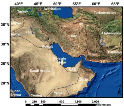
The study area is consisting of the western part of the Middle East, which includes the west and 94
southwest of Iran, Iraq, Saudi Arabia, Kuwait, Yemen, and the United Arab Emirates (see Fig. 1). 95
Most of these regions are located in the semi-arid and arid region and have a little annual rainfall. 96
There are many deserts in this area. Due to Shamal winds, the areas mentioned above are typically 97
experiencing dust in the spring and summer. 98
Fig. 1 The study area, the Middle East region around the Persian Gulf.
2.2. Earth Observations
99
2.2.1. MODIS Data 100
MODIS is a passive satellite sensor that provides data in the visible and infrared spectral domain, 101
including thermal infrared. Thermal bands of MODIS sensor, installed on Aqua and Terra satellites 102
launched in 1999 and 2002, is widely used for detecting dust in satellite images [55, 26]. MODIS 103
has 36 bands in the visible to thermal infrared spectrum (0.4 – 14.4 µm). From these bands, bands 104
1 and 2 have a 250-meter resolution, while bands 3 to 7 have 500-meter resolution, and bands 8 to 105
36 have 1 km of resolution [25]. Thermal bands have a spatial resolution of 1 km by 1 km. These 106
sensors are observing the entire surface of the planet Earth every day or two. Due to its extensive 107
spatial coverage and high temporal resolution, MODIS data are useful to track large-scale 108
phenomena and environmental changes. 109
In this study, we used MODIS level 1B images from both Aqua and Terra satellites. Daily 110
MODIS Level 1B calibrated radiance data of MODIS sensors with 1 Km resolution are available 111
through the NASA website, i.e., at http://ladsweb.nascom.nasa.gov/. Level1 B MODIS data are 112
calibrated, geo-referenced, and geometrically corrected [60]. Re-projection and resampling were 113
applied to the data using the MODIS conversion toolkit (MCTK). Moreover, Level 1B images 114
were converted to brightness temperature using the MCTK toolkit. A list of the bands used for 115
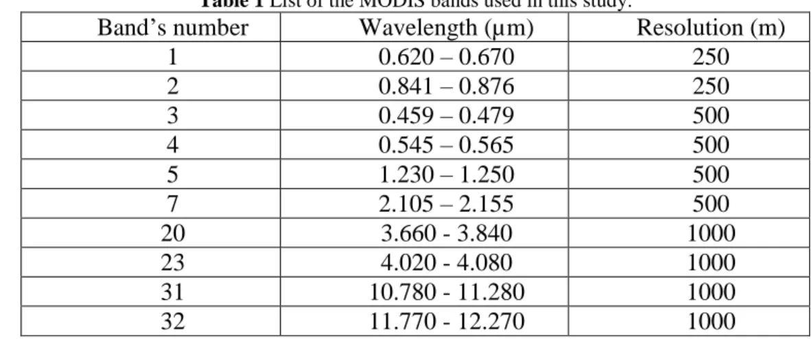
dust detection is presented in Table 1. 116
Table 1 List of the MODIS bands used in this study.
117 Resolution (m) Wavelength (µm) Band’s number 250 0.620 – 0.670 1 250 0.841 – 0.876 2 500 0.459 – 0.479 3 500 0.545 – 0.565 4 500 1.230 – 1.250 5 500 2.105 – 2.155 7 1000 3.660 - 3.840 20 1000 4.020 - 4.080 23 1000 10.780 - 11.280 31 1000 11.770 - 12.270 32 118
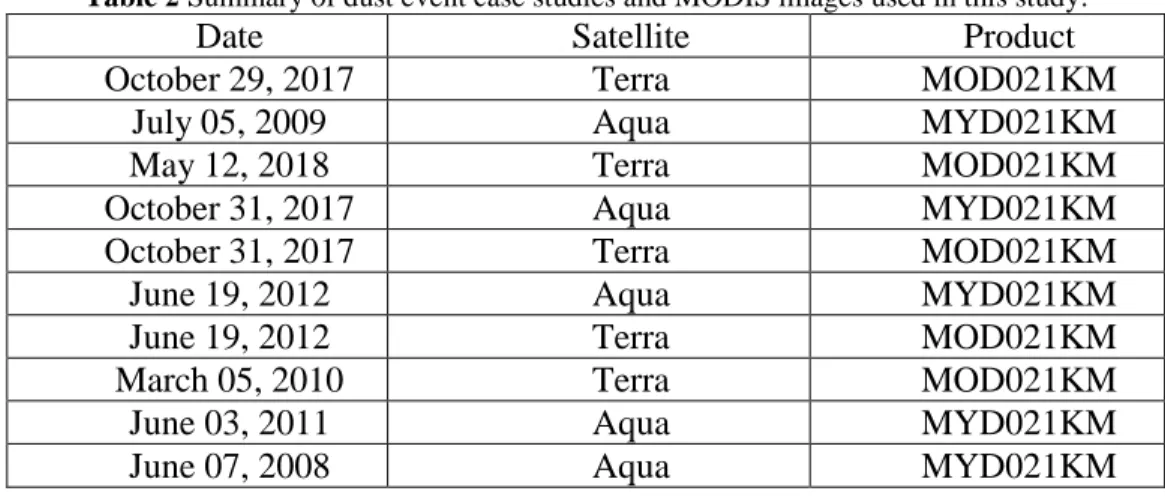
In this study, ten MODIS images from 2008 to 2018 were used to test and evaluate the proposed 119
dust detection algorithm. Table 2 presents a summary of these images. Three of these dust 120
events/images were used for sample data collection and threshold estimation, while the remaining 121
Table 2 Summary of dust event case studies and MODIS images used in this study. 123 Product Satellite Date MOD021KM Terra October 29, 2017 MYD021KM Aqua July 05, 2009 MOD021KM Terra May 12, 2018 MYD021KM Aqua October 31, 2017 MOD021KM Terra October 31, 2017 MYD021KM Aqua June 19, 2012 MOD021KM Terra June 19, 2012 MOD021KM Terra March 05, 2010 MYD021KM Aqua June 03, 2011 MYD021KM Aqua June 07, 2008 124 2.2.2. OMI Data 125
OMI is a nadir-viewing near-ultraviolet (UV) and visible charge-coupled device (CCD) 126
spectrometer aboard NASA’s Aura spacecraft with a resolution of 13 km by 24 km at nadir [61]. 127
Aura was launched on July 15, 2004. The OMI observes the Earth’s surface through two UV bands, 128
UV1 (270–314 nm) and UV2 (306–380 nm), and one visible band, VIS (350–500 nm). It is 129
essential to mention that the time difference between Aqua’s MODIS data and OMI was less than 130
15 min [62]. 131
The OMI can distinguish between different aerosol types, such as dust and smoke. It can 132
measure cloud pressure and coverage that can provide data to derive tropospheric ozone. 133
Considering the Lambert Equivalent Reflectivity (LER) assumption, the difference between the 134
measured and calculated radiance is described as the Aerosol Index [63]. The OMI near-UV 135
aerosol algorithm calculates the LER at 388 nm (i.e., R388∗ ) by assuming the atmosphere scattering
136
is purely Rayleigh [64]. Calculation of the UV Aerosol Index (UVAI) as follows: 137
UVAI = −100 log10[
I354obs
where I354obs is the radiation recorded by sensor and I354calc is calculated by assuming LER of R∗354. 138
Positive UVAI values indicate absorbing aerosol (carbonaceous aerosols, desert dust, 139
volcanic, etc.), While Negative values indicate non-absorbing aerosol. Near-zero values of UVAI 140
also indicate clouds, minimal aerosol, or other non-aerosol [64]. 141
In this study, OMI-Aura_L3-OMAERUV daily data was used for visual evaluation of the 142
dust detection model. 143
2.2.3. Ground Observations
144
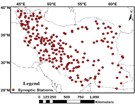
For performance evaluation of the proposed algorithm, the ground observations obtained from 212 145
synoptic stations, managed by Iran’s Meteorological Organization (IMO), which observe several 146
weather parameters every hour. These weather parameters were horizontal visibility and code 06. 147
Code 06 is a ground observation that measures the extensive and suspended dust particles, which 148
is not raised by the wind at or near the station at the time of observation. The remnants of dust 149
particles that came close to the observatory station due to sandstorms of trans-local origin and 150
reduced vertical visibility are also reported in Code 6. Due to the limited access to the synoptic 151
data from other countries, in this study, we used only the synoptic data of the IMO. It worths 152
mentioning that we used synoptic data at and near the time of satellite overpasses. Fig. 2 shows 153
the distribution of these synoptic stations across the whole country. 154
Fig. 2 The distribution of 212 synoptic stations utilized in this study.
2.3. Proposed Methodology
155
In this study, different steps were followed to identify the dust pixels from MODIS imagery. 156
Statistical analysis was first performed to find suitable bands and proper thresholds for better dust 157
detection. This analysis was based on the sampling of diverse objects (cloud, land, water, and dust 158
over different surfaces) in the MODIS images. Training data was used to extract the relevant 159
formula and thresholds. Three of the dust storms that occurred in 2012/06/19 (Aqua), 2011/06/03, 160
and 2010/03/05 are considered in this study to collect training data. After sampling and finding the 161
appropriate bands, the clouds were masked from the image. The next step was to identify water 162
bodies. Finally, using two separate methods, the dust was detected over water and land. The 163
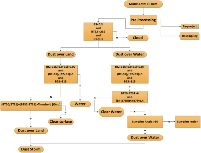
flowchart of the proposed approach is shown in Fig. 3. 164
To implement the proposed algorithm, we need to calculate the brightness temperature 165
of thermal bands. The brightness temperature is the temperature of a blackbody that emits the same 166
intensity when viewed with the same detector. The amount of radiation emitted by a black body 167
depends on its temperature, and is defined by Planck’s Law: 168
B(λ, T) = 2hc
2λ−5
exp (kTλhc ) − 1 (2)
where B(λ,T) is the Planck function at wavelength λ(m), T is brightness temperature, c=2.99×10⁸
169
m s-1 is the speed of light, h=6.626×10⁻³⁴ m2 kg s-1 is the Planck’s constant, and k=1.38×10⁻²³ J K
-170
1 is the Boltzmann’s constant. Using this equation, the temperature can be derived as follows:
171
T = hc
λkln (1 + 2hc2 Lλ5)
(3)
where L is the radiance value for a given pixel. 172
Fig. 3 The proposed dust detection approach.
2.3.1. Threshold estimation 173
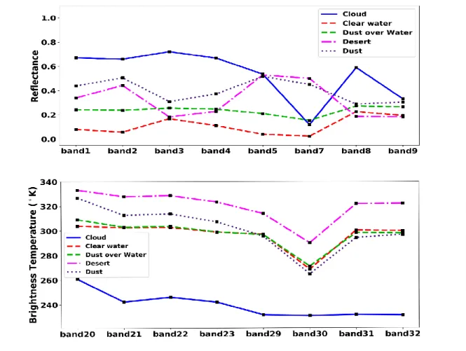
Modeling of the spectral behavior of different objects was performed based on all the MODIS 174
bands. Then, useful(valuable) bands were selected for each object. Approximately 10,000 pixels 175
of each class in three images were sampled for five classes, and then, their statistical parameters 176
were calculated. Fig. 4 represents the extracted spectral signatures of clouds, clear water, dust over 177
water, desert, and dust over land. 178
Fig. 4Spectral Reflectance (top), and Brightness Temperature (bottom) signatures of different objects.
By calculating the statistical parameters and thresholds, the proposed indices were modeled and 179
applied to the images. Fig. 5 shows the results in the box plots. A box plot displays the distribution 180
of quantitative data so that it facilitates comparisons between variables. The box shows the 181
where R0.645 µm , R0.858 µm , and R1.24 µm is the reflectance of band 1, 2, and 5.
188
Considering all datasets and bands, we noticed that the brightness temperature difference 189
between band 20 and band 31, as well as a relationship between band 4 and band 7 is suitable to 190
detect dust over water: 191
𝐵𝑇𝐷3.7−11 μm= 𝐵𝑇3.7 μm− 𝐵𝑇11 μm , (6)
𝑅4,7=
𝑅0.545 μm− 𝑅2.105 μm
𝑅0.545 μm+ 𝑅2.105 μm (7)
where R0.545 µm and R2.105 µm are reflectance values in bands 4 and 7. BT3.7 µm and BT11 µm are the
192
brightness temperature of bands 20 and 31. 193
𝑁𝐷𝑊𝐼 =𝑅0.858 μm− 𝑅1.24 μm
𝑅0.858 μm+ 𝑅1.24 μm (4)
𝑁𝐷𝑉𝐼 =𝑅0.858 μm− 𝑅0.645 μm
2.3.2. Clouds Masking 194
As shown in the flowchart (Fig. 3), the first step in implementing the proposed method is to mask 195
clouds in the images. Clouds exhibit a much lower value of brightness temperature than other 196
objects (Fig. 4-b). Brightness temperature is not capable of detecting thin clouds alone. Song et 197
al. [65] suggested a method for mask clouds using reflection of band 1 (0.66 µm)-because of 198
clouds’ high reflection in this band-and brightness temperature of band 32 (12 µm). Unfortunately, 199
after applying these formulas, clouds are not entirely masked, therefore, besides the mentioned 200
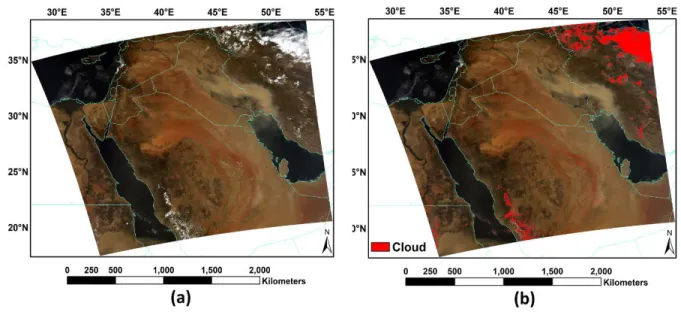
bands, band 3 is utilized for cloud detection because of high reflection in this band (Fig. 4-a). Fig. 201
6-a depicts the result for the cloud mask of the proposed method on the image of the dust event in 202
2012. 203
Fig. 6 Result of cloud masking (a), and the MODIS RGB image (b).
2.3.3. Water Delamination 204
The spectral behavior of thin dust over water differs from that of thick dust. Conventional strategies 205
cannot detect thin dust over water. Accordingly, we mapped the water bodies in the image. Using 206
spectral and statistical analysis, three formulas were selected for the identification of water bodies. 207
The amount of NDWI (Eq. (4)) to detect water is greater than zero (Fig. 5-c) [66, 67]. As 208
well as, the value of NDVI (Eq. (5)) is less than zero, but According to Fig. 5-a, if thin dust was 209
presented above the water bodies, the value of NDVI will be slightly higher than zero accordingly. 210
Therefore, the threshold is set to a value above zero. Moreover, the brightness temperature of band 211
23 was used to detect water bodies with respect to the difference in value with other objects (Fig. 212
4-b and Fig. 5-d). 213
Fig. 7-a showed the results for the water bodies’ delamination of the proposed method 214
implemented on the image of the dust event in 2012. 215
transparent and opaque water pixels. Considering the statistical analysis of the transparent and 220
opaque water pixels, BTD3.7-11 µm and R4,7 (Eq. (6) and (7)) were applied to distinguish these two
221
classes. MODIS Aqua and Terra images have sun-glint over water. In order to remove this effect, 222
we detect dust for the sun-glint free region (with a sun-glint angle greater than 30 degrees) [68]. 223
2.3.5. Dust detection over the land surface 224
The main challenge in detecting dust using satellite data is the separation of the spectral signal of 225
dust from the surface of the Earth and the cloud, and this is especially challenging for bright 226
surfaces [41, 42]. Due to similar reflectivity of dust particles and deserts in the visible bands, dust 227
storm detection in the Middle East region is more complicated. Furthermore, using a single thermal 228
band cannot distinguish between dust and other objects. As a solution to these limitations, using a 229
combination of thermal, visible, and infrared bands from MODIS imagery can efficiently detect 230
the dust [44, 24]. 231
Ackerman [43, 44] used the brightness temperature difference of band 20 (3.66-3.84 µm) and band 232
31 (11.28 – 1.78 µm), i.e., BTD 3.75-11 µm, and difference of band 32 (12.22 – 11.77 µm) and band
233
31, i.e., BTD12-11 µm. Although BTD 3.75-11 µm can efficiently make a distinction between dust and
234
ground surface, it cannot discriminate cloud and dust [44]. 235
Based on the analysis of different bands, as well as the statistical analysis of different 236
classes, we found that the brightness temperature of bands 20, 31, and 32 is suitable for dust 237
detection over the land surfaces. These bands have been used in various studies to detect dust [43, 238
44]. For this reason, we have found two relationships to detect dust on land cover areas (Eq. (8) 239 and (9)). 240 𝐵𝑎𝑛𝑑 𝑅𝑎𝑡𝑖𝑜3.7𝜇𝑚−11𝜇𝑚= BT3.7 μm BT11 μm (8) BTD11−12= BT11 μm− BT12 μm (9)
where BT3.7 µm , BT11 µm and BT12 µm are the brightness temperature of band 20, 31, and 32.
241
The 2012’s satellite image was selected to perform this analysis. The results of these two 242
equations are shown in Fig. 8-a and Fig. 8-b. Using these two equations separately, we cannot 243
extract dust entirely from the image. For this reason, training regions were used to analyse these 244
Improved Dust Index = (BT3.7 μm BT11 μm
)
(BT12 μm−BT11 μm) (10)
The threshold for this index was calculated using the Otsu algorithm [69]. This algorithm is based 249
on an iterating procedure through all the possible thresholds. It calculates a measure of spread on 250
each side of the threshold and ultimately finds the optimal threshold values with the minimum 251
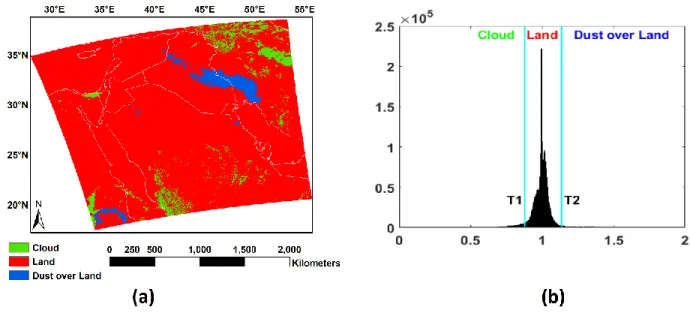
inter- or the maximum intera- class variance. The dust index (Eq. (10)) was applied to the dust 252
event images, and the result was classified into three classes of dust, land, and cloud (Fig. 9). The 253
two threshold values (T1 and T2) are generally not constant and vary based on the season of 254
occurring dust storms. 255
Fig. 9 Result of classification of the improved index with Otsu’s thresholding (a), and the histogram of the image (b).
3. Results and Discussion 256
The proposed algorithm was applied and evaluated on ten dust occurrences from 2008 to 257
2018. Fig. 10-b, Fig. 11-b, and Fig. 12-b show the results of the proposed algorithm 258
implementation on test images. In Fig. 10-b, it is apparent that the clouds masked well. Although 259
there are many clouds in this image, the algorithm has been able to detect dust with decent 260
accuracy. Thin dust over the water was also detected well. In the 2011 dust event, the algorithm 261
has detected many dust particles over the water. The clouds are relatively well masked in the image 262
(Fig. 11-b). In the 2012 dust event, water bodies were identified well, and thin and thick dust over 263
them was detected with reasonable accuracy. Clouds were masked well. Finally, dust over the land 264
was detected (Fig. 12-b). 265
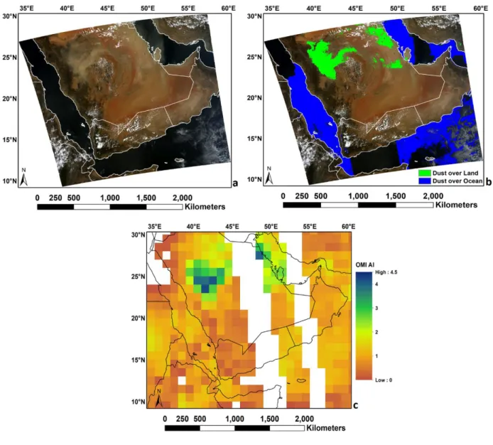
Fig. 11 Results of the proposed algorithm (a), MODIS RGB images (b), and OMI AI (c) obtained on June 3 2011.
Bin Abdulwahed, Dash and Roberts [5] evaluated various dust detection algorithms in the Middle 266
East [5]. Their results showed that the Middle East Dust Index (MEDI) had difficulty 267
distinguishing dust from dark and deserts regions. Also, their results showed that the brightness 268
temperature difference is not capable of distinguishing dust from the bright surfaces well. They 269
stated that the Normalized Difference Dust Index (NDDI) was more agree with the AERONET 270
among the indicators they examined. 271
using the brightness temperature is to distinguish dusty pixels from the cloud. Because of the low 278
spatial resolution of MODIS, thin clouds in pixels may have the same behavior of dust in the 279
image. Appropriate cloud masking helped us to identify dust pixels better and might significantly 280
reduce the number of false alarm pixels; in other words, pixels that were not dust but identified by 281
the algorithm as dust. The next significant limitation of dust detection algorithms is the inability 282
to detect dust over water bodies. It is challenging to identify thin dust pixels over water bodies 283
with the brightness temperature merely. We need to detect thin dust over these areas with a separate 284
method. Fortunately, in the proposed method, we were able to identify the dust smoothly by using 285
statistical analysis. 286
Furthermore, distinguishing between dust pixels and bright surfaces such as deserts, which 287
are abundant in the Middle East, is another challenge. Accurate threshold estimation in these areas 288
is essential. We were able to overcome this problem to an acceptable level by automatically finding 289
the threshold. Moreover, Lower threshold values in the improved index to detect dust over the land 290
surface may cause problems between dust and desert. The proposed algorithm has a higher 291
capability to distinguish between dust and other objects. 292
3.1. Validation
293
There are several ways to evaluate dust detection algorithms. In this paper, three separate panels 294
were created to evaluate the proposed method for each three dust events. In each case, the results 295
of the proposed method visually evaluated with MODIS RGB images where red, green, and blue 296
are band 1, band 4, and band 3, respectively. Also, the results visually evaluated with OMI AI 297
products. Although the OMI resolution is lower than the MODIS resolution, these products can 298
indicate the intensity and location of the dust particles. Finally, the results of the method were 299
3.1.1. Visual evaluation of MODIS’s dust detection 301
The results of the proposed algorithm are in good accordance with MODIS RGB images. Although 302
MODIS images can be good at visually detecting thick dust, they have poor performance at 303
detecting dust, especially in desert areas. 304
In the 2010 dust event, although the dust on the water and land is thin, the algorithm has 305
been able to identify it relatively well (Fig. 10 a and b). However, a significantly lower threshold 306
may be able to detect dust over the land more accurately. In the 2011 dust event, it is challenging 307
to identify dust pixels over water and land visually. In this image, although the cloud is present in 308
the image, the number of false alarms is near zero (Fig. 11 a and b). In the 2012 dust event, many 309
south-western synoptic stations of IMO recorded a reduction in visibility to less than 1km. There 310
is also some dust in the middle part of the image, but it cannot be seen in the RGB image (Fig. 12 311
a and b). There are some clouds in this image, but the number of false alarm pixels is deficient. 312
3.1.2. Visual companion with OMI-AI 313
OMI-AI for three dust events are presented in Fig. 10-c, Fig. 11-c, and Fig. 12-c. In the 2012 dust 314
event, the results of the OMI-AI measurement are very consistent with the output of the proposed 315
algorithm over water. An examination of the results of the proposed algorithm and images of OMI-316
AI shows that our method was able to perform better for the AI larger than 1.7. In the 2011 dust 317
time difference, and the dynamic behavior of the dust, the results of the algorithm may be different 323 from OMI. 324 3.1.3. Accuracy assessment 325
Because some of the synoptic stations were exterior of the studied region for dust detection, the 326
analytical evaluation of the proposed algorithm was limited to the only overlapped areas. 327
Horizontal visibility is a suitable parameter for the identification of the days that dust storms are 328
occurred [26]. Therefore, 3-hourly synoptic data (i.e., horizontal visibility and code 06) records 329
from 212 synoptic stations used to evaluate the proposed method. It should be noted that the 330
maximum time difference between the MODIS images and the synoptic data was about 15 331
minutes. 332
For classification assessment, a confusion matrix is widely used to evaluate the 333
performance of the algorithm. The confusion matrix, for a binary classification case, is a table with 334
two rows and two columns. It reports the number of true positives (TP), true negatives (TN), false 335
positives (FP), and false negatives (FN). For each of ten dust events, image pixels were classified 336
into two classes of “dust” and “no dust.” Here, TP represents the number of pixels where both 337
synoptic data and proposed algorithm indicate the presence of “dust.” FP is the number of pixels 338
where synoptic data indicates “no dust.” FN is the number of pixels where synoptic data indicates 339
“dust,” but the proposed algorithm indicates “no dust.” Finally, the variable TN represents the 340
number of pixels where both synoptic and proposed algorithms indicate “no dust.” 341
Three statistical metrics, including accuracy, True Positive Rate (TPR), and False 342
Discovery Rate (FDR), were calculated using the following equations and used for accuracy 343
assessment. 344
Accuracy = 𝑇𝑃 + 𝑇𝑁 𝑇𝑃 + 𝐹𝑃 + 𝐹𝑁 + 𝑇𝑁 (11) TPR = 𝑇𝑃 𝑇𝑃 + 𝐹𝑁 (12) FDR = 𝐹𝑃 𝑇𝑃 + 𝐹𝑃 (13)
The performance of the proposed algorithm is evaluated using contingency Table 3. 345
Table 3 The results of validation with synoptic data
346 Date Accuracy TPR FDR 29 Oct 2017 0.76 0.74 0.30 05 Jul 2009 0.78 0.77 0.28 12 May 2018 0.77 0.76 0.28 31 Oct 2017 0.82 0.72 0.29 31 Oct 2017 0.81 0.73 0.29 19 Jun 2012 0.83 0.71 0.27 07 Jun 2008 0.81 0.78 0.31 Overall 0.80 0.74 0.29
As shown in Table 3, the overall accuracy for the dust detection algorithm was ~80 %. TPR and 347
Level-1B data. The output dust maps were visually compared with MODIS RGB images and OMI-353
AI products as well as, the results of the proposed method were evaluated with observations from 354
several synoptic ground stations of the Iranian meteorological organization. In total, three dust 355
events were selected to collect sampling data and seven dust events to evaluate the efficiency of 356
the proposed method. The overall accuracy of the dust detection algorithm was about 81%. The 357
results showed that this model has acceptable accuracy for dust detection over both water and land 358
areas. In particular, in contrast to the previous models, the proposed method was capable of 359
detecting thin dust on the water. Low-density dust is not always visible in MODIS images due to 360
its low spatial resolution. Therefore, there may be an uncertainty of detection over the 361
corresponding areas. As a solution, higher spatial and temporal resolution satellite imagery can 362
help better detection of dust in our future research. The proposed algorithm is planned to be 363
implemented in the Google Earth Engine and to be served as the basis of a Spatial Support Decision 364
System for various end-users. 365
References 366
1. L. San-Chao et al., “Detection of dust storms by using daytime and nighttime multi-spectral 367
modis images,”2006 IEEE International Symposium on Geoscience and Remote 368
Sensing,294-296,Ieee,2006),[doi:10.1109/igarss.2006.80].
369
2. A. S. Goudie and N. J. Middleton, Desert dust in the global system, Springer Science & 370
Business Media, (2006), [doi:10.1007/3-540-32355-4]. 371
3. H. M. El-Askary et al., ”A multisensor approach to dust storm monitoring over the nile 372
delta,” IEEE Transactions on Geoscience and Remote Sensing, 41, 10, 2386-2391, (2003), 373
[doi:10.1109/tgrs.2003.817189]. 374
4. M. F. Yassin, S. K. Almutairi and A. Al-Hemoud, ”Dust storms backward trajectories' and 375
source identification over kuwait,” Atmospheric research, 212, 158-171, (2018), 376
[doi:10.1016/j.atmosres.2018.05.020]. 377
5. A. Bin Abdulwahed, J. Dash and G. Roberts, ”An evaluation of satellite dust-detection 378
algorithms in the middle east region,” International journal of remote sensing, 40, 4, 1331-379
1356, (2019), [doi:10.1080/01431161.2018.1524589]. 380
6. P. Jafary, A. Zandkarimi and M. Jannati, ”Annual monitoring of dust storm in iran and 381
adjacent areas using modis images (1396 and 1397 hijri shamsi),” International Archives 382
of the Photogrammetry, Remote Sensing & Spatial Information Sciences, (2019),
383
[doi:10.5194/isprs-archives-xlii-4-w18-565-2019]. 384
7. M. Bennell, J. Leys and H. Cleugh, ”Sandblasting damage of narrow-leaf lupin (lupinus 385
angustifolius l.): A field wind tunnel simulation,” Soil Research, 45, 2, 119-128, (2007), 386
[doi:10.1071/sr06066]. 387
8. A. Chedin, V. Capelle and N. Scott, ”Detection of iasi dust aod trends over sahara: How 388
many years of data required?,” Atmospheric research, 212, 120-129, (2018), 389
[doi:10.1016/j.atmosres.2018.05.004]. 390
9. A. Al-Hemoud et al., ”Socioeconomic effect of dust storms in kuwait,” Arabian Journal of 391
Geosciences, 10, 1, 18, (2017), [doi:10.1007/s12517-016-2816-9].
392
10. T. X.-P. Zhao, S. Ackerman and W. Guo, ”Dust and smoke detection for multi-channel 393
imagers,” Remote Sensing, 2, 10, 2347-2368, (2010), [doi:10.3390/rs2102347]. 394
11. P. Zhang et al., ”Identification and physical retrieval of dust storm using three modis 395
thermal ir channels,” Global and Planetary Change, 52, 1-4, 197-206, (2006), 396
[doi:10.1016/j.gloplacha.2006.02.014]. 397
12. H. El-Askary et al., “Introducing new approaches for dust storms detection using remote 398
sensing technology,”IGARSS 2003. 2003 IEEE International Geoscience and Remote 399
Sensing Symposium. Proceedings (IEEE Cat. No.
03CH37477),2439-400
2441,IEEE,2003),[doi:10.1109/igarss.2003.1294468]. 401
13. L. Perez et al., ”Saharan dust, particulate matter and cause-specific mortality: A case-402
crossover study in barcelona (spain),” Environ Int, 48, 150-155, (2012), 403
[doi:10.1016/j.envint.2012.07.001]. 404
14. D. W. Griffin and C. A. Kellogg, ”Dust storms and their impact on ocean and human health: 405
Dust in earth’s atmosphere,” EcoHealth, 1, 3, 284-295, (2004), [doi:10.1007/s10393-004-406
0120-8]. 407
15. B. Laurent et al., ”Simulation of the mineral dust emission frequencies from desert areas 408
of china and mongolia using an aerodynamic roughness length map derived from the 409
polder/adeos 1 surface products,” Journal of Geophysical Research: Atmospheres, 110, 410
D18, (2005), [doi:10.1029/2004jd005013]. 411
16. A. Zandkarimi and P. Fatehi, ”Dust storm detection using modis data over the middle east,” 412
The International Archives of Photogrammetry, Remote Sensing and Spatial Information
413
Sciences, 42, 1147-1151, (2019), [doi:10.5194/isprs-archives-xlii-4-w18-1147-2019].
414
17. M. H. Saeifar and B. Alijani, ”Detection of dust storm origins in the middle east by 415
remotely sensed data,” Journal of the Indian Society of Remote Sensing, 47, 11, 1883-1893, 416
(2019), [doi:10.1007/s12524-019-01030-5]. 417
22. K. Schepanski, I. Tegen and A. Macke, ”Comparison of satellite based observations of 428
saharan dust source areas,” Remote Sensing of Environment, 123, 90-97, (2012), 429
[doi:10.1016/j.rse.2012.03.019]. 430
23. H. El-Askary et al., ”Dust storms detection over the indo-gangetic basin using multi sensor 431
data,” Advances in Space Research, 37, 4, 728-733, (2006),
432
[doi:10.1016/j.asr.2005.03.134]. 433
24. T. Takashima and K. Masuda, ”Emissivities of quartz and sahara dust powders in the 434
infrared region (7–17 μ),” Remote Sensing of Environment, 23, 1, 51-63, (1987), 435
[doi:10.1016/0034-4257(87)90070-8]. 436
25. P. D. Kunte and M. Aswini, ”Detection and monitoring of super sandstorm and its impacts 437
on arabian sea—remote sensing approach,” Atmospheric Research, 160, 109-125, (2015), 438
[doi:10.1016/j.atmosres.2015.03.003]. 439
26. M. C. Baddock, J. E. Bullard and R. G. Bryant, ”Dust source identification using modis: A 440
comparison of techniques applied to the lake eyre basin, australia,” Remote Sensing of 441
Environment, 113, 7, 1511-1528, (2009), [doi:10.1016/j.rse.2009.03.002].
442
27. M. J. Butt, M. E. Assiri and M. A. Ali, ”Assessment of aod variability over saudi arabia 443
using modis deep blue products,” Environmental pollution, 231, 143-153, (2017), 444
[doi:10.1016/j.envpol.2017.07.104]. 445
28. I. Gunaseelan, B. V. Bhaskar and K. Muthuchelian, ”The effect of aerosol optical depth on 446
rainfall with reference to meteorology over metro cities in india,” Environ Sci Pollut Res 447
Int, 21, 13, 8188-8197, (2014), [doi:10.1007/s11356-014-2711-4].
448
29. S. Gehlot, P. J. Minnett and D. Stammer, ”Impact of sahara dust on solar radiation at cape 449
verde islands derived from modis and surface measurements,” Remote Sensing of 450
Environment, 166, 154-162, (2015), [doi:10.1016/j.rse.2015.05.026].
451
30. S. S. Park et al., ”Combined dust detection algorithm by using modis infrared channels 452
over east asia,” Remote sensing of environment, 141, 24-39, (2014), 453
[doi:10.1016/j.rse.2013.09.019]. 454
31. S. Janugani et al., “Directional analysis and filtering for dust storm detection in noaa-avhrr 455
imagery,”Algorithms and Technologies for multispectral, hyperspectral, and ultraspectral 456
imagery XV,73341G,International Society for Optics and 457
Photonics,2009),[doi:10.1117/12.819070]. 458
32. A. T. Evan, A. K. Heidinger and M. J. Pavolonis, ”Development of a new over‐water 459
advanced very high resolution radiometer dust detection algorithm,” International Journal 460
of Remote Sensing, 27, 18, 3903-3924, (2006), [doi:10.1080/01431160600646359].
461
33. M. Rezaei et al., ”Analysis of spatio-temporal dust aerosol frequency over iran based on 462
satellite data,” Atmospheric Pollution Research, 10, 2, 508-519, (2019), 463
[doi:10.1016/j.apr.2018.10.002]. 464
34. Y. Yang et al., ”A simplified suomi npp viirs dust detection algorithm,” Journal of 465
Atmospheric and Solar-Terrestrial Physics, 164, 314-323, (2017),
[doi:10.5270/esa-466
91oxxtk]. 467
35. P. Alpert et al., ”Vertical distribution of saharan dust based on 2.5-year model predictions,” 468
Atmospheric Research, 70, 2, 109-130, (2004), [doi:10.1016/j.atmosres.2003.11.001].
469
36. B. Chen et al., ”Detection of dust aerosol by combining calipso active lidar and passive iir 470
measurements,” Atmospheric Chemistry & Physics Discussions, 10, 2, (2010), 471
[doi:10.5194/acp-10-4241-2010]. 472
37. A. Moridnejad, N. Karimi and P. A. Ariya, ”A new inventory for middle east dust source 473
points,” Environ Monit Assess, 187, 9, 582, (2015), [doi:10.1007/s10661-015-4806-x]. 474
38. Y. J. Kaufman et al., ”The effect of smoke, dust, and pollution aerosol on shallow cloud 475
development over the atlantic ocean,” Proc Natl Acad Sci U S A, 102, 32, 11207-11212, 476
(2005), [doi:10.1073/pnas.0505191102]. 477
39. D. Tanré et al., ”Remote sensing of aerosol properties over oceans using the modis/eos 478
spectral radiances,” Journal of Geophysical Research: Atmospheres, 102, D14, 16971-479
16988, (1997), [doi:10.1029/96jd03437]. 480
40. A. Sayer et al., ”Validation and uncertainty estimates for modis collection 6 “deep blue” 481
aerosol data,” Journal of Geophysical Research: Atmospheres, 118, 14, 7864-7872, (2013), 482
[doi:10.1002/jgrd.50600]. 483
41. N. C. Hsu et al., ”Deep blue retrievals of asian aerosol properties during ace-asia,” IEEE 484
Transactions on Geoscience and Remote Sensing, 44, 11, 3180-3195, (2006),
485
[doi:10.1109/tgrs.2006.879540]. 486
42. N. C. Hsu et al., ”Aerosol properties over bright-reflecting source regions,” IEEE 487
Transactions on Geoscience and Remote Sensing, 42, 3, 557-569, (2004),
488
[doi:10.1016/s0021-8502(98)90762-5]. 489
43. S. A. Ackerman, ”Remote sensing aerosols using satellite infrared observations,” Journal 490
of Geophysical Research: Atmospheres, 102, D14, 17069-17079, (1997), 491
[doi:10.1029/96jd03066]. 492
44. ---, ”Using the radiative temperature difference at 3.7 and 11 μm to tract dust outbreaks,” 493
Remote Sensing of Environment, 27, 2, 129-133, (1989),
[doi:10.1016/0034-494
4257(89)90012-6]. 495
45. H. Yue et al., ”The brightness temperature adjusted dust index: An improved approach to 496
detect dust storms using modis imagery,” International journal of applied earth 497
observation and geoinformation, 57, 166-176, (2017), [doi:10.1016/j.jag.2016.12.016].
498
46. X. Hao and J. J. Qu, ”Saharan dust storm detection using moderate resolution imaging 499
spectroradiometer thermal infrared bands,” Journal of Applied Remote Sensing, 1, 1, 500
013510, (2007), [doi:10.1117/1.2740039]. 501
47. N. Karimi et al., ”Comparison of dust source identification techniques over land in the 502
middle east region using modis data,” Canadian Journal of Remote Sensing, 38, 5, 586-503
599, (2012), [doi:10.5589/m12-048]. 504
48. Y. Liu and R. Liu, “A thermal index from modis data for dust detection,”2011 IEEE 505
International Geoscience and Remote Sensing
Symposium,3783-506
3786,IEEE,2011),[doi:10.1109/igarss.2011.6050054]. 507
53. S. Miller, ”A consolidated technique for enhancing desert dust storms with modis,” 519
Geophysical Research Letters, 30, 20, (2003), [doi:0.1029/2003gl018279].
520
54. E. El-ossta, R. Qahwaji and S. S. Ipson, ”Detection of dust storms using modis reflective 521
and emissive bands,” IEEE Journal of Selected Topics in Applied Earth Observations and 522
Remote Sensing, 6, 6, 2480-2485, (2013), [doi:10.1109/jstars.2013.2248131].
523
55. S. Albugami et al., ”Evaluating modis dust-detection indices over the arabian peninsula,” 524
Remote Sensing, 10, 12, 1993, (2018), [doi:10.3390/rs10121993].
525
56. M. Boroughani et al., ”Application of remote sensing techniques and machine learning 526
algorithms in dust source detection and dust source susceptibility mapping,” Ecological 527
Informatics, 56, 101059, (2020), [doi:10.1016/j.ecoinf.2020.101059].
528
57. P. Ginoux et al., ”Global‐scale attribution of anthropogenic and natural dust sources and 529
their emission rates based on modis deep blue aerosol products,” Reviews of Geophysics, 530
50, 3, (2012), [doi:10.1029/2012rg000388]. 531
58. F. Khoshakhlagh, M. Najafi and M. Samadi, ”An analysis on synoptic patterns of 532
springtime dust occurrence in west of iran,” (2012), [doi:10.1256/qj.05.109]. 533
59. H. K. H. Furman, ”Dust storms in the middle east: Sources of origin and their temporal 534
characteristics,” Indoor and Built Environment, 12, 6, 419-426, (2003), 535
[doi:10.1177/1420326x03037110]. 536
60. L. Han et al., ”An enhanced dust index for asian dust detection with modis images,” 537
International journal of remote sensing, 34, 19, 6484-6495, (2013), 538
[doi:10.1080/01431161.2013.802055]. 539
61. R. Jafari and M. Malekian, ”Comparison and evaluation of dust detection algorithms using 540
modis aqua/terra level 1b data and modis/omi dust products in the middle east,” 541
International Journal of Remote Sensing, 36, 2, 597-617, (2015), 542
[doi:10.1080/01431161.2014.999880]. 543
62. K. Sun, Q. Su and Y. Ming, ”Dust storm remote sensing monitoring supported by modis 544
land surface reflectance database,” Remote Sensing, 11, 15, 1772, (2019), 545
[doi:10.3390/rs11151772]. 546
63. D. Kaskaoutis et al., ”The aura–omi aerosol index distribution over greece,” Atmospheric 547
Research, 98, 1, 28-39, (2010), [doi:10.1109/igarss.2011.6050054].
548
64. O. Torres et al., ”Aerosols and surface uv products from ozone monitoring instrument 549
observations: An overview,” 112, D24, (2007), 550
65. X. Song, Z. Liu and Y. Zhao, “Cloud detection and analysis of modis image,”IGARSS 551
2004. 2004 IEEE International Geoscience and Remote Sensing
Symposium,2764-552
2767,IEEE,2004),[doi:10.1029/2004jd005013]. 553
66. H. J. I. j. o. r. s. Xu, ”Modification of normalised difference water index (ndwi) to enhance 554
open water features in remotely sensed imagery,” 27, 14, 3025-3033, (2006), 555
67. S. K. J. I. j. o. r. s. McFeeters, ”The use of the normalized difference water index (ndwi) in 556
the delineation of open water features,” 17, 7, 1425-1432, (1996), 557
68. P. Ciren and S. J. J. o. G. R. A. Kondragunta, ”Dust aerosol index (dai) algorithm for 558
modis,” 119, 8, 4770-4792, (2014), 559
69. N. J. I. t. o. s. Otsu, man, and cybernetics, ”A threshold selection method from gray-level 560
histograms,” 9, 1, 62-66, (1979), 561