1
1
Verification of Regional Deterministic Precipitation Analysis products using snow data
1
assimilation for application in meteorological network assessment in sparsely gauged
2
Nordic basins
3
Kian Abbasnezhadi1,2,*,† Alain N. Rousseau1, Étienne Foulon1, and Stéphane Savary1
4
1 Institut National de la Recherche Scientifique, Centre eau terre et environnement, Québec,
5
Québec, Canada
6
2 YukonU Research Centre, Yukon University, Whitehorse, Yukon, Canada
7
* Corresponding author: Climate Research Division, Science and Technology Branch,
8
Environment and Climate Change Canada, 4509 Dufferin St., Toronto, ON M3H 5T4
9
† Former address: Institut National de la Recherche Scientifique, Centre Eau Terre
11
Environnement (INRS-ETE), 490 rue de la Couronne, Québec, QC G1K 9A9, Canada.
12
Abstract
13
Sparse precipitation information can result in uncertainties in hydrological modelling
14
practices. Precipitation observation network augmentation is one way to reduce the uncertainty.
15
Meanwhile, in basins with snowpack-dominated hydrology, in the absence of a high-density
16
precipitation observation network, assimilation of in situ and remotely sensed measurements of
17
snowpack state variables can also provide the possibility to reduce flow estimation uncertainty.
18
Similarly, assimilation of existing precipitation observations into gridded numerical precipitation
19
products can alleviate the adverse effects of missing information in poorly instrumented basins. In
20
Canada, the Regional Deterministic Precipitation Analysis (RDPA) data from the Canadian
21
Precipitation Analysis (CaPA) system have been increasingly applied for flow estimation in
22
sparsely gauged Nordic basins. Moreover, CaPA-RDPA data have also been applied to establish
23
observational priorities for augmenting precipitation observation networks. However, the accuracy
24
of the assimilated data should be validated before being applicable in observation network
25
assessment. The assimilation of snowpack state variables has proven to significantly improve
26
streamflow estimates, and therefore, it can provide the benchmark against which the impact of
27
assimilated precipitation data on streamflow simulation can be compared. Therefore, this study
28
introduces a parsimonious framework for performing a proxy-validation of the precipitation
29
assimilated products through the application of snow assimilation in physically-based hydrologic
30
models. This framework is demonstrated to assess the observation networks in three boreal basins
31
in Yukon, Canada. The results indicate that in most basins, the gridded analysis products generally
32
enjoyed the level of accuracy required for accurate flow simulation and therefore were applied in
33
the meteorological network assessment in those cases.
1. Introduction
35
The spatio-temporal representativeness of liquid and solid precipitation data is among the
36
most crucial factors in every flow simulation practice. Sporadic meteorological observations,
37
among other data constraints, can result in uncertainties in many hydrological modelling practices
38
performed for flow and inflow forecasting. This is also the case with the HYDROTEL system
39
(Bouda et al., 2012; Bouda et al., 2014; Fortin et al., 2001a; Turcotte et al., 2003; Turcotte et al.,
40
2007) set up for the watersheds in Yukon in northwestern Canada, where data constraints due to
41
sparsely distributed precipitation information in major basins of interest have adversely affected
42
the performance of the modelling system. Therefore, it is obvious that augmenting the precipitation
43
observation network could greatly reduce the uncertainty involved with meteorological forcing.
44
In many forecasting centers around the globe where streamflow simulation is performed in
45
basins with a hydrology dominated by snowpack melt during spring freshet, in the absence of a
46
high-density precipitation observation network, assimilation of in situ and remotely sensed
47
measurements of snowpack state variables has become increasingly important for accurate flow
48
estimation (Helmert et al., 2018). Li et al. (2019) have shown that in snow dominated basins, where
49
the meteorological uncertainty during the forecast period is significant (which is the case for
50
sparsely gauged networks), reinitializing the model based on observed snow water equivalent
51
(SWE) information can significantly improve streamflow forecasts. Similarly, in the absence of a
52
high-density precipitation observation network, assimilation of snowpack state variables can
53
provide the possibility to handle different sources of uncertainty by merging the value of observed
54
information into the model in order to correct the effects of model errors and improve forecasting
55
capabilities (Turcotte et al., 2010).
SWE reinitialization through various data assimilation (DA) approaches has been proven to
57
be an effective approach to improve the degree of agreement between the simulated and observed
58
discharge values (see, e.g., Clark et al., 2006; De Lannoy et al., 2012; Leisenring and Moradkhani,
59
2011; Nagler et al., 2008; Liu et al., 2013; Saloranta, 2016). Several DA techniques are available
60
for updating snow state variables, including direct insertion (Liston et al., 1999), Cressman
61
interpolation (Drusch et al., 2004), optimal interpolation (Brasnett, 1999), nudging (Boni et al.,
62
2010), particle filtering (Arulampalam et al., 2002), and various types of Kalman filtering
63
approaches with different levels of complexity (Gelb, 1974; Miller et al., 1994; Moradkhani, 2008;
64
Evensen, 1994). Among these approaches, Kalman filtering, and its Monte Carlo-based
65
implementation, the Ensemble Kalman Filtering (EnKF) approach, have been widely applied in
66
different hydrological modelling studies (see, e.g., Andreadis et al., 2006; Clark et al., 2006; De
67
Lannoy et al., 2012; Durand and Margulis, 2008; Huang et al., 2017; Magnusson et al., 2014;
68
Piazzi et al., 2018; Slater and Clark, 2006; Su et al., 2008).
69
Currently, to gain a proper insight into short-term, seasonal, and long-term flow forecasting
70
in northern and mid-cordilleran alpine, sub-alpine, and boreal watersheds in Yukon, where the
71
flow regime is dominated by snowpack melt, and also to alleviate the adverse effects of scarce
72
precipitation datasets, two independent DA routines are combined in HYDROTEL. These DA
73
tasks are performed to update: (i) flow states, including soil temperature, soil moisture, overland
74
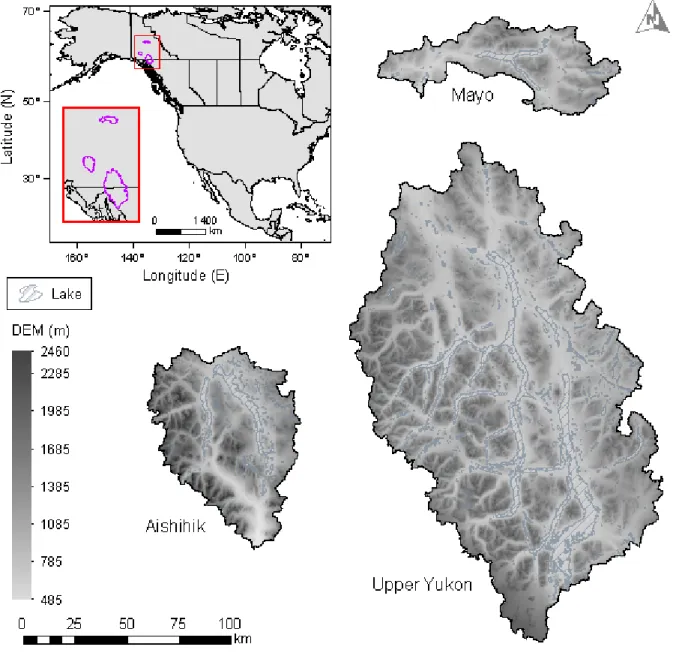
flow routing, and river flow routing, based on in situ discharge measurements, and (ii) snow states,
75
including snow depth, SWE, snowpack thermal deficit, snowpack liquid water content, and surface
76
albedo, based on snow survey data. The first DA routine was implemented by Samuel et al. (2019),
77
where the North American Ensemble Forecasting System (NAEFS) precipitation products are
78
merged into the operational flow forecasting platform in HYDROTEL through EnKF. The snow
DA routine, on the other hand, performs a distributed snow correction of the simulated snowpack
80
based on available in situ measurements. When snow surveys are available, the simulated state
81
variables including SWE and snow depth are corrected based on site measurements. The correction
82
is performed by interpolating the three nearest sites, where measurements are taken from, over the
83
entire watershed (Turcotte et al., 2007). Thus, the application of the snow DA routine in
84
HYDROTEL is in line with the same practice followed by a number of other forecasting centers
85
(see, e.g., Brasnett, 1999; Barrett, 2003; Drusch et al., 2004).
86
There are other sources of information, such as gridded numerical products, which can reduce
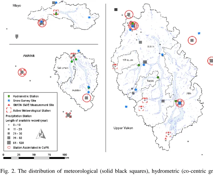
87
the input data uncertainty. For instance, the numerical weather prediction datasets produced by
88
Environment and Climate Change Canada (ECCC), which are adjusted through an assimilation
89
technique known as statistical interpolation (SI), represents a prime example of such atmospheric
90
analysis gridded precipitation products. Currently, these adjusted products are created by the
91
Canadian Precipitation Analysis (CaPA) system (Fortin et al., 2015; Mahfouf et al., 2007), the
92
product of which is known as the Regional Deterministic Precipitation Analysis (RDPA). The
93
CaPA-RDPA products are currently available in grib2 format on a polar-stereographic grid with a
94
10-km resolution (true at 60°N) at two temporal resolutions (6 hourly and 24 hourly). A
high-95
resolution version of the system, known as High Resolution Deterministic Precipitation Analysis
96
(CaPA-HRDPA) System is also in operation since 2018 and takes the HRDPS 2.5-km resolution
97
field as the trial.
98
The CaPA system has gained considerable momentum in recent years, and the suitability of
99
its precipitation products for application in hydrological modelling studies in Nordic watersheds
100
in Canada have been the subject of a number of studies (e.g., Deacu et al., 2012; Eum et al., 2014;
101
Gbambie et al., 2016; Haghnegahdar et al., 2014; Hanes et al., 2016; Wong et al., 2017; Zhao,
2013). Boluwade et al. (2018) compared the performance of CaPA-RDPA data against
103
precipitation observations in the Lake Winnipeg basin, which entails many of the
hydro-104
climatological characteristics associated with the northern Great Plains and concluded that
CaPA-105
RDPA data is a reliable precipitation product in sparsely gauged basin. Xu et al. (2019) evaluated
106
daily total precipitation data derived from CaPA-RDPA, ERA-Interim, ERA5, JRA-55,
107
MERRA-2, and NLDAS-2 over the Assiniboine River Basin, and concluded that in general, except
108
for convective rainfalls in summer, CaPA-RDPA products demonstrated the best performance
109
among all.
110
CaPA-RDPA data have also been used for establishing observational priorities in
poorly-111
instrumented basins in Canada. For instance, Abbasnezhadi et al. (2019) used the SI technique and
112
simulated the products and by-products of the CaPA system to design a stochastic meteorological
113
network density assessment scheme. In this approach, the network assessment is undertaken with
114
the objective to maximize the accuracy of precipitation products for hydrological modelling
115
applications. This scheme can be used to find the optimal density of a new observation network,
116
only if the RDPA products in the sparsely gauged region, where the observation network is
117
investigated for augmentation, are assumed to represent the truth. Given such a proposition, a
118
controlled assessment approach (one in which observation uncertainty is accounted for), as
119
suggested by Abbasnezhadi et al. (2019), would then be necessary to find the optimal station
120
density. However, the benchmark that the snow assimilation routine in HYDROTEL provides for
121
accurate flow estimation would mean that the accuracy of the CaPA-RDPA products could be first
122
validated prior to undertaking the network assessment. In other words, it is possible to claim or at
123
least expect that the current SWE correction performed in HYDROTEL can result in accurate
124
streamflow estimates against which the simulated streamflow for given CaPA-RDPA forcing can
be compared. Such an evaluation would provide us with valuable information (i.e., benchmark)
126
with respect to the accuracy or the intrinsic added-value of using the CaPA-RDPA products in
127
sparsely gauged basins for meteorological network assessment. Given this approach, it would then
128
be possible to perform the precipitation observation network assessment through a parsimonious
129
approach. Therefore, this study was designed to provide a framework for performing a
proxy-130
validation (i.e., indirect validation of gridded weather products by means of hydrological
131
modelling) of the RDPA products through the application of snow assimilation in physically-based
132
hydrologic models. The proxy-validation experiment and the network assessment framework
133
designed in this study can therefore be undertaken to complement the precipitation network
134
assessment approach designed by Abbasnezhadi et al. (2019). The assessment scheme introduced
135
in this study may also be implemented autonomously in sparsely gauged basins; providing that
136
snow survey data would be readily available.
137
The remainder of the paper is organized as follows. In Section 2, the study area is described
138
and specific details with respect to the hydrometeorological data used in the study are provided.
139
Section 3 describes the HYDROTEL model and outlines the approaches carried out to: (a) perform
140
HYDROTEL parameter sensitivity analysis and optimization, (b) validate the CaPA-RDPA
141
products through the application of the snow data assimilation routine in the model, and (c)
142
undertake the network assessment. Thereafter, results are presented and discussed in Section 4,
143
and conclusions are drawn in Section 5.
144
2. Study area and data characteristics
145
2.1 Study basins
146
Fig. 1 illustrates the location of the three study basins in Yukon, Canada, including the Mayo
147
River basin, Aishihik (/eyzhak/) River basin, and Upper Yukon River basin. These watersheds are
located in northern and mid-cordilleran alpine, sub-alpine, and boreal ecoclimatic regions (Strong,
149
2013) of central and southern Yukon. The Mayo basin covers a drainage area of roughly 2,670
150
km2. The mean annual precipitation and mean daily 2-m temperature are 456 mm (257 mm as rain;
151
199 mm as SWE) and −5.9°C, respectively (true for 1981-2018). The flow volume varies on a
152
seasonal basis, peaking in summer between June and July and dropping during winter in January
153
and December. There are two generating stations in Mayo: Mayo A and Mayo B. The Aishihik
154
basin covers a larger drainage area in the order of 4,550 km2 and is housing the Aishihik 155
hydroelectric Facility. The mean annual precipitation is around 302 mm (126 mm as rain; 176 mm
156
as SWE), and the mean daily annual 2-m temperature is in the order of –6.6°C (true for
1981-157
2018). The streamflow peaks in June, and the flow volume is relatively higher between May and
158
October (Brabets and Walvoord, 2009). The Upper Yukon River basin is the largest of the three
159
and covers a drainage area of around 19,600 km2. The basin is mountainous and is largely covered 160
by sporadic permafrost. Runoff in the Upper Yukon is derived primarily from snowmelt and
161
rainfall. The mean annual precipitation is around 299 mm (101 mm as rain; 198 mm as SWE), and
162
the mean daily annual 2-m temperature is in the order of –3°C (true for 1981-2018). The
163
streamflow peaks in August and is low between November and May. There is a generating station
164
in Whitehorse and one control structure on Marsh Lake. For all three basins, the dominant
165
hydrological processes are governed by snow accumulation and melting that produce high flow
166
volume which peaks in summer. In addition, the Upper Yukon River summer runoff involves
167
glacier melting from the southwest region of the basin.
168
-- Fig. 1 here --
2.2 Meteorological data
170
Table 1 provides a list of the meteorological stations located within and in the vicinity of the
171
boundaries of each basin. Except for MAYOMET and AISHMET stations, which are operated by
172
Yukon Energy (YE), the other stations are operated by the Meteorological Survey of Canada
173
(MSC).
174
-- Table 1 here --
175
Fig. 2 shows the distribution of the meteorological stations within and in the vicinity of the
176
study basins. In Mayo, the precipitation gauge at the Mayo airport (Mayo A), which is located just
177
in the outskirts of the basin, is the only historical active weather station with close to 100 years of
178
available record. The MAYOMET station located near the outlet of Mayo Lake was installed in
179
late 2018 and is the only active station within the basin. In Aishihik, the majority of the stations
180
(17 out of 27) have less than 25 years of available data. There are three active MSC stations within
181
a 75-km distance from the basin boundaries, including Carmacks CS (recording since 1999),
182
Haines Junction (recording since 1944), and the one at Burwash airport, which is 50 km east of
183
Aishihik, providing more than 50 years of historical precipitation data in conjunction with its
184
nearby stations (Burwash & Burwash A). Within the basin boundaries, however, there are only
185
two weather stations available (AISHMET & Otter falls NCPC), of which Otter falls NCPC has
186
not been recording since 2015, and AISHMET is the one which was activated in late 2018. In
187
Upper Yukon, more than 65% of the stations have less than 20 years of record, the majority of
188
which have been installed in the past 10 years. The MSC station at Atlin is the only historical
189
active station with more than 120 years of recorded precipitation amounts. It should be reminded
190
that solid precipitation undercatch is rather an important issue to consider when assimilating snow
191
measurements. Pierre et al. (2019) assessed the undercatch to be as much as 20-70% of the solid
precipitation, which is, to the authors’ knowledge, the most recent assessment available. This can
193
justify and explain why snow assimilation is necessary and beneficial.
194
-- Fig. 2 here --
195
The grib2 CaPA-RDPA v3.0.0 data from 2010 to 2018 at daily time steps were also
196
downloaded from ECCC ftp repository and decoded using NOAA/National Weather Service
197
wgrib2 program. The decoded data sets were then converted from the polar-stereographic grid onto
198
a rectangular grid covering each basin’s drainage area with a spatial resolution of 0.10° in latitude
199
and 0.15° in longitude (roughly 10 km in both directions at 60°N).
200
2.3 Hydrometric data
201
Table 2 provides a list of available hydrometric stations at which streamflow measurements
202
are taken in each basin (see Fig. 2 for the specific location of the hydrometric stations). The inflows
203
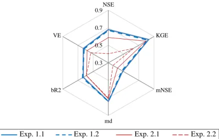
to Aishihik Lake and Mayo Lake do not represent naturally observed discharge values and were
204
reconstructed based on recorded water levels (see Samuel et al. (2019) for a detailed description
205
of the reconstruction methodology). For Mayo Lake, water level data obtained from the 09DC005
206
station and streamflow observed at the YECMAYO station were used for reconstructing inflows.
207
Similarly, water levels recorded at station 08AA005 and streamflow recorded at 08AA008,
208
08AA009, and 08AA010 stations were used to reconstruct the inflows to Aishihik Lake. All flows
209
and water levels were provided by the Water Survey of Canada (WSC), except for those at
210
reconstructed stations #0000003, ##0000003, and YECMAYO, which are recorded by YE.
211
Table 2 here
--212
2.4 Snow readings
213
Table 3 provides the metadata of the snow depth and SWE monitoring networks managed by
214
the Water Resources Branch (WRB) of Environment Yukon as well as the Gamma Monitoring
(GMON) automatic snowpack sensor readings provided by YE. The GMON (a.k.a. Campbell
216
Scientific CS725) sensor measures SWE by detecting the attenuation of naturally occurring
217
electromagnetic energy from the ground. This contactless approach can offer highly reliable and
218
accurate local SWE measurements with an uncertainty level that does not exceed ±5% at maximum
219
snow depth. Traditional SWE measurement approaches, such as the application of snow pillows,
220
by which the snowpack weight is directly measured, are prone to higher uncertainty levels since
221
snowpack properties (e.g., radiation characteristics) can be altered during the measurement. The
222
GMON gauge, which monitors snowpack properties in a contactless mode, does not suffer from
223
the same disadvantages. During the past few years, a number of GMON gauges were installed at
224
those locations identified in Table 3 and Fig. 2 (five stations were initially installed in Upper
225
Yukon, but two were removed and relocated; one in Mayo; and one in Aishihik). Once monitored,
226
the collected information is transmitted via satellite connection and goes through quality control.
227
Added and relocated GMON gauges intend to complete the existing snow survey site or at least
228
offer specific measurements within the basin limit (in Aishihik, Mayo). In situ snow measurements
229
are relevant and aim to capture snow evolution, but local measurements may not be representative
230
for the entire basin conditions.
231
-- Table 3 here --
232
3. Models and methodology
233
3.1 HYDROTEL: Sensitivity analysis and model calibration
234
The semi-distributed physically based HYDROTEL model can simulate a variety of
235
hydrological processes. These processes and the physically-based approaches used to simulate
236
each one along with a list of parameters associated with each process used in the version of
237
HYDROTEL utilized in this study are listed in Table 4. In HYDROTEL, the vertical water budget
is computed over a computational unit called the Relatively Homogeneous Hydrological Unit
239
(RHHU), which represents either a hillslope or elementary sub-watershed and are derived based
240
on a digital elevation model and a digital network of lakes and river sections using PHYSITEL, a
241
specialized GIS for distributed hydrological models (Turcotte et al., 2001; Rousseau et al., 2011;
242
Noël et al., 2014), both of which overlaid by a multi-layer soil model. The soil column of a RHHU
243
is stratified into three layers. The first soil layer (Z1) governs infiltration, and the other two layers
244
(Z2 and Z3) control interflow and baseflow. The interpolation of meteorological variables is based
245
on the weighted mean of the nearest three stations to resolve the amount of total precipitation,
246
which is then partitioned into rain and snow according to a threshold temperature and a simple
247
weighted scheme based on daily minimum and maximum temperatures, on each RHHU. For
248
missing station values, HYDROTEL fills the gap by using the values available at the three nearest
249
stations based on the inter-station temperature and precipitation altitude variations. The
250
accumulation and melt of snowpack processes are based on a mixed degree-day energy budget
251
approach and determine the timing and peak of the spring freshet. In the glacier module, a mixed
252
degree-day energy budget approach is also used in the exact same fashion used for the snowmelt
253
process. In the soil temperature and soil frost process, the only associated parameter (soil freezing
254
temperature threshold) is not distributed over the entire RHHUs, and therefore, is not
255
recommended to be modified. The next process is designed to identify the potential
256
evapotranspiration which is dominantly going to impact the total annual runoff and baseflow in
257
summer. The flow process at the RHHU scale simulates the water flux towards the river network
258
using a hydrogeomorphological unit hydrograph (a.k.a., HGM).
259
-- Table 4 here --
While other studies have performed different types of sensitivity analyses of HYDROTEL on
261
other basins (e.g., Bouda et al., 2013; Turcotte et al., 2003), a global sensitivity analysis was
262
performed using the Variogram Analysis of Response Surfaces (VARS) toolbox (Razavi et al.,
263
2019). The toolbox allows the user to identify the parameters by the importance level (i.e., model
264
sensitivity to changing parameter conditions) through a multi-method approach that unifies
265
different theories and strategies. With sensitive parameters in hand, the model calibration becomes
266
a less challenging task. However, since calibration of HYDROTEL, in essence, is a multi-objective
267
optimization problem (due to the number of stream gauges reporting flows in the basin for which
268
several error criteria might be assessed), defining what makes the model calibrated is not a
269
straightforward task. Moreover, other factors affecting the quality of the calibration result include
270
error due to lake/reservoir inflow reconstruction and the quality of precipitation or temperature
271
forcing data (elaborating on these concerns is beyond the scope of the current study). To properly
272
respond to these challenges, model calibration was completed in OSTRICH (Optimization
273
Software Toolkit for Research Involving Computational Heuristics), which is a
model-274
independent and multi-algorithm optimization tool (Matott, 2017). The toolkit, which supports
275
both single- and multi-criteria optimization options, can be used for the weighted non-linear
least-276
squares calibration of the model parameters or for constrained optimization of a set of design
277
variables according to pre-defined cost functions. OSTRICH can incorporate different algorithms
278
to search for the optimal value of the objective functions and to identify the set of parameter values
279
associated with such optima. There are several optimization algorithms available in the toolkit,
280
which can be classified as either deterministic local or heuristic global search methods
281
incorporating elements of structured randomness. For multi-criteria optimization, the Pareto
282
Archive Dynamically Dimensioned Search (PA-DDS; Asadzadeh and Tolson, 2009, 2013) and the
simple multi-objective optimization heuristic algorithms are available, while for uncertainty-based
284
calibration, several sampling-based algorithms (i.e., Generalized Likelihood Uncertainty
285
Estimation and Metropolis-Hastings Markov Chain Monte Carlo) are available. In addition, the
286
asynchronous parallel processing architecture provided by OSTRICH, which is based on the
287
industry standard Message Passing Interface (MPI), provided the means to speed up the calibration
288
procedure.
289
The model was calibrated for the period of 2010-2018 using PA-DDS by maximizing the
290
Kling-Gupta Efficiency (KGE; Gupta et al., 2009) and minimizing the root mean squared errors
291
(RMSE). HYDROTEL was forced with CaPA-RDPA and meteorological data, including daily
292
precipitation and maximum and minimum temperatures time series described in Table 1, as well
293
as snow survey observations provided in Table 3. Daily historical discharge data measured at the
294
location of available hydrometric stations described in Table 2 and identified in Fig. 2 were
295
obtained from WSC, while the reconstructed inflows were calculated and used for model
296
calibration.
297
3.2 Impact of snow data assimilation and CaPA-RDPA forcing
298
In order to investigate the impact of SWE assimilation on model performance, and also to
299
understand how robust the accuracy of CaPA-RDPA products were over the three study basins for
300
hydrologic application purposes, two separate sets of modelling experiments were designed. In the
301
first set (experiment Set 1), the model was trained with forcing CaPA-RDPA, while in the second
302
set (experiment Set 2), MSC meteorological data were used as input. Depending on whether the
303
GMON and snow survey monitoring information were assimilated during the calibration and the
304
‘stand-alone’ run (i.e., when the model runs once the calibration is completed), two separate runs
305
were considered for each set (see Table 5). In Exp. 1.1, the model was calibrated while assimilating
SWE measurements. The assimilation was then switched off and the calibrated model was forced
307
with CaPA-RDPA once again for the same time period (2010-2018) (Exp. 1.2). This experiment
308
was designed to indicate the extent by which the model would be able to preserve the flow
309
estimation accuracy with forcing precipitation analysis products only. The second set of
310
experiments (Exp. 2.1 and Exp. 2.2) are similar to those in the first set except that CaPA-RDPA
311
data were replaced with gauged meteorological forcing. For each experiment, goodness-of-fit
312
metrics can be used to quantitatively measure the representativeness of the experimental flow
313
estimations to the hydrometric observations (the metrics used in this study can be found in the
314
supplementary materials provided in the online version of this paper). Such an evaluation helped
315
us perform an inter-comparison of the results between the two sets of experiments.
316
-- Table 5 here --
317
3.3 Network assessment
318
Depending on whether the former assessment of the CaPA-RDPA forcing in HYDROTEL
319
may suggest if the gridded analysis products can be adequately used for streamflow simulation, a
320
simple network density sensitivity analysis based on CaPA gridded products was proposed for
321
flow simulation in HYDROTEL. Such an assessment was designed to guide future network
322
assessment procedures. Therefore, a network assessment procedure similar to that of
323
Abbasnezhadi et al. (2019) was followed here, except that the assessment did not include
324
artificially generated reference fields. Rather, a subset of grid points was extracted to create
325
network scenarios of different resolutions from the RDPA domain over each basin, while the
326
respective precipitation analysis was directly used during the assessment. Such an uncontrolled
327
framework could be specifically useful for the case of this study as the SWE DA-CaPA coupling
328
could prove to output such streamflow estimation that could closely match flow observations.
Sampling grids (Θ𝜈), where 𝜈 is the resolution of the pseudo-network in decimal arc-degrees, 330
pertaining to each study basin are defined in Table 6 (refer to the supplementary materials to see
331
individual scenarios for each basin).
332
-- Table 6 here --
333
4. Results and Discussion
334
4.1 Sensitivity analysis and model calibration
335
The results of the sensitivity analysis provided by VARS indicated that among the parameters
336
used to regulate the vertical water budget, the second soil layer thickness (Z2), which affects flow
337
peaks, is a sensitive parameter. The third soil layer thickness (Z3), which mostly affects baseflow,
338
was identified to be a less sensitive parameter in this group. Also, the recession coefficient (CR),
339
which affects summer baseflow and works with Z3, was found to be a relatively sensitive
340
parameter. Among the parameters used for calculating the weighted mean of the nearest three
341
stations, VARS indicated that the third parameter in this group (PPN) has more impact on the
342
results, and the first two (GT and GP) are almost equal in sensitivity. Also, for the snow processes,
343
the melting temperature thresholds and rates for all three land classes in this group (SFC, SFF,
344
SFD, TFC, TFF, TFD) were shown to have equal sensitivity levels. Both glacier melting
345
parameters (MR and TT) were found to be sensitive too, and the multiplicative coefficient (FETP)
346
applied to the Penman-Monteith equation was found to be the only sensitive evapotranspiration
347
parameter. None of the parameters related to the flow process at the RHHU scale was found to be
348
sensitive, while any modification to these parameters would force the model to recalculate the
349
HGM file which would be time-consuming. The parameters associated with the channel flow
350
process, computed using the kinematic wave equation, were also not found to be sensitive.
Previous VARS applications performed by Foulon et al. (2019) in two basins in southern
352
Québec yielded different results for the vertical water budget parameters. Z1 was shown to be the
353
least sensitive soil layer thickness, while Z2 and Z3 were the second most and the most sensitive
354
parameters, respectively. Also, the recession coefficient (CR) was indicated to be one of the most
355
sensitive parameters in the model. This signifies that HYDROTEL is rather sensitive to basin
356
location and governing hydrological processes. In fact, Yukon and southern Québec are both
357
governed by snow accumulation and melt, yet summer baseflow plays a more prominent role in
358
southern Québec.
359
With sensitive parameters in hand, comprising of a set of 16 parameters indicated in Table 4
360
by those with the importance level of 1, the model was calibrated in OSTRICH. The standard upper
361
and lower bound values used for each parameter in OSTRICH are provided in Table 4, which are
362
based on the physical meaning of each parameter and the works of Fortin et al. (2001b) and
363
Turcotte et al. (2003). Also, the initial estimates for each parameter were based on those derived
364
in previous calibration efforts, in which each parameter was manually adjusted in order to achieve
365
the desired hydrological performance. The toolbox utilized eight computational cores for
366
asynchronous parallel processing at the budget of 2-18 hours (depending on the basin’s drainage
367
area) for 1000 iterations.
368
In Mayo, the model calibration was completed in OSTRICH based on the inflow time-series
369
into Mayo Lake associated to YE gauge ##0000003 (see Fig. 2). In Aishihik, the model calibration
370
was completed in two stages. In the first stage, the model was calibrated for Sekulmun River
371
streamflow time-series at the outlet of Sekulmun Lake observed at WSC Gauge 08AA008 (see
372
Fig. 2). The Sekulmun portion of the Aishihik model was isolated and separated in HYDROTEL
373
GUI (graphical user interface) to decrease the model run time. In the second stage, the model was
setup to simulate the reconstructed inflow time series to Aishihik Lake associated with YE gauge
375
#0000003. The original reconstructed inflow data display high-intensity fluctuations and were not
376
deemed suitable for the calibration. Instead, they were first smoothed by using a 7-day moving
377
average window (windows of longer durations were also tested and did not show to enhance the
378
calibration results). In Upper Yukon, the model calibration was also performed in two stages. In
379
the first stage, the model was calibrated separately for three gauged sub-basins, including Atlin
380
River (WSC gauge 09AA006), Tutshi River (WSC gauge 09AA013), and Wheaton River (WSC
381
gauge 09AA012) (see Fig. 2). In the second stage, the model was then setup to simulate the flow
382
time series in Yukon River at Whitehorse observed at WSC gauge 09AB001.
383
Fig. 3 shows the flow duration curves for Mayo, Aishihik (including the Sekulmun sub-basin),
384
and Upper Yukon (including the Atlin, Tutshi, and Wheaton sub-basins) (refer to the
385
supplementary materials provided in the online version of this paper to see discharge time-series).
386
In Mayo, the simulation has fully preserved the exceedance probability of observed flows. In
387
Aishihik and Sekulmun, other than some overestimation of winter low flows, the remainder has
388
been well captured by the model. In Upper Yukon, in general, the exceedance probabilities of the
389
simulated flows closely resemble the observed ones although the low flows are underestimated in
390
sub-basins with small drainage areas (Tutshi and Wheaton), which has similarly impacted the low
391
flows in Yukon too. In Atlin, the exceedance probability of the observed high flows (corresponding
392
to the flow peaks) is marginally underestimated.
393
-- Fig. 3 here --
394
4.2 Proxy validation of CaPA-RDPA
395
The impact of the snow DA routine in HYDROTEL and CaPA-RDPA forcing data on
396
modelling results were assessed based on the set of experiments discussed in Section 3.2. Fig. 4
compares the metrics in Mayo for the first and the second sets of experiments (for the full
398
description of the metrics used in the figures of this section, see the supplementary materials in the
399
online version of this paper). The metrics reported by the experiments indicate that the calibration
400
results for the case when CaPA-RDPA are used as input (Exp. 1.1 and Exp. 1.2) surpass, in both
401
cases, those derived by station observations (Exp. 2.1 and Exp. 2.2). In addition, the best outcome
402
is obtained with Exp. 1.1 when the model calibration is performed with CaPA-RDPA forcing and
403
the snow DA routine in active mode. Exp. 1.2 (CaPA-RDPA forcing and no snow DA), on the
404
other hand, indicates that the model’s performance is not undermined if the snow DA routine is
405
turned off in HYDROTEL (when the model has already been calibrated with the snow DA routine
406
in active mode). In other words, for this experiment, the assimilation of snow monitoring data has
407
relatively no impact on the flow estimation accuracy if CaPA-RDPA data are used as input. In
408
contrast, the metrics obtained from the second set of experiments indicate that when the model is
409
calibrated using MSC meteorological data as input and with the snow DA routine in active mode
410
(Exp. 2.1), the metrics are on the ballpark of an acceptable level, while still falling short of those
411
obtained with CaPA-RDPA. However, as Exp. 2.2 indicates, if the snow DA routine is turned off,
412
the flow estimation accuracy declines significantly. This illustrates that for the second set of
413
experiments with sparsely gauged meteorological input data, the snow DA routine has a
414
compensating impact on the flow estimation accuracy.
415
Although the new GMON stations do not provide a long record of measurements yet, the snow
416
course sites in all three basins provide long-enough and continuous records of snow depth and
417
SWE measurements. Results from the second set of experiments shown in Fig. 4 indicate that, in
418
Mayo, these snow course measurements provide valuable information by which the SWE data
419
simulated using the meteorological network can be corrected through the snow assimilation routine
in HYDROTEL. In other words, the flow estimation accuracy in Mayo is highly dependent on the
421
external information from the snow survey sites. Although this outcome does not indicate the
422
representativeness of the snow survey sites, it hints at their value. The same debate is found in the
423
literature where hydrological models, for example, are run by interpolating snow depth
424
measurements from a few selected sites to larger areas despite their limited spatial
425
representativeness (Grünewald and Lehning, 2015; López-Moreno et al., 2013). Other studies have
426
quantified the issue of snow sites representativeness. For example, Winstral and Marks (2014)
427
proved that an index site representative of the basin conditions can be valid for a basin wide SWE
428
in most years.
429
On the other hand, the proxy validation of the CaPA-RDPA in Mayo based on the
430
reconstructed inflow associated with gauge ##0000003 shows that the analysis is accurate enough
431
to the extent that would not call for any correction through snow measurements. To this point,
432
these results indicate that in Mayo: (a) CaPA-RDPA products can be used for flow estimation, (b)
433
given the fact that very few precipitation stations are currently assimilated in CaPA, if the current
434
network is extended, the modelling accuracy will improve, and (c) in the absence of a precipitation
435
observation network with an optimal density, the snow assimilation routine plays a significant role
436
to compensate for proper precipitation information.
437
-- Fig. 4 here --
438
Fig. 5a compares the metrics in Aishihik for the first and the second sets of experiments, while
439
the performance of the model in response to the set of experiments completed in Sekulmun are
440
shown in Fig. 5b. The results reported for both Aishihik and Sekulmun are not identical to those
441
of Mayo and the experiments rather exhibit a contrasting outcome. While in Mayo, deactivating
442
the snow assimilation routine in HYDROTEL when forcing the model with CaPA-RDPA
(Exp. 1.2) would marginally impact the metrics compared to the case when the snow assimilation
444
routine was active (Exp. 1.1), in Aishihik (including the Sekulmun sub-basin), deactivating the
445
snow assimilation routine led the model performance to decay significantly. This suggests that the
446
RDPA gridded products do not encompass the required accuracy over Aishihik, rendering the
447
assimilation of snow readings an essential component for accurate flow estimation. The
448
inadequacy of the RDPA estimates over Aishihik is an indication of the detrimental impact of the
449
sparse precipitation network in Aishihik, which encompass a relatively larger drainage area, on
450
CaPA products over the basin. In Sekulmun, Exp. 2.2 provides marginally better results than Exp.
451
2.1, demonstrating that the precipitation measurements taken at the MSC meteorological stations
452
better represent the ground SWE accumulation than those recorded at the snow course sites.
453
Nevertheless, in Sekulmun, when using CaPA-RDPA data as the input, the combined effect of
454
incorporating the value of information from both the external assimilation of precipitation data in
455
CaPA and the internal assimilation of snow readings in HYDROTEL has obviously improved the
456
flow estimation accuracy (see Fig. 5b). In Aishihik, however, Exp. 2.1 displays a declined
457
performance relative to Exp. 1.1, while Exp. 2.1 and Exp. 2.2 are relatively identical. These results,
458
in total, revealed that in Aishihik and Sekulmun, the snow data are essential for accurate flow
459
estimation if the model is forced with CaPA-RDPA, while the MSC precipitation input data seems
460
to deliver sufficient accuracy (indicating the accuracy of the precipitation measurements taken as
461
MSC stations which necessitates minimal correction by the data taken at the snow course sites).
462
This, once again, indicates that the value of precipitation information from the MSC precipitation
463
gauges is superior to those of CaPA-RDPA which illustrates the low accuracy of CaPA data over
464
the basin.
465
-- Fig. 5 here --
Fig. 6 compares the metrics in Upper Yukon, including those for Atlin, Tutshi, and Wheaton
467
for the first and the second sets of experiments. In Atlin (Fig. 6a), there are marginal differences
468
between the results derived from all four experiments. This agreement could be the outcome of
469
several factors, including: (a) co-location of the snow course site and the MSC gauge in Atlin, (b)
470
existence of a MSC gauge which is assimilated in CaPA (see Fig. 2); forcing the respective RDPA
471
over the basin to become more or less identical to that of gauge reading, (c) the impact of the
472
nearby MSC gauges on the northeast side of the basin (just beyond the basin boundary) on the
473
accuracy of precipitation estimate over the basin. In Tutshi and Wheaton, however, a different
474
outcome is evident. The impact of drainage area on the flow estimation accuracy for the given
475
activity state of the snow assimilation routine seems to be a factor of importance. For instance, for
476
a sub-basin such as Tutshi (Fig. 6b) with a small drainage area, the impact of the only snow course
477
site in the basin (site #09AA-SC3) on the flow accuracy can be comprehended by the fact that
478
deactivating the snow assimilation in Exp. 2.2 has significantly decayed the flow accuracy by
479
almost half. On the other hand, in Wheaton (Fig. 6c), a sub-basin with a comparable drainage area
480
to that of Tutshi, in the absence of any snow course site, Exp. 2.2 has apparently yielded about the
481
same metrics obtained from Exp. 2.1. In general, the results of the experiments performed in Upper
482
Yukon indicate that since the basin generally enjoys a higher number of weather stations (including
483
those assimilated in CaPA and snow course sites), the results demonstrate better metric values.
484
-- Fig. 6 here --
485
Table 7 summarizes the significance of the snow assimilation routine for each basin for the
486
given meteorological forcing. In short, activating the snow assimilation routine would have a
487
significant impact on the flow estimation only in Mayo when forcing HYDROTEL with the MSC
488
meteorology and in Aishihik when forcing the model with CaPA-RDPA data. Hence, it appears
that snow survey sites are more representative of the watershed snow conditions than the
490
meteorological conditions recorded at the MSC stations or embedded into CaPA-RDPA.
491
In Upper Yukon, sub-basins did not yield consistent results. It was shown that the model does
492
not necessarily need the assimilation of snow products when the model is forced with either gauged
493
or analysis precipitation products (for 3 out of 4 sub regions). While medium-size watersheds (as
494
Tutshi) could benefit from snow survey measurements, the others could not. For larger watershed
495
with denser meteorological networks, snow assimilation may prove to be superfluous. Overall,
496
where snow assimilation significantly improves the results, it can be concluded that the
497
corresponding meteorological forcing does not have the expected accuracy for hydrologic
498
modelling purposes, including the assessment of the meteorological network density which is the
499
subject of the next analysis in this study.
500
-- Table 7 here --
501
4.3 Network sensitivity analysis
502
The information gained from the validation stage was used to decide whether the assessments
503
should be undertaken with/without the assimilation of snow course data. The proxy validations
504
indicated that at least in Aishihik, CaPA data do not have the required accuracy, while the
505
validations in the other two basins (Mayo and Upper Yukon) were promising. Therefore, in
506
Aishihik, the network assessment was carried out while assimilating the snow course
507
measurements. In Mayo and Upper Yukon, no snow assimilation was performed when evaluating
508
the impact of different network scenarios. Even though any proposed additional station would
509
probably be equipped with various measuring apparatus for different meteorological variables, the
510
network augmentation assessment was carried out with the assumption that the network would be
mainly measuring precipitation. This is mainly due to the fact that precipitation demonstrates a lot
512
more spatial variability than other meteorological variables (e.g., temperature, wind).
513
Fig. 7 shows the variation of the NSE, KGE, and absolute PBias scores in Mayo, Aishihik,
514
and Upper Yukon with the changing resolution of the pseudo-network scenarios (for descriptions
515
of the scores, see the supplementary materials). In Mayo (thick lines in all figures), as the network
516
resolution decreases (and so does the network density) from 0.10° to 0.35°, the scores go through
517
two distinct areas of variation. First, decreasing the network resolution from 0.10° to 0.30° results
518
only in marginal drops in all three performance scores. In comparison, the performance of the
519
CaPA precipitation products for a network with a given resolution of 0.30° or higher is better than
520
that of the current meteorological precipitation network (shown by horizontal lines). The
521
fluctuations and the unexpected drops in performance scores in this range are an artifact of the
522
spatial variability of precipitation that has not been fully resolved by certain grid points. This
523
phenomenon which is known as singularity has been reported previously by Abbasnezhadi et al.
524
(2019) and Dong et al. (2005). Decreasing the network density below 0.30°, results in substantial
525
performance deterioration to an extent well below the current sparse MSC network. This indicates
526
that the limit at which the CaPA gridded data can outperform the existing network in Mayo is
527
limited to a network with a density of at least 0.30°.
528
-- Fig. 7 here --
529
The variation of the NSE, KGE, and absolute PBias in Aishihik with changing network
530
resolution are shown by dashed lines and compares the performance of the pseudo-network
531
scenarios constructed based on the CaPA grid definition with the current MSC network in the
532
basin. The same overall trend of variation previously observed in Mayo is evident here too where
533
the scores drop (although less abruptly) after negligible changes before the threshold network
density. The less sudden drop is an expected attenuation consequence of a larger drainage area
535
which is more evidently manifested by the NSE scores which is known to be a sensitive parameter
536
to peak discharge values (see Abbasnezhadi et al., 2019 for the same performance outcome). In
537
Aishihik, the network resolution threshold cannot be explicitly inferred. The variation of the NSE
538
indicates that for every decrease in resolution there is a decrease in performance that is rather of
539
the same order of magnitude for all resolutions, whereas those of KGE and PBias assert the 0.4°
540
pseudo-network to entail the optimal resolution below which the accuracy of the ensued flow
541
simulations degrades significantly. Any higher-density network would cause the scores to level
542
off and little would be gained by further increasing the network density. The asserted network
543
density threshold of 0.4° derived for Aishihik resembles the performance established by the current
544
MSC meteorological network in the basin. Moreover, this threshold value is also slightly higher
545
than the one determined for Mayo. This was an anticipated outcome as in basins with a larger
546
drainage area, representativeness errors are averaged out which makes missing a storm event less
547
impactful on the overall network precision. In contrast, in smaller basins (as in Mayo), mesoscale
548
precipitation systems are essentially significant for capturing proper flow statistics. Accordingly,
549
a higher network threshold value can already be anticipated for Upper Yukon which has an even
550
larger drainage area than that of Aishihik.
551
In Upper Yukon (thin lines), the same features previously observed in Mayo and Aishihik are
552
apparent, while a higher network threshold value is resolved. Similar to what was indicated for
553
Aishihik, a network resolution threshold cannot be explicitly inferred in Upper Yukon. Arguably,
554
if Pbias changes are ignored (which asserts the 0.7° pseudo-network to entail the optimal
555
resolution), it can be claimed that the 0.5° pseudo-network would be optimal. A pseudo-network
556
with a density threshold value between 0.5° and 0.7° would as such provide an optimal resolution
range. Quite interestingly, the current MSC network maintains an accuracy which is comparable
558
in performance to the highest network density of the original CaPA network.
559
5. Summary and Conclusions
560
This study is at the crossroad between meteorological data assimilation (in which precipitation
561
observations are merged into numerically modelled precipitation data), and hydrological data
562
assimilation (in which snow survey data are merged into streamflow forecast). Before applying
563
assimilated precipitation products in meteorological network assessment, first it is required to
564
validate the accuracy of these products. In this study, it is indicated that since assimilation of snow
565
survey data could provide the benchmark for accurate flow estimation, it would then be possible
566
to evaluate the accuracy of precipitation assimilation products through the proxy-validation of
567
precipitation analysis in such a hydrologic system. The HYDROTEL model snow data assimilation
568
(DA) routine is one such example which provides the opportunity to investigate the added value
569
of using the CaPA-RDPA data for application in meteorological network assessment in sparsely
570
gauged Nordic basins.
571
The hydrologic footprint of CaPA-RDPA data and MSC ground observations were validated
572
against hydrometric observations. This validation was performed to examine whether assimilating
573
snow monitoring information in HYDROTEL can offset the adverse effects of precipitation data
574
scarcity in Yukon. When snow assimilation could significantly improve the flow simulation
575
outcomes, it was concluded that the corresponding meteorological forcing (either CaPA-RDPA
576
data or ground observations; in this instance, MSC stations) could not exclusively provide the
577
required accuracy for hydrologic modelling purposes. The proxy validation of the CaPA-RDPA
578
data indicated that the gridded analysis products enjoy the level of accuracy required for accurate
579
flow simulation in Mayo and Upper Yukon which does not entail the application of snow
assimilation in HYDROTEL. In Aishihik, however, the validations demonstrated that the regional
581
precipitation analysis does not have the required accuracy, and therefore, assimilation of observed
582
snow course information had a significant impact on the flow estimation accuracy. Based on the
583
results of these experiments, it can be concluded that although these basins are all located within
584
similar ecoclimatic zones in southern Yukon and in the proximity of each other, the distribution
585
of snow course sites and precipitation gauges have left a substantial impact on the accuracy of
586
precipitation and snow assimilation procedures which directly affect the accuracy of flow
587
simulations. These results indicate the importance of the snow assimilation routine in HYDROTEL
588
to embed crucial information not readily available from precipitation forcing data. This approach
589
and the lessons learned may also benefit watersheds in other parts of the world facing similar
590
challenges related to incorporating accurate data when such information is not embedded within
591
the forcing data.
592
With the experiments in hand, a network augmentation assessment was carried out
593
subsequently by incorporating the value of data and products available from the CaPA assimilation
594
system with the assumption that the network would be mainly measuring precipitation. The
595
assessment indicated that a number of additional stations can be installed in each basin to increase
596
the accuracy for streamflow simulation. It is worth reiterating that the analysis was performed
597
based on CaPA-RDPA data and having real measurements on the ground could prove to require
598
fewer stations, especially for Aishihik and Mayo. In addition, the network was assessed in an
599
uncontrolled mode where no observation error was added during the analysis to simulate the
600
impact of such errors (including those related to solid precipitation in winter and convective storms
601
during summer). Instead, CaPA-RDPA data were used directly into the assessment since the
602
assumption of accuracy was validated prior to undertaking the assessment. Given that in the CaPA
system, precipitation measurements are subjected to various quality control (QC) procedures
604
before being assimilated, the RDPA products can, therefore, be assumed to be of relatively proper
605
quality. However, the implication of such an assumption is that, the optimal number of stations
606
derived for each basin is valid when those stations satisfy CaPA QC procedures too. In other words,
607
if the quality of measurements available from the proposed extended network can satisfy CaPA
608
QC, they could equally benefit the CaPA system. Moreover, it is ultimately beneficial if any
609
additional precipitation station which can be directly used for flow forecasting in HYDROTEL
610
may also be used for the similar purpose indirectly when embedded into the products of the CaPA
611
assimilation system. Also, if existing snow survey sites could provide the required SWE data for
612
hydrologic snow assimilation, the framework introduced in this study could be easily
613
implemented. Otherwise, in case a network assessment is to be undertaken in a basin where such
614
data are not readily available, proper arrangements should be made to first conduct snow surveys.
Acknowledgements
616
The authors wish to gratefully acknowledge the financial support from Natural Sciences and
617
Engineering Research Council of Canada (NSERC) and Yukon Energy (YE) through
618
Collaborative (#CRDPJ 499954-16) and Applied (#CARD2 500263-16) Research and
619
Development grants. This project would not have been possible without substantial contributions
620
from staffs at Yukon Research Centre, namely Brian Horton and Maciej Stetkiewicz; at INRS,
621
Sébastien Tremblay; and at YE, Shannon Mallory, Kevin Maxwell, and Andrew Hall. We would
622
like to also acknowledge the following organizationsfor their readily available online data used in
623
this study: Meteorological Survey of Canada, Water Survey of Canada, Environment and Climate
624
Change Canada, Water Resources Branch at Environment Yukon, Yukon Energy, and Natural
625
Resources Conservation Service at United States Department of Agriculture. The authors declare
626
no conflict of interests in this work.
References
628
Abbasnezhadi, K. 2017. Influence of meteorological network density on hydrological modeling
629
using input from the Canadian Precipitation Analysis (CaPA). PhD Thesis, Winnipeg, 630
Manitoba, Canada: University of Manitoba. http://hdl.handle.net/1993/32177.
631
Abbasnezhadi, K., A. N. Rousseau, K. A. Koenig, Z. Zahmatkesh, and A. M. Wruth. 2019.
632
"Hydrological assessment of meteorological network density through dataassimilation
633
simulation." Journal of Hydrology 569: 844-858.
634
doi:https://doi.org/10.1016/j.jhydrol.2018.12.027.
635
Andreadis, K. M., and D. P. Lettenmaier. 2006. "Assimilating remotely sensed snow
636
observations into a macroscale hydrology model." Advances in Water Resources 29:
872-637
886. doi:https://doi.org/10.1016/j.advwatres.2005.08.004.
638
Arulampalam, M. S., S. Maskell, N. Gordon, and T. Clapp. 2002. "A tutorial on particle filters
639
for on-line nonlinear/non-Gausssian Bayesin tracking." IEEE Transactions on Signal
640
Processing 50: 174-188. doi:https://doi.org/10.1109/78.978374. 641
Asadzadeh, M., and B. Tolson. 2009. "A New Multi‐ objective Algorithm, Pareto Archived
642
DDS." Edited by G. et al. Raidl. 11th Annual Conference on Genetic and Evolutionary
643
Computation Conference (GECCO 2009). New York, NY: Association for Computing 644
Machinery. 1963-1966. doi:https://doi.org/10.1145/1570256.1570259.
645
Asadzadeh, M., and B. Tolson. 2013. "Pareto archived dynamically dimensioned search with
646
hypervolume-based selection for multi-objective optimization." Engineering Optimization 45
647
(12): 1489-1509. doi:https://doi.org/10.1080/0305215X.2012.748046.
648
Barrett, A. P. 2003. National operational hydrologic remote sensing center snow data
649
assimilation system (SNODAS) products at NSIDC. Special Rep. 11, Boulder, CO, USA: 650
NSIDC, 19. Accessed December 14, 2018.
651
https://nsidc.org/pubs/documents/special/nsidc_special_report_11.pdf.
652
Boluwade, A., K.-Y. Zhao, T. Stadnyk, and P. Rasmussen. 2018. "Towards validation of the
653
Canadian Precipitation Analysis (CaPA) for hydrologic modeling applications in the
654
Canadian Prairies." Journal of Hydrology 556: 1244-1255.
655
doi:https://doi.org/10.1016/j.jhydrol.2017.05.059.
656
Boni, G., F. Castelli, S. Gabellani, G. Machiavello, and R. Rudari. 2010. "Assimilation of
657
MODIS snow cover and real time snow depth point data in a snow dynamic model."
658
Geoscience and Remote Sensing Symposium (Geoscience and Remote Sensing Symposium) 659
1788-1791. doi:https://doi.org/10.1109/IGARSS.2010.5648989.
660
Bouda, M., A. N. Rousseau, B. Konan, P. Gagnon, and S. J. Gumiere. 2012. "Bayesian
661
Uncertainty Analysis of the Distributed Hydrological Model HYDROTEL." Journal of
662
Hydrologic Engineering 17 (9): 1021-1032. doi:https://doi.org/10.1061/(ASCE)HE.1943-663
5584.0000550.