HAL Id: pastel-00005945
https://pastel.archives-ouvertes.fr/pastel-00005945
Submitted on 21 Jul 2010
HAL is a multi-disciplinary open access archive for the deposit and dissemination of sci-entific research documents, whether they are pub-lished or not. The documents may come from teaching and research institutions in France or abroad, or from public or private research centers.
L’archive ouverte pluridisciplinaire HAL, est destinée au dépôt et à la diffusion de documents scientifiques de niveau recherche, publiés ou non, émanant des établissements d’enseignement et de recherche français ou étrangers, des laboratoires publics ou privés.
dans les semi-conducteurs
Thi Lam Hoai Nguyen
To cite this version:
Thi Lam Hoai Nguyen. Propriétés de spin des états évanescents et effet tunnel dans les semi-conducteurs. Physique [physics]. Ecole Polytechnique X, 2010. Français. �pastel-00005945�
THÈSE
Présentée pour obtenir
Le GRADE de DOCTEUR de l’ÉCOLE POLYTECHNIQUE
Discipline : PHYSIQUE par
Nguybeen Thi. Lbam Hoai
PROPRIÉTÉS DE SPIN DES ÉTATS ÉVANESCENTS ET
EFFET TUNNEL DANS LES SEMI-CONDUCTEURS
SPIN PROPERTIES OF EVANESCENT STATES AND
TUNNELING IN SEMICONDUCTORS
Soutenue le 21 janvier 2010 devant la commission d’examen:
Xavier MARIE Président
Robson FERREIRA Rapporteur
Henri JAFFRES Rapporteur
Joël CIBERT Examinateur
Henri-Jean DROUHIN Directeur de thèse
Guy FISHMAN Co-Directeur de thèse
Thèse préparée au Laboratoire LSI de l’École Polytechnique et au Laboratoire IEF de l’Université Paris 11
J’aimerais tout d’abord exprimer mon infinie reconnaissance à mes deux directeurs de thèse — MM. Henri-Jean Drouhin et Guy Fishman — qui se sont toujours occupés de moi dès le premier jour de mon arrivée en France et sans les-quels cette thèse n’aurait pu se réaliser. Je vous remercie beaucoup, Henri-Jean et Guy, pour m’avoir introduite à la vie scientifique. Merci pour vos explications sur les « subtilités », sur les « sous-entendus » de la physique qui ont, sans aucun doute, clarifié mes pensées parfois naïves et embrouillées. Merci pour votre pré-sence attentive et soutenue pour répondre à toutes mes questions, qu’elles aient été petites ou grandes, difficiles ou évidentes, bonnes ou erronées. Merci pour les idées directrices de la thèse, les discussions instructives entre nous, la vision sur la signification des résultats obtenus : ce sont des ressources précieuses de la thèse. Merci de n’avoir jamais perdu confiance en moi, de m’avoir prodigué des encouragements pour chaque petite « victoire » et de m’avoir encouragée aux moments les plus difficiles où on s’est aperçu des erreurs et retrouvé au point de départ. Mes mots ne peuvent exprimer toute ma gratitude, mes remerciements. Je suis très heureuse d’avoir eu la chance de vous connaître et de travailler avec vous. Je tiens aussi à remercier MM. Robson Ferreira et Henri Jaffres qui ont accepté d’évaluer mon travail. Je remercie également M. Joël Cibert d’avoir fait partie du jury. Je remercie vivement M. le Professeur Xavier Marie qui m’a fait l’honneur de présider le Jury. Je remercie l’ensemble du jury pour ses questions pertinentes qui m’ont permis d’appréhender le sujet en profondeur.
Je remercie les équipes du Laboratoire des Solides Irradiées, Ecole Poly-technique et de l’Institut de Physique Fondamentale de l’Université Paris-Sud de m’avoir accueillie dans leurs lieux respectifs.
Je remercie en particulier Travis Wade pour les corrections de l’anglais concernant les articles et pour le manuscrit.
Je remercie Juliette Mangeney et ses deux doctorants Loïc Meignien et Matthieu Martin pour la grande gentillesse dont ils ont fait preuve avec leur
co-Je remercie Thi-Phuong Ngo, Viet-Hung Nguyen, Eloy Ramirez-Garcia, Quang-Anh Nguyen, Mihaela-Cristina Ciornei, Feng Yang - mes amis à IEF et au LSI - pour les petits moments où on faisait une pause et parlait de notre tra-vail. Grand merci à tous mes amis de l’X avec qui j’ai partagé la vie quotidienne pendant plus de trois années sur le « Plateau venteux » et qui m’ont beaucoup aidée à surmonter les moments difficiles.
Je remercie tous ceux et celles qui, malgré la distance et l’éloignement m’ont procurée leurs encouragements.
Je dédie enfin cette thèse à mon mari, et à ma famille qui m’ont beaucoup soutenue tout au long de cette thèse.
Table des matières
Introduction 1
1 The main points of k· p theory 9
1.1 Oh and Td groups . . . 9 1.1.1 Brillouin zone . . . 9 1.1.2 Tight binding . . . 10 1.2 k· p Hamiltonian . . . . 13 1.2.1 Starting Hamiltonian . . . 13 1.2.2 Basis functions . . . 15 1.2.3 k· p term . . . . 17 1.2.4 Spin-orbit coupling . . . 19 1.2.5 14× 14 k · p matrix inside {Γ5C, Γ1, Γ5} . . . 21
1.2.6 Projection in the {Γ6, Γ8, Γ7} space . . . 24
1.2.7 Pidgeon-Brown Hamiltonian and Luttinger parameters . . 25
1.2.8 The 14 × 14 k · p Hamiltonian . . . . 26 1.2.9 k3 term . . . . 29 1.2.10 Kramers conjugate . . . 30 1.3 Evanescent states . . . 33 1.3.1 2× 2 k · p Hamiltonian . . . . 33 1.3.2 Realistic models . . . 35
2 Trajectoire du spin le long d’une boucle évanescente 41
3 Effet tunnel dépendant du spin 49
4 Ingénierie spin-orbite d’hétérostructures : le cas d’un déphaseur
A Pauli operator in the valence-conduction subset 85
B Numerical calculation program of the spin vector 93
C Mathematical structure of the free-electron-current conserving
waves 101
D Spin filters and spin rotators 107
E Polarization and first-order wave-function calculation in Perel’s
case 111
E.1 Polarization . . . 111 E.2 First-order wave function . . . 113
Introduction
La mécanique quantique a introduit des concepts nouveaux, sans équivalents dans la mécanique classique (newtonienne), tels l’effet tunnel et le spin. Schéma-tiquement, l’effet tunnel consiste à envoyer des particules, qui seront dans le cas présent des électrons, d’un milieu A, dont le potentiel constant sera pris nul pour fixer les idées, vers un milieu B, appelée barrière, de potentiel positif et d’épaisseur finie terminée par un troisième milieu identique au milieu A pour simplifier. On considère le cas où l’énergie cinétique de l’électron est inférieure au potentiel du milieu B. Alors que la physique newtonienne interdit toute transmission, il n’en est pas de même en mécanique quantique où quelques électrons peuvent passer à travers la barrière, le pourcentage exact dépendant de l’énergie cinétique, de la hauteur du potentiel et de l’épaisseur du milieu B. Comme ni le principe ni le détail du calcul ne sont difficiles, ceci fait l’objet d’un des premiers exercices donnés aux étudiants qui voient ainsi que des idées simples conduisent, en méca-nique quantique, à des résultats non triviaux et, en tous les cas, sans équivalent classique. D’un autre côté, le spin de l’électron, ou moment cinétique intrinsèque, n’étant pas un mouvement de rotation de l’électron sur lui-même, n’a pas non plus d’analogue classique. Le spin a deux états propres “haut” et “bas”. Ces deux états sont orthogonaux dans l’espace des spins et ont des directions bien définies dans l’espace réel à trois dimensions, déterminées par la valeur moyenne des ma-trices de Pauli, moyenne effectuée sur l’état de spin considéré. Dans le cas où existe un champ magnétique, les deux états propres de l’hamiltonien décrivant le spin dans le champ magnétique sont orientés parallèlement au champ pour l’état “haut” et dans le sens opposé pour l’état “bas”. De nouveau, les calculs étant très simples, ceci est l’objet d’un exercice de base pour étudiants qui peuvent ainsi comprendre que le fait d’appartenir à un certain espace à deux dimensions n’empêche pas un spin d’avoir une direction bien définie dans notre espace usuel à trois dimensions.
Comment ceci se traduit-il dans les semi-conducteurs ?
Regardons tout d’abord l’effet tunnel. Dans le cas le plus simple, le premier mi-lieu est constitué d’un semi-conducteur A dont le bas de la bande de conduction, à laquelle appartient l’énergie de l’électron, est à une énergie plus basse que le bas de la bande de conduction du milieu barrière constitué d’un semi-conducteur B, l’énergie de l’électron étant dans la bande interdite de B, le troisième milieu étant également constitué du semi-conducteur A. Alors que dans le cas idéal, décrit au premier paragraphe, l’électron a la masse de l’électron libre, dans le cas d’un semi-conducteur l’électron a une masse effective définie par la parabole du bas de la bande de conduction. Si cette masse n’est pas la même dans les semi-conducteurs A et B, l’hamiltonien tenant compte d’une masse dépendant de la position est connu depuis 1966 grâce aux travaux de BenDaniel-Duke qui utilisèrent les résultats de Harrison parus en 1961. Cet hamiltonien n’entraîne pas de difficultés supplémentaires par rapport au cas de l’électron libre ou de l’électron à masse effective constante. Ceci étant, il est clair que l’utilisation de cet hamiltonien suppose que l’énergie des électrons incidents sur la barrière est proche à la fois de l’énergie du bas de la bande de conduction du semi-conducteur A et de l’énergie du bas de la bande de conduction du semi-conducteur B, tout comme, quand on calcule l’énergie d’un donneur en utilisant la masse effective de conduction, on suppose que l’énergie du donneur est proche de l’énergie du bas de la bande de conduction. Dans ce cas, un vecteur d’onde réel est suffisant pour décrire l’onde plane incidente via une exponentielle complexe dans le semi-conducteur A, l’opposé de ce vecteur est utile pour décrire la réflexion dans le premier milieu, un vecteur d’onde imaginaire décrit les ondes dans la barrière via les exponentielles réelles. Ceci ne diffère guère du cas modèle de l’électron libre. Le problème est simple parce que l’on sait très bien ce qui se passe dans chacun des milieux et qu’il suffit d’utiliser les conditions aux limites usuelles pour ré-soudre le problème.
Qu’en est-il maintenant si l’énergie de l’électron, tout en étant proche de celle du bas de la bande de conduction du semi-conducteur A, est nettement inférieure au bas de la bande de conduction du semi-conducteur B, par exemple si cette énergie se situe aux environs du milieu de la bande interdite du semi-conducteur B ? Il est clair que le problème change complètement et que l’hamiltonien de BenDaniel-Duke devient inutilisable. La première chose à faire est évidemment
d’arriver à décrire l’onde dans la bande interdite. Ce problème n’est pas récent et dans le cas modèle d’une bande de conduction et d’une bande de valence dé-finissant une masse de conduction et une masse de valence, une simple matrice 2× 2, ou hamiltonien H2, dont la base est faite de la fonction de conduction et de la fonction de valence permet de connaître le vecteur d’onde quelle que soit l’énergie. Les éléments hors diagonale de cet hamiltonien permettent de décrire l’énergie dans la bande interdite. Si le vecteur d’onde est réel, l’énergie est soit celle d’un électron de conduction soit celle d’un électron de valence. Si le vecteur d’onde est imaginaire, l’énergie est dans la bande interdite. Pour un petit vec-teur d’onde réel, la bande de conduction et la bande de valence sont toutes deux paraboliques définissant les masses effectives de conduction et de valence. Pour un vecteur d’onde imaginaire, on obtient un ovale qui joint le bas de la bande de conduction au sommet de la bande de valence et qui traverse donc toute la bande interdite. Ce n’est pas une ellipse car près de la bande de conduction, la courbure est la même que celle du bas de la bande de conduction et, près de la bande de valence, la courbure est la même que celle de la bande de valence. Au passage, notons que ceci est une justification supplémentaire de l’utilisation de la masse effective pour décrire les impuretés peu profondes, i.e. les impuretés (don-neur ou accepteur) dont l’énergie est dans la bande interdite mais proche d’une bande de conduction ou de valence. Le détail sera donné au chapitre 1. Chacun sait cependant que les semi-conducteurs ne peuvent se résumer à la description simplette telle que l’on vient de la donner. Sans spin, la bande de conduction n’est pas dégénérée mais le sommet de bande de valence est dégénérée trois fois, avec le spin la bande de conduction est dégénérée deux fois et la bande de valence six fois. La matrice minimum pour décrire alors ce qui se passe autour de la bande interdite est une matrice 8 ×8, ou hamiltonien H8, dit de Pidgeon-Brown. Cepen-dant cet hamiltonien ne permet pas de décrire complètement les énergies dans la bande interdite car les trous lourds ne sont pas simplement couplés à la bande de conduction de sorte que, dans le but de décrire la bande interdite, manque, pour les trous lourds, l’équivalent des termes hors diagonale de l’hamiltonien H2. Il faut donc, pour avoir l’équivalent de l’hamiltonien H2 dans les semi-conducteurs réels utiliser un autre hamiltonien. On peut bien sûr utiliser un hamiltonien complet, en principe infini, mais nous verrons que l’hamiltonien utile, et aussi le plus petit possible, est l’hamiltonien qui tient compte de la seconde bande de conduction.
Cet hamiltonien sera nommé H14 car c’est un hamiltonien 14 × 14 (la bande de
bande de valence trois fois, le tout multiplié par deux pour tenir compte du spin). Nous verrons au chapitre 1 que cet hamiltonien a toutes les qualités pour décrire la bande interdite dans le cas qui nous occupe. Ceci acquis, on peut se dire que l’étude des ondes dans la bande interdite d’un semi-conducteur n’est qu’un cas particulier d’une étude qui se situerait dans le cadre plus général des propriétés des ondes évanescentes dans les solides, ce qui permettrait de guider les études dans les semi-conducteurs où la complexité est telle qu’il devient difficile de pré-voir quelle va être la structure de bande à l’intérieur de la bande interdite. Ce problème a été abordé par Kohn dans les semi-conducteurs en 1959, et par Heine en 1963 et Jones en 1966 de façon générale bien que les exemples soient plutôt tirés de la physique des semi-conducteurs. Il en ressort que l’étude des branches dans la bande interdite doit être faite en fonction d’un vecteur d’onde complexe et non pas imaginaire pur comme le suggère l’image simple de l’électron libre dans l’effet tunnel. Ceci peut sembler étrange mais nous verrons au cours de cette étude qu’un vecteur d’onde purement imaginaire ne résout le problème que dans des cas par-ticuliers. Le fait que le vecteur soit complexe entraîne d’ailleurs immédiatement d’autres problèmes : comment se fait-il qu’il n’y ait pas d’absorption associée, auquel cas ce ne serait plus un effet tunnel ? Un des objets de cette thèse est de résoudre cette contradiction apparente dans le cas tout à fait concret d’un bar-rière faite d’un semi-conducteur III-V. Les travaux des auteurs ci-dessus amènent bien d’autre résultats intéressants, comme par exemple le fait que, dans la bande interdite, une branche d’énergie ne peut se terminer sur un point d’arrêt mais relie forcément une branche à une autre, ce dont on a donné un exemple simple dans le cas de l’hamiltonien H2, où l’ovale dans la bande interdite fait le pont entre la bande de conduction et la bande de valence. Si la branche est tout entière à l’intérieur de la bande interdite, elle a la forme d’un lacet et ne peut se terminer par un bout qui ne serait lié à rien. Nous verrons un exemple de cela au chapitre 1. Dans ce cadre, plus qu’utile pour ne pas aller à l’aveuglette, on peut s’intéresser à ce qui se passe dans la bande interdite des semi-conducteurs. Les études ont été menées dans les années 1980 par Chang (1982), Chang et Schulman (1982) et Schuurmans et ’t Hooft (1985) qui ont utilisé la méthode des combinaisons linéaires d’orbitales atomiques pour obtenir les énergies dans la bande interdite. Ces auteurs s’intéressent au silicium en tenant compte du couplage spin-orbite puis à l’arséniure de gallium soit en tenant compte de l’absence d’inversion soit en tenant compte du couplage spin-orbite mais sans prendre en compte l’absence d’inversion. On retrouve évidemment leurs résultats via la théorie k · p, utilisée
dans ce manuscrit, car ce qui compte est essentiellement le nombre de bandes que l’on utilise. Quel que soit le cadre utilisé (combinaisons linéaires d’orbitales atomiques ou théorie k · p), une méthode numérique est nécessaire mais nous verrons que la théorie k · p permet de comprendre certains résultats curieux car elle permet de faire des calculs analytiques pour de faibles vecteurs d’onde même quand ceux-ci sont complexes.L’application de la théorie des groupes [KOS] à la construction des matrices k · p est détaillée dans la Ref. [GF].
Nous nous sommes intéressés au cas d’une barrière B composée d’un semi-conducteur III-V où l’on tient compte à la fois de l’absence de centre d’inversion et du couplage spin-orbite. Il faut distinguer deux cas. Dans le premier, on s’oc-cupe, dans l’espace des vecteurs d’onde, des directions de haute symétrie telles [100] ou [111] ; la dégénérescence de spin n’est pas levée et le fait de tenir compte de l’absence de centre d’inversion ne change pas grand chose ; le vecteur d’onde dans la bande interdite est purement imaginaire ; dans l’approximation de la masse effective, il suffit de remplacer le vecteur d’onde réel usuel par un vecteur d’onde imaginaire dont le carré est réel et on obtient simplement une énergie négative i.e., dans la bande interdite. Dans le deuxième cas on s’occupe des autre directions, [110] pour fixer les idées, et le problème change complètement. En effet il est connu, depuis les travaux de Dresselhaus en 1955 que la dégénérescence de spin est levée, la différence d’énergie étant proportionnelle au cube du vecteur d’onde. Dans le cas d’un vecteur d’onde réel et dans l’approximation de la masse effective, il suffit de remplacer le vecteur d’onde réel usuel par un vecteur d’onde imaginaire dont le carré est réel et on obtient simplement une énergie qui est la somme, à des coefficients près, du carré d’un vecteur réel et du cube d’un vecteur réel. Il est clair que le problème change complètement dans le cas d’un vecteur d’onde imaginaire où le terme proportionnel au cube du vecteur d’onde sera ima-ginaire et ne pourra s’éliminer en utilisant l’énergie cinétique négative certes mais purement réelle. Ce cas semble avoir complètement échappé à ceux qui ont fait les études de bande interdite dans les années 1980, dont les résultat ont été très brièvement rappelés dans le paragraphe ci-dessus. On voit donc que dans le cas où l’on a affaire à un effet tunnel où le spin intervient explicitement, autrement dit où la dégénérescence de spin est levée, les deux effets purement quantiques dont il a été question au début sont étroitement imbriqués. On est donc obligé, dans le cas de la direction [110], d’avoir recours à un vecteur complexe comme suggéré par Kohn, Heine et Jones. Naturellement la première chose à connaître,
avant de s’occuper de l’effet tunnel, est la structure de bande dans la bande inter-dite. Ce problème a été étudié dans l’équipe où ce travail de thèse a eu lieu et les principaux résultas seront rappelés au chapitre 1. Il faut cependant signaler que, en 2003, Perel’ et al. ont étudié un cas très particulier, celui ou l’incidence est très proche de (mais non identique à) la direction [100] et que ce cas particulier permet d’éviter la majorité des difficultés évoquées ici.
Le but principal de cette thèse est précisément de s’attaquer au problème de l’effet tunnel dépendant du spin, au moins dans un cas simple qui est celui où les masses effectives ont un sens. Le principal problème est évidemment celui de la conservation du courant de probabilité. Nous verrons lors du chapitre 3, que nous avons réussi à donner une solution analytique à ce problème et que cela nécessite de revoir les conditions aux limites habituelles. Nous nous sommes également intéressés au problème étudié par Perel’ et al. pour comprendre ce qui est sous-jacent dans leur étude. Enfin nous avons étudié le cas, qui sort du cadre de la masse effective, d’une onde qui se propage dans la barrière selon une direction plus générale que celle de Perel’ et al. Comme dit précédemment les énergies possibles ont une structure en boucle, structure étudiée précédemment. En revanche ce qui n’avait pas été étudié concerne les deux états propres de spin. Dans le cas général l’hamiltonien H14 est nécessaire ce qui oblige à des calculs numériques dont nous verrons que les résultats ne sont pas conformes à ce qui est censé être bien connu en mécanique quantique, ce qui pourrait poser un problème d’interprétation. Cependant, pour de faibles valeurs du vecteur d’onde, la levée de dégénérescence se traduit simplement par un hamiltonien 2 × 2 dit
hamilto-nien HDP de D’yakonov-Perel’ (1971) qui décrit un champ magnétique interne
et explique donc bien la différence d’énergie entre les spins “haut” et “bas”. Cet hamiltonien dépend des composantes du vecteur d’onde. Le vecteur d’onde étant complexe dans la bande interdite, on peut se demander quelle est la direction de quantification du spin et tout simplement quelle signification peuvent revêtir les termes de “haut” et “bas”. Comme cet hamiltonien est à deux dimensions, il est possible de faire des calculs analytiques ne dépassant pas quelques lignes et don-nant des résultats très simples mais loin d’être intuitifs. Ce cas limite des faibles vecteurs d’onde complexes donne fort heureusement des résultats identiques à ce
que donne l’hamiltonien H14 dans ce même cas limite et permet donc de donner
un sens physique aux résultats numériques obtenus sur l’ensemble de la boucle. Ceci est décrit au chapitre 2. Enfin nous avons profité de ces résultats pour
pro-poser de construire un super-réseau qui permettrait de faire tourner les spins de façon différente selon leur état (“haut” ou “bas”), de sorte que les directions des deux spins dans l’espace réel forment un angle important.
Avant de rentrer dans le vif du sujet, donnons le plan du manuscrit. Le chapitre 1 rappelle quelques résultats de la théorie k · p. Ce qui est connu de la structure de bande dans la bande interdite est aussi rappelé dans cette chapitre. Le cœur de ce travail est donné dans les chapitres 2 à 4. La conclusion met en évidence les principaux résultats. Enfin les annexes pourront être utiles aux lecteurs désireux de savoir plus précisément comment certains résultas ont été obtenus.
Chapitre 1
The main points of k
· p theory
1.1
O
hand
T
dgroups
1.1.1
Brillouin zone
Crystals of diamond and zinc-blende semiconductors are constructed by two face-centered cubic (fcc) sublattices (A) and (B), shifted by one forth of the cube main diagonal. The atoms are placed at each sublattice point. If we take the Ox, Oy, and Oz axes and their corresponding unit vectors ex, ey, and ez parallel to the [100], [010], and [001] directions of the crystal, an atom of sublattice
(A) at the point R0
j = Rj + a has four nearest neighbors set at the points
Rj+ an, where a = a [1/4, 1/4, 1/4] ; n = {0, 1, 2, 3} : a0 = 0, a1 = a (1/2, 1/2, 0), a2 = a (1/2, 0, 1/2), and a3 = a (0, 1/2, 1/2), where a is the length of of the unit cell. (See Fig. 1.1).
If the two atoms in the two sublattices are identical, we obtain the diamond structure. An inversion center exists in the middle of the segment joining these two atoms. These semiconductors belong to the Oh group. This is the case of the semiconductors of group IV such as Silicon, Gemanium, and Carbon.
If the two atoms in the two sublattices are different, we have the zinc-blende structure. This is the case of the III-V compounds such as GaAs, or II-VI such as ZnTe. These structures belong to the Td group, where the inversion symmetry no longer exists.
The reciprocal lattice of this structure is the body-centered cubic lattice (bcc).
Fig. 1.2 describes the common first Brillouin zone of the Oh and Td groups,
bounded by eight regular hexagonal faces and six square faces. Remarkable points 9
Fig. 1.1 — Left : two interpenetrating face-centered cubic sublattices form the diamond structure if the A and B atoms are identical and the zinc-blende struc-ture if A and B are different. Right : four nearest neighbors of an atom in a zinc-blende structure.
are defined as follows
Γ (2π/a) (0, 0, 0) K’ (2π/a) (1, 1/4,−1/4)
X (2π/a) (1, 0, 0) U (2π/a) (1/4, 1, 1/4)
L (2π/a) (1/2, 1/2, 1/2) W (2π/a) (1, 1/2, 0)
K (2π/a) (3/4, 3/4, 0)
Γ is the center of the Brillouin zone. The K, K’, and U points are equivalent from the point of view of crystallography. The ∆ line connecting Γ and X, the Λ line connecting Γ and L, and the Σ line connecting Γ and K are three principal directions. Along the ∆ direction, the first Brillouin zone lies in the interval [−2π/a, 2π/a] with the width 4π/a.
The present thesis tackles the spins in evanescent bands in GaAs, a semicon-ductor with Td symmetry, but a starting point with Oh symmetry is necessary to understand the notations which are used.
1.1.2
Tight binding
Suppose that we have two identical atoms, A and A0. In the perfectly free state, their energy levels are given by Es and Ep. When the spin is taken into account, Es is two-fold degenerate with the corresponding atomic wave function sa and Ep is six-fold degenerate, the corresponding atomic wave functions being
Fig. 1.2 — Common Brillouin zone of diamond and zinc-blende semiconductors. pa = {xa, ya, za}. If we put these two atoms together, at the points Rj and R0j, and at a near enough distance d =¯¯Rj − R0j
¯
¯, there is a perturbation between the energy levels. The wave functions overlap and consequently, new energies levels are formed with the wave functions becoming linear combinations of the atomic functions sa and pa.
Fig. 1.3 represents the band structure resulting from tight-binding calculations for a semiconductor and a metal. The wave functions at the zone center are given hereafter :
p(AB) XC = xa+ x0a p(B) X = xa− x0a
p(AB) YC = ya+ y0a p(B) Y = ya− ya0
p0(AB) ZC = za+ za0 p0(B) Z = za− za0
s0(AB) S = sa− s0a s0(B) SV = sa+ s0a
The S, XC, YC, and ZC functions are antisymmetric, the SV, X, Y , and
Z functions are symmetric in the Oh group. Group theory shows that, in the
Oh group, the S function has an xyz symmetry (the three axes play the same
role), changing the sign when r is changed to −r, the X, Y, and Z functions have respectively yz, zx, and xy symmetry (privileging the Ox, Oy and Oz axes respectively) which do not change their sign when r is changed to −r ; the function
SV has the s symmetry and the XC, YC, and ZC functions have x, y, and z
Fig. 1.3 — s and p free-electron energy levels are pertubed and give rise to the crystalline levels at k = 0 when the two atoms become closer and closer. λ is
the interaction energy between A and A0 and δ = (E
p− Es) /2 is the half of the energy gap between the s and p atomic levels. We have a semiconductor (left) if λ > δ and a metal (right) if λ < δ. For a semiconductor, from up to down : the antibonding conduction bands p(AB), p0(AB), and s0(AB), and the bonding valence bands p (B), p0(B), and s0(B)with their degeneracy degrees.
For materials without centro-symmetry, such as GaAs, which belongs to the Tdgroup - a group isomorphic to the O group of the cube, but where the inversion center is removed - the potential Ud of Td can be written : Ud=Usym+Uantisym where Uantisym can be considered as a perturbation potential. The Td wave
func-tions are equal to those of Oh plus an additional part which arises from the
perturbation potential. The energy correction is a second order term. The
fol-lowing table represents the Td zone-center wave functions and their symmetry
properties, where ε is a small coefficient. For Td we keep the XC, YC, ZC, S, X, Y, Z, and SV notations but now the S function is no longer strictly antisymmetric and the X, Y , and Z functions are not strictly symmetric.
Band Function LCAO Group Symmetry
(sp3) (sp3) BC Γ5C XC (xa+ xa0) + ε(xa− x0a) Γ5 x + ε yz BC Γ5C YC (ya+ ya0) + ε(ya− ya0) Γ5 y + ε zx BC Γ5C ZC (za+ za0) + ε(za− za0) Γ5 z + ε xy BC Γ1 S (sa− s0a) + ε(sa+ s0a) Γ1 xyz + ε s BV Γ5 X (xa− x0a) + ε(xa+ x0a) Γ5 yz + ε x BV Γ5 Y (ya− ya0) + ε(ya+ ya0) Γ5 zx + ε y BV Γ5 Z (za− za0) + ε(za+ za0) Γ5 xy + ε z BV Γ1V SV (sa+ sa0) + ε(sa− s0a) Γ1 s + ε xyz
Although the Td wave functions and their symmetry resulting from tight bin-ding calculation are approximative, they provide us a straightforward way to guess the non-zero coupling coefficient in the k · p framework [GF]. Group theory gives us the right symmetry because the perturbation from all the remote bands is automatically taken into account.
1.2
k
· p Hamiltonian
1.2.1
Starting Hamiltonian
Taking into account the spin-orbit coupling, the Hamiltonian for an electron in the crystal writes
HSC = p2 2m0 +U + ~ 4m2 0c2 (∇U × p) · σ = HU+ HSO (1.1)
where HU= p2 2m0 +U ; HSO = ~ 4m2 0c2 (∇U × p) · σ (1.2)
U = U(r) is the lattice periodic potential, m0 is the free-electron mass, σ = {σx, σy, σz} is the Pauli operator, c is the speed of light. The wave function is
the solution of the Schrödinger equation HSCΨ = EΨ, having the Bloch’s form
Ψn,k(r) = eik·rϕnk(r). Let us consider the crystal Hamiltonian HU, we have
HU £ eik·rUnk(r) ¤ = ½ p2 2m0 +U ¾£ eik·rϕnk(r)¤ = eik·r µ p2 2m0 + ~ m0 k· p+˘k2 ¶ ϕnk(r) + eik·rUϕnk(r) = eik·r ½ HU+ ˘k2+ ~ m0 k· p ¾ ϕnk(r) (1.3) ˘ k2 ≡ (~2/2m
0) k2 is the free-electron energy.
The term HSO = (~/4m20c2) (∇U × p) · σ represents the spin-orbit interaction
HSOΨ = ½ ~ 4m2 0c2 (σ× ∇U) · p ¾£ eik·rϕnk(r) ¤ = eik·r ½ ~ 4m2 0c2 (σ× ∇U) ¾ · [~k + p] ϕnk(r) = eik·r ½ ~ 4m2 0c2 (∇U × p) · σ+ ~ 2 4m2 0c2 (∇U × k) · σ ¾ ϕnk(r) (1.4) so that HSCΨ = eik·r ∙ HU+ ˘k2 + ~ m0 k· p+ ~ 4m2 0c2 (∇U × p) · σ+ ~ 2 4m2 0c2 (∇U × k) · σ ¸ ϕnk(r) = eik·r ∙ HSC + ˘k2+ ~ m0 k· p+ ~ 2 4m2 0c2 (∇U × k) · σ ¸ ϕnk(r) (1.5)
The Schrödinger equation becomes ∙ HSC + ˘k2+ ~ m0 k· p+ ~ 2 4m2 0c2 (∇U × k) · σ ¸ ϕnk(r) = Enkϕnk(r) (1.6)
In the Td group, the last term HSOk = (~2/4m20c2) (∇U × k) · σ does not introduce new splittings. Furthermore its influence is negligible [KAN]. Finally
we obtain ∙ HSC + ˘k2+ ~ m0 k· p ¸ ϕnk(r) = Enkϕnk(r) (1.7)
The functions ϕnk(r) at k = 0 are supposed to be known through their sym-metry properties. We denote ϕn = ϕn(k=0)(r) and En = En(k=0) with HSCϕn = Enϕn. The functions at k 6= 0 can be expanded as series of ϕn
ϕnk(r) = X
k
Cnkϕn (1.8)
Multiplying Eq. 1.7 with ϕ∗
m and integrating over the unit cell, we obtain the equation determining the Cnk coefficient
∙ hϕm| µ HSC + ~ m0 k· p ¶ |ϕni + ˘k 2δ mn− Enkδmn ¸ Cnk= 0 (1.9)
{ϕn} is the relevant set of basis functions, hϕm|A|ϕni = (1/V ) R V
ϕ∗
m(r) Aϕn(r) dr where V is the crystal volume. The energy E is the solution of the secular equation det (Hkp− EI) = 0, I being the identity matrix and
Hkp=hϕm| µ HSC+ ~ m0 k· p ¶ |ϕni + ˘k 2δ mn (1.10)
1.2.2
Basis functions
We first construct the Hamiltonian for GaAs inside the {Γ5C, Γ1, Γ5} × {↑, ↓} space taking into account the spin-orbit interaction. The basis functions are for-med from the functions XC ↑ (↓), YC ↑ (↓), ZC ↑ (↓), S ↑ (↓), X ↑ (↓), Y ↑ (↓), and Z ↑ (↓). The atomic functions saand paresulting from the hydrogen atom so-lutions, are of the form f (r)Ym(θ, ϕ), where = 1, 2, 3..., m = {− , − + 1, ... } and Y m(θ, ϕ)is the spherical harmonic. The s function corresponds to = 0(and therefore m = 0), s ∼ e−r/a0, where a
0 is the Bohr radius. The p functions come from = 1(therefore m = {1, 0, −1}) ; xa, ya, and za are respectively proportio-nal to the functions xe−r/a0, ye−r/a0, and ze−r/a0. We have Y
11= i (xa+ iya) / √
2, Y10 = iza, and Y1−1 = i (xa− iya) /
√
2. If we add spin with s = 1/2, the total moment is defined as j = l + s. The projection of j on the z axis takes the values m = jz ∈ {−j, −j + 1, ...j}. We are interested in the |j mi states which satisfy
|j mi = pj(j + 1)− m(m − 1) |j m − 1i. For sa, = 0 and j = 1/2 we have
two states |s+i = |1/2, 1/2is and |s−i = |1/2, −1/2is. For = 1, we have four states (|3/2 − 3/2ia, |3/2 − 1/2ia, |3/2 1/2ia, and |3/2 3/2ia) corresponding to j = 3/2 and two states (|1/2 − 1/2ia, |1/2 1/2ia) corresponding to j = 1/2 given
as follows |3/2 3/2ia = |Y11↑i |3/2 1/2ia = ¯ ¯ ¯ ¯ p 2/3 Y10↑ + 1 √ 3 Y11 ↓ À |3/2 − 1/2ia = ¯ ¯ ¯1/√3Y1−1↑ + p 2/3Y10↓ E |3/2 − 3/2ia = |Y1−1↓i |1/2 1/2ia = ¯ ¯ ¯1/√3Y10↑ − p 2/3Y11 ↓ E |1/2 − 1/2ia = ¯ ¯ ¯p2/3 Y1−1↑ − 1/√3Y10 ↓ E (1.11)
The electron in the lattice does not have a true-orbital momentum l but only a pseudo-orbital momentum “L”. The S function corresponds to “L”= 0 while X, Y , and Z correspond to “L”= 1. The sum “J”=“L”+S is no longer defined, but starting with “L”= 0 we can write “J”= 1/2 for the Γ6 band, starting with “L”= 1 we can write “J”= 1/2 for the Γ7band, and “J”= 3/2 for the Γ8band. By analogy to the hydrogen atom case, we construct semiconductor cubic functions,
after replacing the spherical harmonic Ym by cubic harmonics Y m, the atomic
functions xa, ya, and za being replaced by the X, Y , and Z functions. Therefore, we define Y11= i X + iY −√2 , Y10= iZ, Y1−1= i X− iY √ 2 (1.12)
And similarly to the functions given in Eq. 1.11, we write the functions which we will choose as the basis to expand the k · p matrix
|c3/2i = ¯¯i £−¡1/√2¢ (XC + iYC)↑ ¤® |c1/2i = ¯ ¯ ¯ihp2/3 ZC ↑ − 1/ √ 6 (XC+ iYC)↓ iE |c − 1/2i = ¯ ¯ ¯ih1/√6 (XC − iYC)↑ + p 2/3 ZC ↓ iE |c − 3/2i = ¯¯i £1/√2 (XC − iYC)↓ ¤® |c7/2i = ¯¯¯ih1/√3 ZC ↑ + p 2/3 (XC + iYC)↓ iE |c − 7/2i = ¯ ¯ ¯ihp1/3 (XC − iYC)↑ − 1/ √ 3 ZC ↓ iE |+i = |S ↑i |−i = |S ↓i (1.13)
|3/2i = ¯¯i£−¡1/√2¢ (X + iY )↑¤® |1/2i = ¯ ¯ ¯ihp2/3 Z ↑ − 1/√6 (X + iY )↓iE |−1/2i = ¯¯¯ih1/√6 (X− iY ) ↑ +p2/3 Z ↓iE |−3/2i = ¯¯i£1/√2 (X− iY ) ↓¤® |7/2i = ¯ ¯ ¯ih1/√3 Z ↑ +p2/3 (X + iY )↓iE |−7/2i = ¯ ¯ ¯ihp1/3 (X− iY ) ↑ − 1/√3 Z ↓iE (1.14)
we have introduced the notations |cMi instead of |3/2 MiΓ8C,
|Mi instead of |3/2 MiΓ8,
|c ± 7/2i instead of |1/2 ± 1/2iΓ7C,
and |±7/2i instead of |1/2 ± 1/2iΓ7.
The 7/2 number only recalls that these functions have the Γ7 symmetry.
The following table allows us to compare the notations and the symmetry properties of the wave functions of the Td group in the case without spin and including spin.
Without spin Γ Ψ With spin Γ Ψ
Γ5 Γ5C XC, YC, ZC Γ8 Γ8C |cMi Γ5 Γ5C XC, YC, ZC Γ7 Γ7C |c ± 7/2i Γ1 Γ1 S Γ6 Γ6 |±i Γ5 Γ5 X, Y, Z Γ8 Γ8 |Mi Γ5 Γ5 X, Y, Z Γ7 Γ7 |±7/2i
1.2.3
k
· p term
We need a Hamiltonian which describes at least ten percent of the Brillouin zone, as we shall show in section 1.3. The smallest possible Hamiltonian is the 14× 14 matrix. Taking the 14 |ϕni functions (Eqs. 1.13 and 1.14) as basis func-tions, we are going to calculate the elements of the 14 × 14 k · p matrix. Note that HSC = HU + HSO and hϕm|HU|ϕni = Enδmn. As HU does not include
the spin, En is the energy corresponding to the wave function in the simple
group, i.e., hcM|HU|cMi = hc ± 7/2|HU| ± 7/2i = E5C, h±|HU|±i = E1, and hM|HU|Mi = h±7/2|HU| ± 7/2i = E5. Therefore, from Eq. 1.9, we have to de-termine two terms : (~/m0)hϕm|k · p|ϕni, the k · p term, and hϕm|HSO|ϕni, the spin-orbit term. We first consider the k · p term. Let Unσ be the set of
func-tions {X, Y, Z, S, XC, YC, ZC} × {↑, ↓}. From Eqs. 1.13 and 1.14, |ϕni is a linear combination of Unσ. This leads us to calculate hUmσ| (~/m0) k· p|Unσ0i. We have
hUmσ| ~ m0
k· p|Unσ0i = hUm| ~ m0
k· p|Uniδσσ0 (1.15)
This term is non-zero only when σ = σ0. Besides
hUm| ~ m0 k· p|Uni = ~ m0 X α=x,y,z hUm|kαpα|Uni = ~ m0 X α=x,y,z kαhUm|pα|Uni (1.16) Following group theory, if the ΨΓn functions have the Γn symmetry, ΨΓp the
Γp symmetry, and the AΓm operator the Γm symmetry, then the quantity
A =hΨΓn|AΓm|Unσ0i
(
= 0 if Γ1 ∈ (Γ/ n× Γm× Γp) 6= 0 if Γ1 ∈ (Γn× Γm× Γp)
(1.17) Let us consider the term hUm|pα|Uni (Eq. 1.16) :
i) hS|pα|Si.
We have Γ1 ∈ [Γ/ 1× Γ5× Γ1 = Γ5× Γ1 = Γ5] and therefore hS|kα|Si = 0.
ii) hS|pα|X, Y, Z, XC, YC, ZCi.
We have Γ1 ∈ [Γ1× Γ5× Γ5 = Γ5× Γ5 = (Γ1+ Γ3+ Γ4+ Γ5)]
so that hS|pα|X, Y, Z, XC, YC, ZCi may be nonzero. The coupling coefficients -Table 83 in the book by Koster [KOS] - give us
hS|px|Xi = hS|py|Y i = hS|pz|Zi ; hS|px|XCi = hS|py|YCi = hS|pz|ZCi
These quantities are pure-imaginary elements due to the properties of the orbital-like functions.
iii) hX (Y, Z, XC, YC, ZC)|pα|X (Y, Z, XC, YC, ZC)i. We have Γ5× Γ5× Γ5 = (Γ1+ Γ3+ Γ4+ Γ5)× Γ5
= Γ5+ (Γ4+ Γ5) + (Γ2+ Γ3 + Γ4+ Γ5) + (Γ1+ Γ3+ Γ4+ Γ5) = (Γ1+ Γ2+ 2Γ3+ 3Γ4+ 4Γ5)
so that Γ1 ∈ (Γ5× Γ5× Γ5). Then hX (Y, Z) |pα|X (Y, Z)i may differ from 0. The coupling coefficients - Table 83 of Koster [KOS] - give us :
hX|py|Zi = hX|pz|Y i = hY |px|Zi = hY |pz|Xi = hZ|px|Y i = hZ|py|Xi = M, and
hX|py|ZCi = hX|pz|YCi = hY |px|ZCi
=hY |pz|XCi = hZ|px|YCi = hZ|py|XCi = M0
In summary, the non-zero k · p terms are
hS|px|iXi = hS|py|iY i = hS|pz|iZi = (1.18)
hS|px|iXCi = hS|py|iYCi = hS|py|iZCi = 0 (1.19)
hX|py|iZCi = hX|pz|iYCi = hY |px|iZCi = hY |pz|iXCi = hZ|px|iYCi
= hZ|py|iXCi = − X (1.20)
where , 0,
X are real. We define the real k · p parameters
P = ~ m0 P0 = ~ m0 0 P X = ~ m0 X (1.21)
and the corresponding energies
EP = ¡ 2m0/~2 ¢ P2 EP0 =¡2m0/~2 ¢ P02 EPX = ¡ 2m0/~2 ¢ PX2 (1.22)
1.2.4
Spin-orbit coupling
Now, we determine the term describing the spin-orbit interaction
HSO = ~ 2 4m2 0c2 (∇U × k) · σ (1.23) We denote ζ = ~/4m2
0c2 and G = ∇U × p, then HSO = ζ G· σ. To calculate the terms of the type hUmσ|HSO|Unσ0i, we note that
a) ζhUm ↑ |G · σ|Un↓i = ζhUm ↑ | (Gxσx+ Gyσy + Gzσz)|Un↓i = ζhUm ↑ | (Gx− iGy)||Un ↑i
therefore
ζhUm ↑ |G · σ|Un↓i = ζhUm|Gx|Uni − iζhUm|Gy|Uni (1.24) b) ζhUm ↑ |G · σ|Un↑i = ζhUm ↑ | (Gxσx+ Gyσy + Gzσz)|Un↑i
= ζhUm ↑ |Gz|Un ↑i therefore
ζhUm ↑ |G · σ|Un ↑i = ζhUm|Gz|Uni (1.25)
c) ζhUm ↓ |G · σ|Un↑i = ζhUm ↓ | (Gxσx+ Gyσy + Gzσz)|Un↑i = ζhUm ↓ | (Gx+ iGy)|Un↓i
therefore
d) ζhUm ↓ |G · σ|Un↓i = ζhUm ↓ | (Gxσx+ Gyσy + Gzσz)|Un↓i = ζhUm ↓ | (−Gz)|Un↓i
therefore
ζhUm ↓ |G · σ|Un ↑i = −ζhUm|Gz|Uni (1.27)
This leads us to calculate hUm|Gα|Uni, where Um = {S, X, Y, Z, XC, YC, ZC}. In Td, the Gα operator transforms like a pseudo-vector which belongs to Γ4 repre-sentation. Consider
i) hS|Gα|Si.
We have Γ1 ∈ [Γ/ 1× Γ4× Γ1 = Γ4], so that hS|Gα|Si = 0. ii) hS|Gα|X(Y, Z, XC, YC, ZC)i.
We have Γ1 ∈ [Γ/ 1× Γ4× Γ5 = Γ4× Γ5 = (Γ2+ Γ3+ Γ4+ Γ5)], so that hS|G|X(Y Z)i = 0.
iii) hX(Y, Z, XC, YC, ZC)|Gα|X(Y, Z, XC, YC, ZC)i. We have Γ1 ∈ [Γ5× Γ4× Γ5 = (Γ2+ Γ3+ Γ4+ Γ5)× Γ5],
so that hX(Y, Z, XC, YC, ZC)|Gα|X(Y, Z, XC, YC, ZC)i may differ from 0. The coupling coefficients - Table 83 of Koster [KOS] - give us
hX |Gy| Zi = +δ hY |Gz| Xi = +δ hZ |Gx| Y i = +δ (1.28) hX |Gz| Y i = −δ hY |Gx| Zi = −δ hZ |Gy| Xi = −δ (1.29) ∆ = 3iζ (−δ) . (1.30) hXC|Gy| ZCi = +δC hYC|Gz| XCi = +δC hZC|Gx| YCi = +δC (1.31) hXC|Gz| YCi = −δC hYC|Gx| ZCi = −δC hZC|Gy| XCi = −δC(1.32) ∆C = 3iζ¡−δC¢. (1.33) hX |Gy| ZCi = +δ0 hY |Gz| XCi = +δ0 hZ |Gx| YCi = +δ0 (1.34) hX |Gz| YCi = −δ 0 hY |Gx| ZCi = −δC hZ |Gy| XCi = −δ 0 (1.35) ∆0 = 3iζ³−δ0´. (1.36) In other words ∆C = µ 3~2 4m2 0c2 ¶ ¿ XC ¯ ¯ ¯ ¯∂∂xUpy− ∂U ∂ypx ¯ ¯ ¯ ¯ iYC À (1.37) ∆ = µ 3~2 4m2 0c2 ¶ ¿ X ¯ ¯ ¯ ¯ ∂U ∂xpy − ∂U ∂ypx ¯ ¯ ¯ ¯ iY À (1.38) ∆0 = µ 3~2 4m2 0c2 ¶ ¿ X ¯ ¯ ¯ ¯ ∂U ∂xpy − ∂U ∂ypx ¯ ¯ ¯ ¯ iYC À (1.39) All the others terms of the form hX |Gy| Y i are equal to 0.
1.2.5
14
× 14 k · p matrix inside {Γ
5C, Γ
1, Γ
5}
Now, the 14×14 k · p matrix elements can be easily calculated. Only the spin-orbit term contributes to the elements in the diagonal. These diagonal elements are : hcM|Hkp|cMi = E5C+ ∆C/3 + ˘k2 = E8C + ˘k2, where E8C = E5C + ∆C/3; hc±7/2|Hkp|c ± 7/2i = E5C−2∆C/3+˘k2 = E7C+˘k2 where E7C = E5C−2∆C/3; h±|Hkp|±i = E1+ ˘k2 = E6+ ˘k2, where E6 = E1; hM|Hkp|Mi = E5+ ∆/3 + ˘k2 = E8+ ˘k2, where E8 = E5+ ∆/3; h±7/2|Hkp|±7/2i = E5− 2∆/3 + ˘k2 = E7+ ˘k2, where E7 = E5− 2∆/3. ∆C = E
8C − E7C (respectively ∆ = E8 − E7) is the spin-orbit splitting re-sulting from spin-orbit interaction inside {Γ7C, Γ8C} (respectively {Γ7, Γ8}). In the presence of spin-orbit interactions, the energy level Γ5C (respectively Γ5) is split, two new levels E8C and E7C (respectively E8 and E7) are formed, separated by the quantity ∆C (respectively ∆). The E
8C (respectively E8) level is fourfold degenerate, the functions are |cMi (respectively |Mi). The E7C (respectively E7) level is twice degenerate, the functions are |c ± 7/2 > (respectively | ± 7/2 >). The band schema is illustrated in the Fig. 1.4.
Due to the symmetry between {Γ7C, Γ8C} and {Γ7C, Γ8C}, the hcM|Hkp|Mi and hc ± 7/2|Hkp|±7/2i also come from the spin-orbit term, we have :
hcM|H |Mi = ∆0/3
hc ± 7/2|H |±7/2i = −2∆0/3.
∆0, proportional to hcM|H |Mi, is the interband spin-orbit energy. From a
group theory point of view, ∆C was born when we constructed the Γ7C + Γ8C
double group representation from Γ5C simple group representation, ∆ was born
when we constructed the Γ7 + Γ8 double group representation from Γ5 simple
group representation while ∆0 results from the fact that the eigen functions |Mi and |±7/2i are built from the Γ5 functions and are not the true functions of Γ8 and Γ7.
We denote EG = E6−E8; EGis the width of the fundamental gap, E∆= E7C− E6, EG= E∆+∆C, and E∆= EG+∆. Let us choose E8as the energy origin. Then the 14 ×14 k · p Hamiltonian is written in Eq. 1.40, where Pz = P k
z, P± = P k±, Pz
X = PXkz, and PX± = PXk±; ˘Ej = Ej + ˘k2 with Ej = {E8C, E7C, E6}. The elements below the diagonal are complex conjugate (cc) of the elements above the diagonal, i.e., (Hkp)ji = (Hkp)∗ij. At k = 0, Hkp ≡ HSC. If the interband spin-orbit interaction is zero, i.e., ∆0 = 0, the 14 × 14 k · p is diagonalized : the
Fig. 1.4 — Band schema used in the construction of the 14×14 k · p Hamiltonian. basis functions (Eqs. 1.13, 1.14) are eigenstates of the Hamiltonian HSC (Eq. 1.1) at k = 0.
¯ ¯c3 2 ® ¯¯c1 2® ¯¯c−12 ® ¯¯c−32 ® ¯¯c 7 2® ¯¯c−72 ® |+i |−i ¯¯32 ® ¯¯1 2 ® ¯¯−1 2 ® ¯¯−3 2 ® ¯¯7 2 ® ¯¯−7 2 ® ˘ E8C 0 0 0 0 0 −1√2P0− 0 ∆ 0 3 1 √ 3P + X 1 √ 3P z X 0 1 √ 6P + X q 2 3P z X 0 E˘8C 0 0 0 0 q 2 3P0z √−16P 0− −1√ 3P − X ∆0 3 0 1 √ 3P z X 0 √−12P + X 0 0 E˘8C 0 0 0 √16P0+ q 2 3P0z √−13P z X 0 ∆0 3 √−13P + X 1 √ 2P − X 0 0 0 0 E˘8C 0 0 0 √12P0+ 0 −1√3PXz √13PX− ∆0 3 q 2 3P z X √−16PX− 0 0 0 0 E˘7C 0 √13P0z √13P0− −1√6PX− 0 √−12P + X − q 2 3P z X − 2∆0 3 0 0 0 0 0 0 E˘7C √13P0+ −1√3P0z − q 2 3P z X √12PX− 0 1 √ 6P + X 0 − 2∆0 3 cc cc cc 0 cc cc E˘6 0 −1√2P+ q 2 3P z √1 6P − 0 √1 3P z √1 3P − 0 cc cc cc cc cc 0 E˘6 0 −1√6P+ q 2 3P z √1 2P − √1 3P + −1√ 3P z ∆0 3 cc cc 0 cc cc cc 0 ˘k 2 0 0 0 0 0 cc ∆30 0 cc 0 cc cc cc 0 ˘k2 0 0 0 0 cc 0 ∆30 cc cc 0 cc cc 0 0 ˘k2 0 0 0 0 cc cc ∆30 cc cc 0 cc 0 0 0 ˘k2 0 0 cc 0 cc cc −2∆3 0 0 cc cc 0 0 0 0 −∆ + ˘k2 0 cc cc 0 cc 0 −2∆3 0 cc cc 0 0 0 0 0 −∆ + ˘k2 (1.40)
1.2.6
Projection in the
{Γ
6, Γ
8, Γ
7} space
Using Luttinger-Kohn renormalization [LK], the projection matrix on the {Γ6, Γ8, Γ7} subspace can easily be calculated. Note that now the k · p term is exact in the {Γ6, Γ8, Γ7} subspace and it has to be considered as a perturbation potential when calculating the influence of the {Γ8C, Γ7C} bands in this subspace. The perturbation caused by the spin-orbit coupling is negligible. The resulting matrix is expressed in Eq. 1.41
|+i |−i |3/2i |1/2i |−1/2i |−3/2i |7/2i |−7/2i
⎡ ⎢ ⎢ ⎢ ⎢ ⎢ ⎢ ⎢ ⎢ ⎢ ⎢ ⎢ ⎢ ⎢ ⎢ ⎢ ⎢ ⎢ ⎢ ⎢ ⎢ ⎢ ⎢ ⎢ ⎢ ⎢ ⎢ ⎢ ⎢ ⎢ ⎣ E++ 0 −1√2P k+ q 2 3P kz 1 √ 6P k− 0 1 √ 3P kz 1 √ 3P k− 0 E−− 0 √−1 6P k+ q 2 3P kz 1 √ 2P k− 1 √ 3P k+ −1 √ 3P kz cc 0 −γ p 1˘k2 +Ap B p Cp 0 √1 2B p ∆ √ 2Cp∆ cc cc cc −γ p 1˘k2 −Ap 0 C p −√2Ap∆ −q3 2B p ∆ cc cc cc 0 −γ p 1˘k2 −Ap −B p −q3 2B p∗ ∆ √ 2Ap∆ 0 cc 0 cc cc −γ p 1˘k2 +Ap − √ 2C∗ ∆ √12Bp∗∆ cc cc cc cc cc cc −∆ −γp∆1k˘2 0 cc cc cc cc cc cc 0 −∆ −γp∆1˘k2 ⎤ ⎥ ⎥ ⎥ ⎥ ⎥ ⎥ ⎥ ⎥ ⎥ ⎥ ⎥ ⎥ ⎥ ⎥ ⎥ ⎥ ⎥ ⎥ ⎥ ⎥ ⎥ ⎥ ⎥ ⎥ ⎥ ⎥ ⎥ ⎥ ⎥ ⎦ (1.41) where E++= E−−= EG+ ¡ 1 + γ5C C ¢˘ k2 Ap = γp 2 ³ 2˘k2 z − ˘k2ρ ´ = γp2³3˘k2 z− ˘k2 ´ Bp = 2√3γp 3˘kzk˘− Cp =√3hγp 2 ³ ˘ kx2− ˘ky2 ´ − 2iγp3˘kx˘ky i Ap∆ = γp∆2³2˘k2 z− ˘kρ2 ´ = γp∆2³3˘k2 z − ˘k2 ´ Bp∆ = 2√3γp∆3˘kz˘k− Bp∆ = 2√3γp∆3˘kz˘k− Cp∆ =√3hγ∆2p ³k˘x2− ˘ky2 ´ − 2iγp∆3k˘xk˘y i
The coefficients are given as follows, where Em−n≡ Em− En γ5CC =− E0 P 3 µ 2 EG + 1 E∆ ¶ (1.42a) γp1 =−1 + EP X 3 µ 1 E8C−8 + 1 E7C−8 ¶ (1.42b) γp∆1 =−1 + 2 3 EP X E8C−7 (1.42c) γp2 =− 1 6 EP X E7C−8 (1.42d) γp∆2 =−EP X 12 µ 1 E8C−8 + 1 E8C−7 ¶ (1.42e) γp3 =−γp2 ; γp∆3 =−γp∆2 (1.42f)
1.2.7
Pidgeon-Brown Hamiltonian and Luttinger
parame-ters
The 8 × 8 Pidgeon-Brown matrix [PB] is the 8 × 8 matrix given in Eq. 1.41 plus the perturbation which comes from the remote bands, i.e., the bands differ from {Γ6, Γ8, Γ7}. It is useful to introduce
K0 = 2 m0 X n6=5C,1,5 hS |px| ni hn |px| Si E1− En (1.43a) L0 = 2 m0 X n6=5C,1,5 hX |px| ni hn |px| Xi E5 − En (1.43b) M0 = 2 m0 X n6=5C,1,5 hX |py| ni hn |py| Xi E5− En (1.43c) N0 = 2 m0 X n6=5C,1,5 hX |px| ni hn |py| Y i + hX |py| ni hn |px| Y i E5− En (1.43d)
We define the Pidgeon-Brown parameters by ˜ γC ∼= 1 + γ5CC + K0 (1.44a) ˜ γ1 ∼= γ p 1− (L0+ 2M0) /3 (1.44b) ˜ γ2 ∼= γp2− (L0− M0) /6 (1.44c) ˜ γ3 ∼=−γ p 2− N0/6 (1.44d) ˜ γ∆1 ∼= γp∆1− (L0 + 2M0) /3 (1.44e) ˜ γ∆2 ∼= γ p ∆2− (L0 − M0) /6 (1.44f) ˜ γ∆3 ∼=−γp2− N0/6 (1.44g)
The Pidgeon-Brown matrix is obtained from Eq. 1.41 by replacing γ5C
C
(res-pectively γp1, γp2, γp3, γp∆1, γp∆2, and γp∆3) by ˜γC (respectively ˜γ1, ˜γ2, ˜γ3, ˜γ∆1, ˜γ∆2,
and ˜γ∆3). The Luttinger parameters which are well known and determined by
cyclotron resonance [VMR], relate to Pidgeon-Brown parameters as follows γC = ˜γC + EP 3 µ 2 EG + 1 E∆ ¶ (1.45a) γ1 = ˜γ1 + EP 3EG (1.45b) γ2 = ˜γ2+ EP 6EG (1.45c) γ3 = ˜γ3+ EP 6EG (1.45d) γ∆1= ˜γ∆1+ EP 3E∆ (1.45e) γ∆2= ˜γ∆2+ EP 12 µ 1 EG + 1 E∆ ¶ (1.45f) γ∆3= ˜γ∆2+ EP 12 µ 1 EG + 1 E∆ ¶ (1.45g)
1.2.8
The
14
× 14 k · p Hamiltonian
The full 14 × 14 k · p matrix, i.e., with the perturbation of all remote bands, can be expressed through Luttinger parameters. We use the notations
EH 8C = E8C0 − γ0C1k˘2+A0C; EL 8C = E8C0 − γ0C1k˘2− A0C; Ek 7C = E7C0 − γ0C∆1˘k2; Ek 6 = E6+ γ0Ck˘2; EH 8 = E80 − γ01k˘2+A0;
EL 8 = E80 − γ01˘k2 − A0; Ek 7 = E70 − γ0∆1˘k2; A0C = γ0 C2 ³ 2˘k2 z − ˘kρ2 ´ ; A0 C∆ = γ0C∆2 ³ 2˘kz2− ˘kρ2 ´ ; B0 C = 2 √ 3 γ0 C3k˘z˘k−; B0 C∆ = 2 √ 3 γ0 C∆3k˘z˘k−; C0 C = √ 3 hγ0 C2 ³ ˘ k2 x− ˘k2y ´ − 2iγ0 C3˘kx˘ky i ; C0 C∆ = √ 3 hγ0 C∆2 ³ ˘ k2 x− ˘ky2 ´ − 2iγ0 C∆3˘kx˘ky i ; A0 = γ0 2 ³ 2˘k2 z − ˘k2ρ ´ ; A0 ∆ = γ0∆2 ³ 2˘k2 z− ˘kρ2 ´ ; B0 = 2√3γ0 3˘kzk˘−; B0 ∆ = 2 √ 3γ0∆3˘kz˘k−; C0 =√3 hγ0 2 ³ ˘ kx2− ˘ky2 ´ − 2iγ03˘kx˘ky i ; C0 ∆ = √ 3 hγ0 ∆2 ³ ˘ k2 x− ˘ky2 ´ − 2iγ0 3k˘xk˘y i . The presence of γ0
Cj and γC∆j0 is due to the symmetry between the subspaces
{Γ7C, Γ8C} and {Γ7, Γ8}. The parameters γC0 , γj0, and γ0∆j (j = 1, 2, 3) are related to measurable Luttinger parameters γC, γj, and γ∆j by
γ0C = γC− EP 3 µ 2 EG + 1 E∆ ¶ +E 0 P 3 µ 2 EG + 1 E∆ ¶ (1.46a) γ01 = γ1− EP 3EG − EP X 3 µ 1 E7C−8 + 1 E8C−8 ¶ (1.46b) γ02 = γ2− EP 6EG + EP X 6E7C−8 (1.46c) γ03 = γ3− EP 6EG − EP X 6E7C−8 (1.46d) γ0C1 = γC1+ E0 P 3EG + EP X 3 µ 1 E8C−8 + 1 E8C−7 ¶ (1.46e) γ0C2 = γC2+ E0 P 6EG − EP X 6E8C−7 (1.46f) γ0C3 = γC3+ E 0 P 6EG + EP X 6E8C−7 (1.46g) γ0 ∆1∼= γ01 ; γ0∆2 ∼= γ02 ; γ0∆3 ∼= γ03 ; γ0C∆j = γ0Cj γ0 C∆1∼= γ0C1 ; γ0C∆2 = γ∼ 0C2 ; γ0C∆3∼= γ0C3
¯ ¯c3 2 ® ¯ ¯c1 2 ® ¯ ¯c−1 2 ® ¯ ¯c−3 2 ® ¯ ¯c7 2 ® ¯ ¯c−7 2 ® |+i |−i ¯¯3 2 ® ¯¯1 2 ® ¯¯−1 2 ® ¯¯−3 2 ® ¯¯7 2 ® ¯¯−7 2 ® EH 8C B0C C0C 0 1 √ 2B 0 C∆ √ 2C0 C∆ −1√2P0− 0 1 3∆0 1 √ 3P + X 1 √ 3P z X 0 1 √ 6P + X q 2 3P z X B0∗ C E8CL 0 C0C − √ 2A0 C∆ − q 3 2B0C∆ q 2 3P0z −1 √ 6P 0− −1√ 3P − X 1 3∆0 0 1 √ 3P z X 0 −1√2P + X C0∗ C 0 E8CL −B0C − q 3 2B0∗C∆ √ 2A0 C∆ 1 √ 6P 0+ q2 3P0z −1 √ 3P z X 0 1 3∆0 −1 √ 3P + X 1 √ 2P − X 0 0 C0∗ C −B0∗C E8CH − √ 2C0∗ C∆ 1 √ 2B 0∗ C∆ 0 1 √ 2P 0+ 0 −1√ 3P z X 1 √ 3P − X 1 3∆0 q 2 3P z X −1√6PX− 1 √ 2B 0∗ C∆ − √ 2A0 C∆ − q 3 2B0C∆ − √ 2C0 C∆ E7Ck 0 1 √ 3P 0z √1 3P 0− −1√ 6P − X 0 −1√2P + X − q 2 3P z X −23 ∆0 0 √ 2C0∗ C∆ − q 3 2B0∗C∆ √ 2A0 C∆ 1 √ 2B 0 C∆ 0 E7Ck 1 √ 3P 0+ −1√ 3P 0z −q2 3P z X 1 √ 2P − X 0 1 √ 6P + X 0 −23 ∆0 −1 √ 2P 0+ q2 3P0z 1 √ 6P 0− 0 √1 3P 0z √1 3P 0− Ek 6 0 −1√2P+ q 2 3P z √1 6P − 0 √1 3P z √1 3P − 0 √−1 6P 0+ q2 3P0z 1 √ 2P 0− √1 3P 0+ √−1 3P 0z 0 Ek 6 0 −1√6P+ q 2 3P z √1 2P − √1 3P + √−1 3P z 1 3∆0 −1 √ 3P + X √−13PXz 0 √−16P + X − q 2 3P z X −1√2P− 0 E8H B0 C0 0 1 √ 2B 0 ∆ √ 2C0 ∆ 1 √ 3P − X 1 3∆0 0 −1 √ 3P z X 0 1 √ 2P + X q 2 3P z −1√ 6P − B0∗ EL 8 0 C0 − √ 2A0 −q3 2B0∆ 1 √ 3P z X 0 1 3∆0 1 √ 3P + X √−12PX− 0 1 √ 6P + q2 3P z C0∗ 0 EL 8 −B0 − q 3 2B0∗∆ √ 2A0 ∆ 0 √1 3P z X −1√3PX− 1 3∆0 − q 2 3P z X 1 √ 6P − X 0 1 √ 2P + 0 C0∗ −B0∗ EH 8 − √ 2C0∗ ∆ 1 √ 2B 0∗ ∆ 1 √ 6P − X 0 1 √ 2P + X q 2 3P z X −23 ∆0 0 1 √ 3P z √1 3P − √1 2B 0∗ ∆ − √ 2A0 −q3 2B0∆ − √ 2C0 ∆ E7k 0 q 2 3P z X −1√2PX− 0 −1√6P + X 0 −23 ∆0 1 √ 3P + −1√ 3P z √2C0∗ ∆ − q 3 2B0∗∆ √ 2A0 ∆ 1 √ 2B 0 ∆ 0 E7k (1.47)
1.2.9
k
3term
Now, using the projection of the Hamiltonian (Eq. 1.47) on the Γ6 ={|S ↑i , |S ↓i} subspace by third- and fourth-order perturbations, we obtain the Hamiltonian for the conduction band
HC = γ0Ck˘ 2
I + H3 (1.48)
where I is the unitary matrix and
|S ↑i |S ↓i H3 =−γ " kz ¡ k2 x− ky2 ¢ kx ¡ k2 y− kz2 ¢ − iky(k2z− kx2) kx ¡ k2 y − kz2 ¢ + iky(kz2− kx2) −kz ¡ k2 x− k2y ¢ # (1.49) with γ = γ(3)+ γ(4) (1.50) γ(3) = 4 9PXP P 0∆ ¡ EG+ 2E∆¢+ ∆C(E G+ 2E∆) EGE∆EGE∆ (1.51) γ(4) =−4 9PX∆ 0P 2¡2EG+ E∆¢+ P02(E G+ 2E∆) EGE∆EGE∆ (1.52) γ(3) is obtained via third-order perturbation and γ(4) via fourth-order perturba-tion. In GaAs, ∆0 is negative so that γ(3) and γ(4) are added in absolute value (the matrix elements are positive). On the other hand, |γ(4)
| is much larger than |γ(3)
|, this means that the fourth-order contribution is more important than the third-order contribution. This shows the difficulty to guess to what order of per-turbation we have to stop in this kind of problem.
We define the χ vector χ=£χx = kx ¡ k2y − k 2 z ¢ , χy = ky ¡ kz2− k 2 x ¢ , χz = kz ¡ kx2− k 2 y ¢¤ (1.53)
Eq. 1.49 writes H3 =−γχ · σ = −2γχ · S with S = σ/2, or
|S ↑i |S ↓i H3 =−γχ · σ = −2γχ · S = −γ " χz χx− iχy χx+ iχy −χz # (1.54)
H3 is the so-called the D’yakonov-Perel’ Hamiltonian. The expression H3 = −γχ · σ shows that the electron spin feels a magnetic field proportional to χ, which depends on the k−direction. χ is called the internal magnetic field or D’yakonov-Perel’ field. The internal magnetic field varies both in magnitude and
direction and this is known to lead to a spin relaxation mechanism of conduction electrons (D’yakonov-Perel’ mechanism) [DP].
The energies of the conduction electrons, eigenvalues of HC, can be written in different ways : E = γ0Ck˘2± γqχ2 x+ χ2y+ χ2z (1.55) or E± = γ0Ck˘2± γq£¡k2 x− k2y ¢ kz ¤2 +£¡k2 y − k2z ¢ kx ¤2 + [(k2 z− kx2) ky] 2 (1.56a) = γ0Ck˘2± γq¡k2 x+ ky2 ¢ ¡ k2 y + k2z ¢ (k2 z+ kx2)− 8k2xk2ykz2 (1.56b) = γ0Ck˘2± γ q k2¡k2 xky2+ k2ykz2+ kz2k2x ¢ − 9k2 xk2yk2z (1.56c)
This in agreement with the energy dispersion of the Γ6 conduction band to
third order in k calculated by G. Dresselhaus [DRE.55]. E = C0k2± C1
£
k2¡kx2ky2+ k2yk2z+ kz2kx2¢− 9k2xky2k2z¤1/2 (1.57) When taking account of the lack of inversion symmetry and the spin-orbit interaction, the degeneracy of the conduction band is lifted in all but [001] and [111] directions. In the [110] direction, the splitting is maximum with a value proportional to k3.
1.2.10
Kramers conjugate
Time reversal in quantum mechanics is explained for instance in the books by Schiff [SCH], Messiah [MES], and Abragam and Bleaney [AB]. Application to Bloch functions can be found in the book by Kittel [KIT]. When the spin is not included, the time reversal operator is the complex conjugation, represented by
ˆ
K0 operator. Under the action of ˆK0, r remains unchanged while p is changed into −p, i.e., the orbital angular momentum is transformed into its opposite. ˆK0 changes a wave function to its complex conjugate ˆK0Ψ = Ψ∗.
When the spin is included, the time reversal operator ˆK has the same pro-perties as ˆK0, and moreover, it reverses the spin S. Following the demonstration given in Ref. [MES], the explicit form of the time reversal operator, for the 1/2 spin case is
ˆ
K =−iσyKˆ0 (1.58)
ˆ
K2 =−I ; Kˆ ↑=↓ ; Kˆ ↓= − ↑ (1.59)
It is shown in Ref. [KIT] that, in the absence of external magnetic field, if Ψ is an eigenstate of Hamiltonian H, ˆKΨ is also an eigenstate of H at the same energy. ˆKΨ is called the Kramers’ conjugate of Ψ and is orthogonal to Ψ, i.e., hΨ|KΨi = 0. From Eqs. 1.58 and 1.59, we have ˆK [f (r)↑ +g (r) ↓] = f∗(r) ↓ −g∗(r)↑. For example, the basis functions of the 14 × 14 k · p Hamiltonian (Eq. 1.14) are pairs of Kramers’ conjugate
ˆ K|±3/2i = ± |∓3/2i ˆ K|±1/2i = ∓ |∓1/2i ˆ K|±7/2i = ± |∓7/2i (1.60)
Note that, these functions are atomic-like states, which are transformed by Kra-mers’ operator according to the rule ˆK|j, mi = (−1)j−m|j, −mi ([MES], note 6, p. 445).
Concerning the Bloch function, the states ˆKΨB
k,↑ = ΨB−k,↓are associated to the wave vector −k. Kramers’ operator acts only on the spin and on the k−dependent part of the wave function, e. g., for the plane wave ˆK¡eikr ↑¢ = ei(−k)r ↓. It is worth to keep in mind that, when we apply the Kramers’ conjugation to a wave function, it is sufficient to change k to −k, ↑ to ↓, and ↓ to − ↑, while the space part remains unchanged. For example, the Pidgeon-Brown Hamiltonian (Subsec. 1.2.7) gives us the conduction wave functions at k 6= 0, under first-order perturbation and second-order renormalization
|+, ki = |+i + P " −3√2k−¯¯32®+ 2√6kz ¯ ¯1 2 ® +√6k+ ¯ ¯−1 2 ® 6EG + √ 3kz ¯ ¯7 2 ® +√3k+ ¯ ¯−7 2 ® 3 (EG+ ∆) # (1.61a) |−, ki = |−i + P " −√6k−¯¯12®+ 2√6kz ¯ ¯−1 2 ® + 3√2k+ ¯ ¯−3 2 ® 6EG + √ 3k−¯¯72®−√3kz ¯ ¯−7 2 ® 3 (EG+ ∆) # (1.61b) From Eq. 1.60, and noting that ˆKk± = k∓, ˆKkz = kz, we have
ˆ
-1.50 -1 -0.5 0 0.5 1 1.5 0.5 1 1.5 E k E n(-k)=En'(k) -k 1 k1 -k 2 k2
Fig. 1.5 — Kramers’ degeneracy : En(−k) = En0(k), where Encorresponds to the function ψk(r) (dashed line), and En0 corresponds to ˆKψk(r) (solid line).
Because, as stated above, ΨB
k,↑ and ˆKΨBk,↑, i.e., ΨBk,↑ and ΨB−k,↓ correspond to the same energy, we can write
E↑(k) = E↓(−k) ; E↓(k) = E↑(−k) (1.63)
The bands keep their two-fold degeneracy, but not at the same wave vector.
This is the Kramers’ degeneracy. The usual degeneracy E↑(k) = E↓(k) (spin
degeneracy) is restored only when the Hamiltonian has a space-inversion center, i.e., V (r) = V (−r).
In a more general case, for the wave function ψk(k) = [f (r)↑ +g (r) ↓], we have
Eψk(k) = EKψˆ
k(−k) (1.64)
or, in short
En(k) = En0(−k) (1.65)
n, and n0 may or may not refer to the same band. The Kramers’ degeneracy
always applies (Fig. 1.5) without external magnetic field.
Lastly, let us consider an illustration of Kramers’ degeneracy in Td semicon-ductor. Recall that the energy splitting of the conduction band, given in Eq. 1.55, is k3 dependent. Along the [110] direction, where the energy splitting is maximum,
we have E±(k) = γ0C˘k2± γk3 E±(−k) = γ0C˘k2∓ γk3 (1.66) so that E±(k) = E∓(−k) (1.67)
1.3
Evanescent states
While a real wave vector describes a propagating state, a complex wave vector describes an evanescent state. Such states are localized close to the crystal surface or in the forbidden bandgap of a bulk semiconductor [SHO]. We are interested in the latter case, evanescent states with wave functions decaying exponentially in the bulk, which are relevant for superlattice barriers.
1.3.1
2
× 2 k · p Hamiltonian
We consider the one-electron Schrödinger equation HΨn,k(r) = En(k) Ψn,k(r). When the wave vector is complex, the Hamiltonian is no longer Hermitian and En(k) can be a complex quantity. But along certain lines in this complex-wave-vector space, the energies are real. These lines, called real-energy lines, define the possible evanescent states. In the k · p framework, the evanescent states are found by solving the secular equation det (Hkp− EI) = 0 at a real energy E and at a complex wave vector k. To highlight this, let us first begin with a two-bands “toy” model, introduced by the 2 × 2 k · p matrix
ˆ H = ~ 2k2 2m0I + " EG P k P k 0 # (1.68) where the spin is not taken into account. This matrix is written in a basis including a |Ci (respectively the |V i) state which describes the conduction (respectively the valence) band. We choose the phase such that hr |Ci (respectively hr |V i) is real (respectively purely imaginary). The energy origin is set at the top of the valence band. P is the parameter representing the coupling between |Ci and |V i : P = (~/m) hC|px|V i is real. The energy E is solution of the secular equation
E = λ + ~
2k2 2m0
Fig. 1.6 — The two-bands model : evanescent states connect the conduction band to the valence band through the k · p interaction.
where λ satisfies λ2+ EGλ− (P k)2 = 0 (1.70) or λ = EG/2± q EG+ 4 (P k) 2 (1.71)
For the evanescent states, k is a pure-imaginary wave vector, i.e., k = iK, where K is real, so that we have
λ = EG/2± p
EG− 4P2K2 (1.72)
E is real only if |K| ≤ EG/2P. For GaAs, P = 9.3 eV Å and EG = 1.52eV, then |K| . 0.1 Å−1 : the evanescent states are localized within about 0.1 Å−1, i.e., the extension of evanescent states is only a small region of the K-space (Fig. 1.6).
Note that, when k = iK, the Hamiltonian becomes ˆ H =−~ 2K2 2m0 I + " EG iP K iP K 0 # (1.73) which is not Hermitian.
1.3.2
Realistic models
In the framework of group theory, Heine [HEI] carefully studied the general properties of the real-energy lines for the diamond structure (Oh group). He pro-ved several theorems for these real-energy lines. Neither the real-energy lines can branch nor terminate, nor can they coalesce more than one time. They can cross each other only at real wave vector k . Energies at the crossing point are extrema of E when plotted in real-wave-vector space. He concluded that there are only two possibilities for the evanescent states, one is that the real-energy line crosses the bandgap, connecting the maximum of one band to the minimum of a higher band, another is that these lines monotonically vary and run to infinity. This pre-diction was confirmed by Jones [JON], who performed a numerical calculation for determining the evanescent states of silicon, taking into account only the bands in the neighborhood of the band gap. The energy E was fixed at a real value and the wave vector was found by iteratively solving the secular equation, until
det (H − EI) = 0.
By using the 10-bands nearest-neighbor tight binding model, Y.-C. Chang [CHA] calculated the structure of evanescent states in several materials with diamond structure (Oh) or with zinc-blende structure (Td), but without taking into account the spin-orbit coupling (Fig. 1.7). In 1985, Schuurmans and ’t Hooft
[SH] studied the band structure of GaAs and AlAs (Td) via the Kane model
[KAN]. The spin-orbit coupling was taken into account in the simplest way, but these authors supposed that the k3 contribution to the bands is minor, and they disregarded the linear k term in the band dispersion, so GaAs and AlAs were considered as if they belonged to the Oh group. The results are shown in Fig. 1.7 and 1.8. The evanescent states are spin degenerate, no splitting is found for evanescent states in any direction.
The spin-orbit coupling and the absence of inversion symmetry were both taken into account for the first time in a band structure calculation by Richard et. al., [RDRF] and Rougemaille et. al., [RDRFS], using the 14 × 14 and 30 × 30
k· p matrices. An original topology of evanescent states was found along the
direction [tan θ, 0, i] (see Fig. 1.9, where θ = ξ/K). We reproduced this result in diagonalizing the 14 × 14 k · p Hamiltonian (Eq. 1.47) which includes both the spin-orbit coupling and the lack of the inversion center. The k · p parameters are taken from Jancu’s papers [JSAL].
Fig. 1.7 — Real-energy lines from 10-bands tight-binding calculation for complex band structure by Y.-C. Chang [CHA]. Solid lines : real wave vector (i.e., Im(kz) = 0), imaginary wave vector (i.e., Re (kz) = 0), complex wave vector (i.e., Re (kz) = 2π/a, Im(kz) 6= 0) correspond to the midle, left, and right part respectively. Broken lines : neither the real part nor the imaginary part of the wave vector are equal to zero (i.e., Re(kz)· Im (kz)6= 0).
Fig. 1.8 — Evanescent states in the forbidden bandgap of GaAs and AlAs in the Kane model [SH].
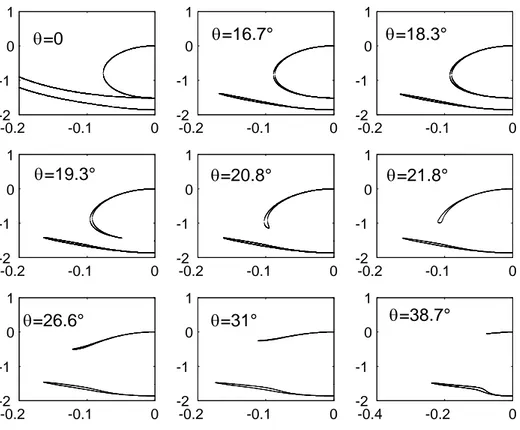
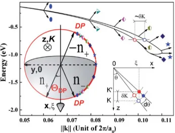
Fig. 1.9 — Evanescent states in the fundamental bangap along the [tan θ, 0, i] direction (where θ = ξ/K, i.e., k = [ξ, 0, iK]) via the 14 × 14 k · p calculation [RDRF]. The presence of the spin-orbit coupling and the lack of an inversion center leads to a splitting in the complex band structure when θ 6= 0.
-0.2 -0.1 0 -2 -1 0 1 -0.2 -0.1 0 -2 -1 0 1 -0.2 -0.1 0 -2 -1 0 1 -0.2 -0.1 0 -2 -1 0 1 -0.2 -0.1 0 -2 -1 0 1 -0.2 -0.1 0 -2 -1 0 1 -0.2 -0.1 0 -2 -1 0 1 -0.2 -0.1 0 -2 -1 0 1 -0.4 -0.2 0 -2 -1 0 1 θ=0 θ=16.7° θ=18.3° θ=19.3° θ=20.8° θ=21.8° θ=26.6° θ=31° θ=38.7°
Fig. 1.10 — 14 × 14 k · p calculation : Evanescent energies are plotted versus the wave-vector modulus ||k|| in 2π/a unit, a is the cubic-lattice parameter. The
k· p parameters used are EG = 1.519 eV, P = 9.88 eVÅ, P0 = 0.41eVÅ, PX =


![Fig. 1.8 — Evanescent states in the forbidden bandgap of GaAs and AlAs in the Kane model [SH].](https://thumb-eu.123doks.com/thumbv2/123doknet/2851193.70614/44.892.277.648.202.506/evanescent-states-forbidden-bandgap-gaas-alas-kane-model.webp)