HAL Id: hal-02084279
https://hal.archives-ouvertes.fr/hal-02084279
Submitted on 12 Nov 2020
HAL is a multi-disciplinary open access
archive for the deposit and dissemination of
sci-entific research documents, whether they are
pub-lished or not. The documents may come from
teaching and research institutions in France or
abroad, or from public or private research centers.
L’archive ouverte pluridisciplinaire HAL, est
destinée au dépôt et à la diffusion de documents
scientifiques de niveau recherche, publiés ou non,
émanant des établissements d’enseignement et de
recherche français ou étrangers, des laboratoires
publics ou privés.
Use of Sobol indexes for efficient parameter estimation
in a charge transport model
Iman Alhossen, Florian Bugarin, Stéphane Segonds, Fulbert Baudoin, G.
Teyssedre
To cite this version:
Iman Alhossen, Florian Bugarin, Stéphane Segonds, Fulbert Baudoin, G. Teyssedre. Use of Sobol
in-dexes for efficient parameter estimation in a charge transport model. IEEE Transactions on Dielectrics
and Electrical Insulation, Institute of Electrical and Electronics Engineers, 2019, 26 (2), pp.584-592.
�10.1109/TDEI.2018.007702�. �hal-02084279�
Use of Sobol Indexes for Efficient Parameter Estimation in
a Charge Transport Model
Iman Alhossen, Florian Bugarin, Stéphane Segonds
Institute Clément Ader, University of Toulouse, ISAE-SUPAERO, IMT MINES ALBI, UPS, INSA, CNRS, 3 Rue Caroline Aigle, 31400 Toulouse, France
Fulbert Baudoin, Gilbert Teyssèdre
University of Toulouse, UPS, INPT, LAPLACE 118 route de Narbonne, F-31062, Toulouse cedex 9, France
ABSTRACT
This article aims at carrying out a parameter sensitivity analysis on a mathematical model for the charge transport in dielectrics, using the Sobol sensitivity method. The main point of the work is to perform a sensitivity analysis under the variation of some impacting experimental factors that are: the temperature, the applied electric field, and the charging time. Useful indications were obtained, coming from studying sensitivity under parameters variation. Indeed, this study helps in revealing the experimental conditions at which each model parameter is the most impacted. Then, , the sensitivity analysis results are used to determine the best starting points for optimization process in order to precisely and rapidly estimate each model parameter.
Index Terms — Dielectrics, charge transport model, optimization, sensitivity analysis
1 INTRODUCTION
V
ARIOUS physical models have been implemented to describe the mechanisms of charge generation and transport in solid dielectrics [1, 2, 3]. These models encompass charge generation, transport, trapping, recombination and take into account the bipolar nature of transport in insulators. They aim at predicting the time dependence of the charge distribution along with external charging and discharging currents, so in a transient regime. Most of the processes involved in this problem are nonlinear in field. Their development combines dielectrics physics inspired from semiconductor physical concepts developed decades ago with more recent numeric techniques for their resolution. In terms of computational approach for the resolution, particle models have been used in some cases as with non-homogeneous materials, for example [4], but in general, fluid models tend to be preferred. Here, the efforts have been put to the selection and implementation of numeric schemes enabling for example to lower numeric diffusion [5, 6]. Usually, parameters pertaining to charge transport model need to be precisely defined. It is the case for mobility, injection barrier, trapping coefficient, etc. However, most of these parameters cannot be determined by independent experiments and it is a heavy task to estimate parameter values that best fit experimental data. Optimization algorithms aim at systematizing this part of the modeling activity. Genetic algorithms for example have been implemented for that purpose [7]; but the computation time can be prohibitive, as the model has to be run with asubstantial number of iterations. To facilitate the convergence of optimization algorithms, it is important to quantify the effect of each input variable on the output observations in order to limit the optimization to the most influential variables set. The method implemented in this work, based on Sobol’s analysis, guides the choice of the optimization algorithms by focusing on the main parameters affecting the charge transport model, which makes possible the resolution within an acceptable time. Particularly, this is done by providing a relevant starting point for each of the optimization processes aiming at determining each of the model parameters This work is presented as follows. In the following section 2, the charge transport model is detailed. Then, section 3 describes how a sensitivity analysis is performed using the Sobol method. Finally, section 4 presents the results obtained for the sensitivity study for the four parameters concerning two main outputs of the charge transport model: charge and current density. Both of these outputs are easily observed using experimental devices.
2 THE CHARGE TRANSPORT MODEL
The model examined here is a unipolar description of charge transport already presented in its bipolar version in [1]. This model considers two levels of charge traps: a deep trap level accounting for relatively long-lasting trapping of charges and a shallow level, which is associated with the effective mobility for mobile carriers. Charge carriers have a given probability to escape from deep traps by overcoming a potential barrier that is included in the de-trapping coefficients. Two kinds of species are considered, mobile and trapped carriers.
Two outputs of this model are investigated in this study: the charge density and the current density. These outputs are estimated using Poisson's equation, continuity equation and transport equation (orientation polarization and diffusion processes are neglected):
( , ) . ( , ). . µ( , ) j x t µ E x t e n x t (1) ( , ) ( , ) ( , ) n x t j x t s x t t x (2) ( , ) ( , ) . E x t n x t e x (3)
The term s x t( , )is the source term. Such equations relate the spatial changes in the current density for a given specie to the changes in carrier concentration through trapping, de-trapping or others physical processes. There are two equations for the source of equation (2): one for the mobile carriers s x t1( , )and one for trapped carrierss x t2( , ):
1 0 ( , ) ( , ) . ( , ). 1 t . ( , ) µ t t n x t s x t B n x t D n x t n (3) 2 0 ( , ) ( , ) . ( , ). 1 t . ( , ) µ t t n x t s x t B n x t D n x t n (4) where:
j x t( , )is the transport current associated with mobile carriers of density n x t and charge e , µ( , )
µ is the mobility,
E x t( , ) is the electric field, n x t mobile carrier density, µ( , ) n x tt( , ) is the trapped carrier density,
( , )n x t n x tµ( , )n x tt( , ) is the total carrier density, B is the trapping coefficient,
n0t is the trap density which verifies in the presented case
3 0
. t 100 .
e n C m ,
D is the de-trapping coefficient which is of the form: . .exp . tr B e w D v k T (5) T is the temperature, wtr is the de-trapping barrier,
1.381 1023
B
k J/K is the Boltzmann's constant, v is the attempt to escape frequency, which has been set
to . 12 1 6.2 10 B k T s h at room temperature.
These equations have a specific form for the interfaces, and they are complemented by boundary conditions (e.g. applied electric field, etc.).
Notably, the charge generation is supposed to result from injection at the electrodes according to a corrected Schottky
law (there is no injection when the electric field at the electrode is null): 2 0( ) ( , ) exp exp 1 4 inj B B eE t ew ew j x t AT k T k T (6) where:
w is the barrier to injection,
E t0( )E(0, )t is the electric field at the electrode,
6 2 2
1.2 10
A Am K , is the Richardson constant. Finally, the material considered in this study is a low-density polyethylene (LDPE) material, in film form of thickness
200
D µm.
3 STATE OF ART IN SENSITIVITY
ANALYSIS
3.1 SENSITIVITY ANALYSIS AND ITS QUANTIFICATION
Consider a mathematical model that uses a set of independent random inputs X (X1,K,Xn) to determine a
random output Y(or response) via a deterministic functionf : : ( ) n f X Y f X a a R R (7)
Practically, f can be very complex (e.g. system of partial differential equations) and usually it is evaluated using a black box (a computer code) which can be time consuming in terms of computation. In different modeling processes, it is essential to determine which inputs contribute most to the output variability and which of them are insignificant so that they can be ignored during first investigation steps.
In this manner, Sensitivity Analysis (SA) has gained a considerable attention, as it assesses how variations in the model output can be apportioned to different input sources. This leads to the determination of how the output is dependent on each of the inputs. Usually SA methods are classified in three groups:
Screening methods [8] that analyze qualitatively the sensitivity of the output. These methods are based on the discretizing of the inputs into levels. They aim at identifying the non-influential inputs using a small number of model evaluations.
Local sensitivity [9] which evaluate quantitatively the impact of a small variation of the input around a fixed value. Each input is varied one at a time, while holding the others at some local values.
Global sensitivity [10] which analyze quantitatively the output variability by varying all the inputs over their whole ranges. This approach is mainly based on the decomposition of the output variance in terms of inputs variances.
Quantitative sensitivity analysis methods usually present sensitivity of the inputs in terms of sensitivity indexes. Since the aim of the present work is to make possible the
determination of an optimally calibrated model, the global Sobol sensitivity method has been chosen in order to ensure an optimization process on the whole variation range of input parameters. The following example places an emphasis on the
sensitivity index.
3.2 PREAMBLE: THE LINEAR MODEL
Suppose that f is linear:
0 1 n i i i Y X
(8)Because the input variables are supposed to be independent, the variance can be written as:
2 1 ( ) ( ) n i i i Var Y Var X
(9) where 2 ( ) i Var Xi is the part of the variance Var Y( ) due to the variableXi. The sensitivity of Y with respect to Xi can be simply quantified by the ratio of the part of the total variance due to Xion the total variance:
2 ( ) 0,1 ( ) iVar Xi Var Y (10)This ratio is usually called Standardized Regression
Coefficient
SRCi
and it represents the part of Var Y( )that is due toXi. In case where f is non-linear, such a coefficient can be calculated using Sobol's method.3.3 SOBOL’S METHOD IN SENSITIVITY ANALYSIS
Now consider a non-linear function f whose analytic form is unknown. The effect of an input variable Xion the output
Ycan be detected by studying the variation of Y if the variable Xi is fixed at some valuexi
, i.e. the conditional variance of Y with respect to Xi is expressed by
( i i)
Var Y X x . Indeed, comparing this conditional variance
to the total variance of Y gives an indication of the impact of
Yon the outputY. If Var Y X( i xi) is approximately equal to Var Y( ) this means that Xi has no significant effect on the output. However, if Var Y X( i xi)is much smaller that
( )
Var Y this means thatXi has an apparent effect on the output. The problem of this indicator is the choice of the valuexi, as
i
X may possesses different values over its range of variation. However, this is solved by considering the expectation over the all-possible values ofXi, i.e. E Var Y X
i
.By considering the total variance formula:
( ) i i
Var Y Var E Y X E Var Y X (11)
So the quantityVar E Y X
i
, instead ofE Var Y X
i
, can be also an indicator for the sensitivity of Ywith respect to the inputXi. However, large values of Var E Y X
i
,compared to Var Y( ), indicate high sensitivity of Xi, while small values indicate less sensitivity.
Thus, sensitivity index for Y with respect to Xi can be defined by:
( ) i i Var E Y X S Var Y (12)This index, which quantifies the sensitivity of the output Y
to the input variableXi, is called first-order sensitivity index by Sobol [11] or correlation ratio by McKay [12]. Note that, in the linear case, SiSRCi. In [11], Si was introduced using the decomposition: 1 0 1 1 1 1 ( , , ) ( ) ( , ) ( , , ) n n i i i n ij i j n n i j n f X X f f X f X X f X X
K K L K (13) with:
0 , , , ( ) ( , ) , ( , , ) , i i i i j i j i j i j i j k i j k i j i j f E Y f X E Y X E Y f X X E Y X X E Y X E Y X E Y f X X X E Y X X E Y X E Y X E Y (14)Thus, the variance of Y can be decomposed as a sum of partial variances: 1 1 1 n n i ij n i i j n V V V V
L K (15) with:
, , , , , , , i i i j i j i j i j k i j k i j i j V Var E Y X V Var E Y X X V V V Var E Y X X X V V V (16)Using this decomposition, it is possible to define the second-order indexes: ij ij
V
S
V
(17)which express the sensitivity of Yto the interaction between i
X and Xj, that is, the sensitivity of Y toXiand Xjwhich is not taken into account in the first order Sobol indexes. Analogously one can proceed for the higher order indexes. For example: ijk ijk
V
S
V
(18)expresses the sensitivity of Yto the interaction betweenXi, j
X and Xk which is not taken into account by first and second order indexes. Note that the sum of all the n indexes is equal to 1 and the closer to 1 an index is, the more important
the variable is. However, the number of indexes (from order 1 to order n), is equal to 2n-1. Thus, calculating and interpreting all the indexes become impossible when n is too large. To overcome this problem, the total sensitivity indexes T
i
S have
been introduced [13]. These indexes, which describe the total contribution of an input Xi(including all its interactions) to the outputY, are defined as the sum of all Sobol sensitivity indexes involvingXi: # 12 i i ij n j i T i j j I V V V S S V
K K (19)where Ii#
U
Ii denotes the union of all the sets of indexes iI containing the indexi. For instance, consider a problem with three input variables, then:
1 12 13 123
T i
S S S S S (20)
In most applications only first order, second order and total indexes are calculated. However, computing these indexes requires the computation of the conditional variance using the model function f . Practically, only numerical methods are used [14, 15] and mainly Monte Carlo approaches. Note that, for a model f with n inputs and an m-sample of the input variables, the estimation of all the sensitivity indexes requires m 2n calls of f . However, estimating only first indexes and total indexes requires m (2n+1) calls of f . Consequently, the best strategy consists in computing first S andi S . If the gap iT
T i i
S Sis important, then second order indexes S are ij
computed. Practically, an estimation of Sobol indexes for a model with less than 10 inputs requires m=10000 samples.
3.4 PRELIMINARY EXAMPLE
Through the example given below, a Sobol sensitivity analysis is presented with application to the flux of injected charge at an electrode defined by equation (7). For this analysis, the injection jinj( , ,T w E0) is seen as a function depending on the temperatureT
273.15 , 373.15K K
, the injection barrier height w
1eV, 2eV
and the electric field atthe electrode 1 1
0 10 . , 100 .
E kV mm kV mm . To follow the
notations introduced above, each of the variables T, w and
0
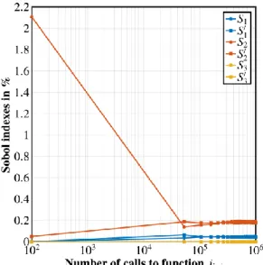
E is denoted respectively byX1, X2andX3. Accordingly, their first order Sobol indexes are denoted byS1, S2 andS3, and similarly the higher order Sobol indexes. Results obtained by sensitivity analysis using Sobol approach are presented in Figure 1.
Figure 1a (respectively 1b and 1c) represents the value of T i
S
(respectively Siand S ) versus the number of evaluations of ij
the injection function. From these three figures, it can be seen that the two values of each index converge after 105 evaluations.
Figure 1d represents as histograms the values of first Si, second S and total indexes ij S . For instance, the first iT
histogram Sirepresents the values ofS1, S2 andS3. From this histogram, it can be concluded that injection is highly sensitive to the injection barrier w and, to a lesser extent, to the temperatureT. However, it is obvious that Siis far from 1 (about 23%) while T
i
S is close to 1. Consequently, the
variability of the injection is highly affected by the interactions betweenT, w andE0. This behavior is confirmed by the S which underlines that the interaction between ij Tand
wplays a predominant role in Var(inj). Indeed, for this case, Sobol indexes are higher than 70% meaning that the contribution of these both parameters induced a great influence on the injection flux. Thus, it is concluded that injection process exists due to the couple temperature and barrier height of injection. Moreover, the high level of Sij
indicates that the interactions between the coupleT E0 and w ,
0
E are negligible. To summarize, the injection function is highly affected by w and the interaction between w andT.
4 PARAMETER SENSITIVITY ANALYSIS
4.1 MODEL AS BLACK BOX
In this application, the charge transport model is viewed as a black box with its input and output. This black box, represented by the function f , includes all the partial differential equations described previously.
The input is represented by a set of physical constants used to describe the mechanisms of charge generation and transport in the solid insulation. In this work, the concerned inputs physical parameters are: the barrier height to injection, mobility of carriers, trapping and de-trapping coefficients (see Table 1).
The output is the main outcomes obtained by the model: charge density (Y ) and current density (1 Y ). Only these two 2
outputs are considered because they are easily observable using experimental devices.
Table 1.Inputs and their ranges of variation Input Notation Unit Lower
Bound
Upper Bound Barrier height for
injection w X1 eV 1.1 1.2 Mobility µ X2 m2.V-1.s-1 10-14 10-12 Trapping coefficient B X3 s -1 5 10-4 10 De-trapping barrier height wtr X4 eV 0.73 1
Table 1 shows the variation range of the set of parameters. The associated ranges of the inputs are specified in order to give a physical sense of the results. Moreover, inputs ranges are kept large enough to ensure a consistent and broad representation of outputs, and thus allowing a tractable computation of the Sobol indexes. Note that the inputs ranges are not unit intervals, so it is assumed that a renormalization
(a) Total indices for Y=jinj(T,w,Elect) (b) First order indices for Y=jinj(T,w,Elect)
(c) Second order indices for Y=jinj(T,w,Elect) (d) Sobol indices for Y=jinj(T,w,Elect)
Figure 1. Sobol indices of different orders of the injection charge as a function of the temperature, injection barrier height and the electric field can be achieved and, after rescaling, each interval is supposed
to be [0, 1]. Accordingly, each input can be conceived as a uniformly distributed random variable over the interval [0, 1], with all the inputs mutually independent.
In order to estimate the Sobol's indexes it is necessary to provide the outputs as scalars. Concerning the outputY , which 1
is normally a net carrier density profile and a function of the position in the insulation and of the time, the scalar is obtained by integrating the net charge over the space and time as follows:
1
pol t D
Y
n dx dt
(21)For the current densityY2, the scalar output is obtained by:
2
pol t
Y
j dt (22)5 RESULTS
Figures 2 to 5 show the evolution of the Sobol indexes respectively for the barrier height to injection, the mobility, the trapping coefficient and the de-trapping barrier height for two different outputs: charge density (full symbols) and current density (open symbols). In each figure, results are obtained based on three protocols applied to a LDPE film of thickness D=200 µm:
First protocol (red curve): Sobol indexes are estimated using data under a DC electric field of 30 kV.mm-1 applied for charging and discharging times of 20 min. The sensitivity analysis is carried out considering that experimental data is acquired over a temperature range of [0, 90°C].
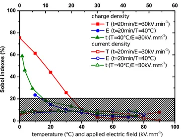
Figure 2. Evolution of the first order Sobol indexes of barrier height to
injection
Figure 3. Evolution of the first order Sobol indexes of the mobility Second protocol (blue curve): Sobol indexes are
estimated using the same material under a temperature of 40°C and for charging and discharging times of 20 min. The sensitivity analysis is realized considering an applied electric field varying over the range [10, 80 kV.mm-1]. Third protocol (green curve): Sobol indexes are estimated under a temperature of 40°C and an applied electric field of 30kV.mm-1. The sensitivity analysis is performed considering charging and discharging times varying over the range [1, 60 min].
In the results analysis, the influence of a given parameter on charge or current density are considered as negligible if the indexes do not exceed 20% (hatched area on the figures). Indeed, a Sobol index below 20% is considered as an indication that the chosen experiment protocol does not give sufficient information to estimate the selected parameter with an optimization algorithm. This is an analysis in relative values of the effect. A low index value mean than other variables of the model contribute more to the output.
5.1 SENSITIVITY ANALYSIS OF BARRIER HEIGHT TO INJECTION
Figure 2 concerns the influence of the barrier height to injection, w in equation (7), on current and charge density.
It appears that, for the model and protocol parameters considered, the barrier to injection does not influence much the current density. For this output, Sobol indexes are below 10% whatever the protocol used. Comparatively, Sobol indexes exceed 50%, meaning a great influence, on the charge density at low temperature (below 30°C) or in charging at short time (less than 10 min). For both cases, it means that the impact on barrier to injection on deposited charge is important.
The fact that this parameter is influential at the beginning of polarization is in phase with the experimental observation. Indeed, when an electric field is applied, charges are injected at the vicinity of the electrodes. The presence of these charges close to the electrode induces a decrease of the electric field at the interface over time and so a decrease of the injection flux. Therefore, the influence over longer times is less important. Roughly, it corresponds to space charge limited process, which also explains why the barrier to injection is not strongly influential on the external current, which corresponds to the space-averaged trapped current [16]. To explain the great influence of the injection barrier on charge density at low temperature it is necessary to have a look at the Schottky law equation (7). This law can be divided into two terms: a term linked to a thermal injection and another term concerning the effect of electric field on the charge injection:
2
Thermal injection term linked to electric field
( , , ) exp exp 1 4 elect inj electrode B B eE ew ew j T w E AT k T k T 1 4 44 2 4 4 43 1 4 4 4 4 2 4 4 4 43 (23)
Results obtained show that thermal injection does not affect so much the charge density at low temperature, only the term linked to the electric field at the injecting electrode is predominant on the charge behavior. At high temperature, the term linked to the electric field becomes negligible, implying
that the temperature effect on the injection current is mainly due to the first term of Schottky law namely the thermal injection effect.
Finally, Figure 2 also shows that the barrier height to injection is not affecting the charge density at T=40 °C, irrespective of the field. Sobol indexes are always below 10%.
5.2 SENSITIVITY ANALYSIS OF THE MOBILITY
Figure 3 concerns the influence of the mobility, µ in equation (1), on the current and the charge density. The indexes are in general low (most of results are in the hatched area) so, according to the results, it seems difficult to find a suitable
experimental protocol for optimization purpose. The temperature seems to be the most influencing both outputs: charge and current density. A temperature higher than 70°C allows having a Sobol index higher than 20%.
To explain this feature, it is necessary to explain more precisely the model of charge transport used. As detailed previously, two kinds of carriers are considered, in this model, being either trapped or mobile and they are provided only by injection at the electrodes. Conduction takes place via a
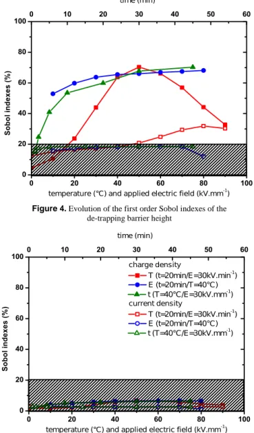
Figure 4. Evolution of the first order Sobol indexes of the
de-trapping barrier height
Figure 5. Evolution of the Sobol indexes of the trapping coefficient constant effective mobility µ, traducing the transport of
carriers through shallow levels that are related to the structural disorder of the polymer. Deep trapping, mainly due to chemical disorder, is described using a unique level of deep traps for each kind of carriers, coefficient B in equation (4) and (5). Charges have a certain probability to escape from deep traps, coefficient D in equation (6), by overcoming a potential barrier, wtr. Based on this physical description,
results show that this model gives more importance to the charges in shallow traps than in deep traps at high temperature. Indeed, for a temperature higher than 70°C, the effective mobility becomes sufficiently sensitive (Sobol indexes exceed 20%) to well estimate this parameter. An explanation could be that at high temperature the fraction of charges in shallow traps is higher.
5.3 SENSITIVITY ANALYSIS OF DE-TRAPPING BARRIER HEIGHT
The results related to the deep trap depth, or de-trapping barrier height, parameter wtr in equation (6) are summarized in
Figure 4. For temperature higher than 50°C, the influence of charge trapping coefficient decreases considering charge density as output. The same happens for the current above 80°C. From room temperature 20°C up to 70°C, the charge density is impacted by the release of charges from deep traps while for a temperature higher than 70°C the charge density is linked to the mobility of charges in shallow traps. For a temperature below 20°C, the charge density is only related to the injection phenomenon, since charges tend to be close to the electrodes and to remain there, Figure 2.
The influence of de-trapping barrier height on charge density increases over time to reach 70% at one hour of charging time for a given temperature of 40°C and a given applied electric field of 30 kV.mm-1. However, this parameter does not influence so much the current density, Sobol indexes are below 10% whatever the protocols used except at high temperature. Thus, it is concluded here that in general, long charging times are preferred for improving sensibility to the de-trapping coefficient.
5.4 SENSITIVITY ANALYSIS OF THE TRAPPING
Figure 5 presents the influence of the trapping coefficient, parameter B in equation (4) and (5), on current and charge density. Very clearly here, this parameter has little effect on the charge or current density. Whatever the protocols used, Sobol indexes are always below 10%. It is not very easy to explain this feature because trapping and de-trapping phenomena are obviously linked by nature.
An explanation could be provided by the equations used where de-trapping phenomenon is modeled with an exponential equation (6) which is not the case for the trapping equation (4) and (5). The difference could also come from the range used for each parameter even if lower and upper bounds are chosen first to be certain to keep physical sense to the conditions, second to have a large range of inputs in order to assume a broad and consistent representation of the output data, and lastly to have tractable computation.
Another key point is to consider the Sobol indexes of order 2. Contrary to the order 1, this order considers mutual interactions of every two inputs.
The results, not shown here, indicate that the mutual interactions between the trapping coefficient and the other parameters gives always a Sobol index less than 20%. In conclusion, considering the windows of experimental protocols (in time, field and temperature) and the observations investigated here (charge density and current) it will be very difficult to estimate this parameter with a good approximation. Last but not least, in the model a fixed trap density is used, as set in previously implemented versions of the model [1, 17, 18]. A part from the fact that this may represent a very low density of defects (3.2 1014 /cm3), it may limit the role of trapped charges in the net charge distribution and in the current. Forthcoming versions of the model should incorporate the possibility that the trap depth can be adjustable.
6 DESIGNING EXPERIMENTS FOR
OPTIMAL PARAMETERS IDENTIFICATION
By analyzing these results, a strategy of study can be designed for parameters optimization. Indeed, optimization algorithms are used to find a set of parameters able to
minimize the deviations between experimental data and simulation data. Experimental data commonly used are the net density of charges as measured by the pulsed electro-acoustic method (PEA) and external charging and discharging current measurements [19]. Simulated data are those produced by the bipolar charge transport model previously explained.
Based on the parameters sensitivity analysis it is possible to find suitable experimental conditions to obtain optimized estimation of parameters used in the studied charge transport model. The measurements are assumed to be realized using a LDPE material, in film form of thickness D = 200 µm, and that the experimental conditions on temperature and field given in section 5 are accessible. Then, according to the analysis, the following guidelines can provide a good approach to estimate the model parameters:
Estimation of barrier height of injection: map of the net charge density under an applied field of 30 kV.mm-1, a temperature of 20°C and charging and discharging times of 20 min.
Estimation of mobility: current measurement with the same experimental protocol than previously except for the temperature of dielectric material that should be higher than 70°C.
Estimation of the de-trapping barrier height: space charge measurement with a temperature from 30°C to 70°C, a field of 30 kV.mm-1 or more; a time of 20 min or more.
Then, the obtained experimental results could be inserted in an optimization algorithm in order to find the new set of parameters. Unfortunately, no straightforward optimal conditions appear for identifying the trapping coefficient. Analysis is in progress to understand why Sobol's coefficients are so low in this case. Recombination processes, and electroluminescence as its pending experimental information, were not incorporated in the model. This could be a route to resolve the uncertainty.
7 CONCLUSION
A global sensitivity analysis, based on Sobol’s method, has been implemented in order to estimate the influence of each parameter of a charge transport model on two main outputs: the charge density and the current density. The procedure has been tested on four variable parameters as model inputs. The approach provides an estimation on the possibility to correctly parameterize the physical model with given observations accessible under a set of experimental conditions. It is shown that the barrier height to injection, for example, is best-estimated considering data at short stressing time whereas the de-trapping barrier height comes out with good confidence at high field/long stressing time. For the trapping coefficient, no ideal conditions on temperature and field could be identified. The reason can be that the trap density is relatively low, in such a way that trapping processes have little impact on the net charge density.
Combined with the results of this global Sobol sensitivity method, an optimization process can be run using different valuable starting points. This is particularly interesting to
ensure speed and accuracy in the convergence of the global optimization process aiming at determining valuable model parameters
REFERENCES
[1] S. Le Roy, G. Teyssedre, C. Laurent, G. C. Montanari and F. Palmieri, "Description of charge transport in polyethylene using a fluid model with a constant mobility: fitting model and experiments," J. Phys. D: Appl. Phys., vol. 39, no. 7, pp. 1427-1436, 2006.
[2] J. M. Alison and R. M. Hill, "A model for bipolar charge transport, trapping and recombination in degassed crosslinked polyethene," J. Phys. D: Appl. Phys., vol. 27, no. 6, pp. 1291-1299, 1994.
[3] J. Xia, Y. Zhang, F. Zheng, Z. An, and Q. Lei, "Numerical analysis of packetlike charge behavior in low-density polyethylene by a Gunn effectlike model," J. Appl. Phys., vol. 109, no. 3, p. 034101, 2011. [4] M. H. Lean, and W. L. Chu, "Simulation of bipolar charge transport in
nanocomposite polymer films," J. Appl. Phys., vol. 117, no. 10, p. 104102, 2015.
[5] J. Tian, J. Zou, and J. Yuan, "Combined RKDG and LDG method for the simulation of the bipolar charge transport in solid dielectrics," PIERS Online, vol. 5, no. 1, pp. 51-55, 2009.
[6] S. Le Roy,G. Teyssedre, and C. Laurent, "Numerical methods in the simulation of charge transport in solid dielectrics," IEEE Trans. Dielectr. Electr. Insul., vol. 13, no. 2, pp. 239-246, 2006.
[7] D. Min, M. Cho, S. Li, and A. R. Khan, "Charge transport properties of insulators revealed by surface potential decay experiment and bipolar charge transport model with genetic algorithm," IEEE Trans. Dielectr. Electr. Insul., vol. 19, no. 6, pp. 2206-2215, 2012.
[8] M. D. Morris, "Factorial sampling plans for preliminary computational experiments," Technometrics, vol. 33, no. 2, pp. 161-174, 1991. [9] T. Turanyi, "Sensitivity analysis of complex kinetic systems. Tools and
applications," J. Mathematical Chem., vol. 5, no. 3, pp. 203-248, 1990. [10] J. Jacques, C. Lavergne, and N. Devictor, "Sensitivity analysis in
presence of model uncertainty and correlated inputs," Reliability Engineering & System Safety, vol. 91, no. 10, pp. 1126-1134, 2006. [11] I. M. Sobol, "Sensitivity estimates for nonlinear mathematical models,"
Mathematical Modelling and Computational Experiments, vol. 1, no. 4, pp. 407-414, 1993.
[12] M. D. Mckay, "Evaluating prediction uncertainty," US Nuclear
Regulatory Commission, Los Allamos, 1995.
[13] A. Saltelli and T. Homma, "Importance measures in global sensitivity analysis of nonlinear models," Reliability Engineering & System Safety, vol. 52, no. 1, pp. 1-17, 1996.
[14] A. Saltelli, P. Annoni, I. Azzini, F. Campolongo, M. Ratto, and S. Tarantola, "Variance based sensitivity analysis of model output. Design and estimator for the total sensitivity index," Computer Physics Communications, vol. 181, no. 2, pp. 259-270, 2010.
[15] I.M. Sobol, S. Tarantola, D. Gatelli, S.S. Kucherenko, and W. Mauntz, "Estimating the approximation error when fixing unessential factors in global sensitivity analysis," Reliability Engineering & System Safety, vol. 92, no. 7, pp. 957-960, 2007.
[16] F. Baudoin, S. Le Roy, G. Teyssedre, and C. Laurent, "Bipolar charge transport model with trapping and recombination: an analysis of the current versus applied electric field characteristic in steady state conditions," J. Phys. D: Appl. Phys., vol. 41, no. 2, p. 025306, 2007. [17] F. Rogti and H. Boukhari, "Numerical modeling of charge transport in
polymer materials under DC continuous electrical stress," Trans. Electr. Electronic Materials, vol. 16, no. 3, pp. 107-11, 2015.
[18] J. Zhao, Z. Xu, G. Chen, and P. Lewin, "Numeric description of space charge in polyethylene under ac electric fields," J. Appl. Phys., vol. 108, no. 12, p. 124107, 2010.
[19] R. Liu, T. Takada, and N. Takasu, "Pulsed electro-acoustic method for measurement of space charge distribution in power cables under both DC and AC electric," J. Phys. D: Appl. Phys., vol. 26, no. 6, 1993.