HAL Id: hal-02055682
https://hal.archives-ouvertes.fr/hal-02055682
Submitted on 8 Dec 2020
HAL is a multi-disciplinary open access
archive for the deposit and dissemination of
sci-entific research documents, whether they are
pub-lished or not. The documents may come from
teaching and research institutions in France or
abroad, or from public or private research centers.
L’archive ouverte pluridisciplinaire HAL, est
destinée au dépôt et à la diffusion de documents
scientifiques de niveau recherche, publiés ou non,
émanant des établissements d’enseignement et de
recherche français ou étrangers, des laboratoires
publics ou privés.
motor timing precision
Laetitia Grabot, Tadeusz Kononowicz, Tom Dupré La Tour, Alexandre
Gramfort, Valérie Doyère, Virginie van Wassenhove
To cite this version:
Laetitia Grabot, Tadeusz Kononowicz, Tom Dupré La Tour, Alexandre Gramfort, Valérie Doyère,
et al.. The strength of alpha-beta oscillatory coupling predicts motor timing precision. Journal
of Neuroscience, Society for Neuroscience, 2019, 39 (17), pp.2473-18.
�10.1523/JNEUROSCI.2473-18.2018�. �hal-02055682�
Behavioral/Cognitive
The Strength of Alpha–Beta Oscillatory Coupling Predicts
Motor Timing Precision
X
Laetitia Grabot,
1*
X
Tadeusz W. Kononowicz,
1*
X
Tom Dupre´ la Tour,
2X
Alexandre Gramfort,
2,3,4Vale´rie Doye`re,
5and
X
Virginie van Wassenhove
11Cognitive Neuroimaging Unit, CEA DRF/Joliot, INSERM, Universite´ Paris-Sud, Universite´ Paris-Saclay, NeuroSpin center, 91191 Gif-sur-Yvette, France, 2LTCI, Telecom ParisTech, Universite´ Paris-Saclay, 75013 Paris, France,3Inria, Universite´ Paris-Saclay, Saclay, 91120 Palaiseau, France,4CEA, Universite´ Paris-Saclay, 91191 Gif-sur-Yvette, France, and5Neuro-PSI, Universite´ Paris-Sud, Universite´ Paris-Saclay, CNRS, 91405 Orsay, France
Precise timing makes the difference between harmony and cacophony, but how the brain achieves precision during timing is unknown.
In this study, human participants (7 females, 5 males) generated a time interval while being recorded with magnetoencephalography.
Building on the proposal that the coupling of neural oscillations provides a temporal code for information processing in the brain, we
tested whether the strength of oscillatory coupling was sensitive to self-generated temporal precision. On a per individual basis, we show
the presence of alpha– beta phase–amplitude coupling whose strength was associated with the temporal precision of self-generated time
intervals, not with their absolute duration. Our results provide evidence that active oscillatory coupling engages
␣ oscillations in
main-taining the precision of an endogenous temporal motor goal encoded in
 power; the when of self-timed actions. We propose that
oscillatory coupling indexes the variance of neuronal computations, which translates into the precision of an individual’s behavioral
performance.
Key words: alpha; beta; cross-frequency coupling; phase–amplitude coupling; time perception; timing
Introduction
Assessing how the brain precisely keeps track of time is typically
complicated when using sensory stimulation, which prevents
dis-entangling endogenous timing brain processes from exogenous
or sensory-driven processes. Using a temporal production task
(
Mita et al., 2009
) helps to bypass this difficulty: participants
self-initiate their endogenous timing by pressing a button, and
press a second time when they considered that the required
du-ration has elapsed. The two actions are internally generated and
driven by an endogenous timing goal independently of any
sen-sory inputs. Recording brain activity between the two button
presses may provide insights on how the brain endogenously
computes time, and self-generates a duration. As in many daily
activities, the goal of reliable temporal production in this task
consists in being accurate (i.e., minimizing the constant error)
and precise (i.e., minimizing the variance).
Here, we explored the role of neural oscillations during the
generation of a time interval in the absence of exogenous
stimu-lation, and tested whether the coupling of neural oscillations was
a signature of the temporal accuracy and/or precision of timed
actions. The relevance of neural oscillations for cognitive
opera-Received Sept. 25, 2018; revised Nov. 23, 2018; accepted Dec. 16, 2018.
Author contributions: L.G., T.W.K., and V.v.W. designed research; L.G., T.W.K., and V.v.W. performed research; L.G., T.W.K., T.D.l.T., A.G., and V.v.W. analyzed data; L.G. and T.W.K. wrote the first draft of the paper; L.G., T.W.K., A.G., V.D., and V.v.W. edited the paper; L.G., T.W.K., V.D., and V.v.W. wrote the paper.
This work was supported by the Paris-Saclay IDEX NoTime to V.D., A.G., and V.v.W., the ERC Starting Grant MINDTIME ERC-YStG-263584 Grant to V.v.W., the ERC Starting Grant SLAB ERC-YStG-676943 to A.G., and the ANR-16-CE37-0004-04 AutoTime to V.D. and V.v.W. The funders had no role in study design, data collection and analysis, decision to publish, or preparation of this paper. Preliminary results of this work were presented at the International
Cognitive Neuroscience workshop (Amsterdam, Netherlands, 2017). We thank Nancy Kopell for her astute comments
on an earlier version of the paper.
The authors declare no competing financial interests. *L.G. and T.W.K. contributed equally to this work.
Correspondence should be addressed to Tadeusz W. Kononowicz at [email protected] or Laetitia Grabot at [email protected].
https://doi.org/10.1523/JNEUROSCI.2473-18.2018 Copyright © 2019 the authors
Significance Statement
Which neural mechanisms enable precise volitional timing in the brain is unknown, yet accurate and precise timing is essential in
every realm of life. In this study, we build on the hypothesis that neural oscillations, and their coupling across time scales, are
essential for the coding and for the transmission of information in the brain. We show the presence of alpha– beta phase–
amplitude coupling (
␣– PAC) whose strength was associated with the temporal precision of self-generated time intervals, not
with their absolute duration.
␣– PAC indexes the temporal precision with which information is represented in an individual’s
brain. Our results link large-scale neuronal variability on the one hand, and individuals’ timing precision, on the other.
tions is largely acknowledged (
Buzsa´ki and Draguhn, 2004
;
Jen-sen and Colgin, 2007
;
Fries, 2015
) and cross-frequency coupling
(
Canolty and Knight, 2010
) may support long-range
communi-cation and integration over distinct spatial and temporal scales
(
Akam and Kullmann, 2014
;
Fries, 2015
). A common form of
oscillatory nesting is the modulation of high-frequency power
[e.g., gamma (␥)] by the phase of low-frequency oscillations [e.g.,
theta (
)]. Robust phase–amplitude coupling (PAC) has been
described (
Tort et al., 2008
,
2009
) and may be involved in the
representation of temporal sequences (
Heusser et al., 2016
),
im-plicated in working memory (
Axmacher et al., 2010
;
Voytek et al.,
2010
;
Lisman and Jensen, 2013
;
Roux and Uhlhaas, 2014
) and in
speech processing (
Canolty et al., 2006
;
Giraud and Poeppel,
2012
). Additionally, the observation that low-frequency
oscilla-tions regulate spike timing in the human brain raised the
hypoth-esis that PAC may provide a temporal code for cognition (
Jacobs
et al., 2007
;
Buzsa´ki, 2010
), but whether such temporal code
in-fluences temporal cognition is unknown. Using a temporal
pro-duction task was expected to provide novel insights on this
question.
Oscillatory coupling could mediate the integration of
infor-mation across temporal scales during interval timing (
Gu et al.,
2015
) so that higher-frequency activity would presumably
inte-grate over the time scales of low-frequency neural activity (
van
Wassenhove, 2016
). The information-theoretic internal clock
(
Treisman, 1963
, for review see
Kononowicz and van
Wassen-hove, 2016
) implies that duration estimation results from the
integration of information (i.e., a count of number of pulses or
events) over time: the high-frequency activity would thus index
pulses generated by the pacemaker, whereas low-frequency
oscil-lations would implement the gating and accumulation of pulses.
A stronger PAC would result in optimal integration of
informa-tion, and linearly predict the generated duration. Alternatively,
oscillatory coupling may implement the maintenance of
task-relevant information in working memory (
Roux and Uhlhaas,
2014
), which would predict a linear association with precision.
PAC may regulate the precision of information during its
main-tenance over relevant brain networks. We thus investigated
whether the temporal precision of motor timing, i.e., the
preci-sion of self-generated time intervals, rely on the temporal
opti-mization of neural information through oscillatory coupling
mechanisms.
To contrast the integration and the precision working
hypoth-eses, we related three distinct aspects of timing behavior with
oscillatory activity recorded with magnetoencephalography
(MEG): performance (the produced duration), accuracy (the
variation of the temporal production relative to the target
inter-val, or constant error), and precision (the variance of temporal
production across trials). The endogenous generation of a time
interval was characterized by robust alpha– beta (
␣–) PAC
ob-servable on a per individual basis. Crucially, the strength of
␣–
coupling correlated with timing precision, but not with the
pro-duced duration itself. Our results support the fundamental role
of oscillatory coupling in the temporal coding of information,
extending this notion to self-generated timing and behavioral
precision.
Materials and Methods
Participants. Nineteen right-handed volunteers (11 females, mean age: 24
years old) with no self-reported hearing/vision loss or neurological pa-thology took part in the experiment and received monetary compensa-tion for participacompensa-tion. Each participant provided a written informed consent in accordance with the Declaration of Helsinki (2008) and the
Ethics Committee on Human Research at NeuroSpin (Gif-sur-Yvette). The data of seven participants could not be included in the analysis because of the absence of anatomical MRI, problems with the head po-sitioning system, abnormal artifacts during MEG recordings, and two participants did not finish the experiment. These datasets were excluded a priori and were not visualized or inspected. Importantly, this harsh procedure did not affect the reliability and power of our statistical assess-ment as most analyses were performed per block, in which a sample for one observation corresponded to⬃100 experimental trials. Additionally, we assessed the power of the linear mixed design where precision was predicted by the␣– PAC, which is the main effect reported in the paper. We performed power analysis using Monte Carlo simulation with 1000 samples, alpha⫽ 0.05, effect size ⫽ 90 (i.e. equal to the effect size re-ported in this paper) using the simr R package. For these parameters, the simulation showed 88% of power, where 80% is considered to be suffi-cient in the literature (Green and MacLeod, 2016). To sum up, this simulation showed that the power in the current study is just in the required range. Hence, the final sample comprised 12 participants (7 females, mean age: 24). All but two participants performed six experi-mental blocks (1 block was removed for 2 participants because of exces-sive artifacts or lack of conformity to task requirements).
Stimuli and procedure. Before the MEG acquisitions, participants were
acquainted with the task by producing 1.45 s duration intervals, and reading written instructions explaining the full experimental procedures. A single trial consisted in producing a time interval followed by the self-estimation of the produced time interval. Feedback varied across blocks (Blocks 1 and 4 included 100% feedback; Blocks 2, 3, 5, and 6 included 15% feedback). Each trial started with the presentation of a “⫹” sign on the screen indicating to participants they could initiate an interval whenever they decided to (Fig. 1A). Participants initiated their
produc-tion of the time interval with a brief button press (R1) when they felt ready to start, and terminated it with another brief button press (R2) when they considered that 1.45 s had elapsed. To initiate and terminate their time production, participants were asked to press the top button on a Fiber Optic Response Pad (FORP; Science Plus Group) using their right thumb. The “⫹” sign was removed from the screen during the estimation of the time interval to avoid any sensory cue or confounding responses in brain activity related to the production of the timed interval. Following the production of the time interval, participants were asked to self-estimate their time estimation using a continuous scale identical to the one used to provide feedback. The intertrial interval between the end of the self-estimation and the first cursor display ranged between 1 and 1.5 s.
Following the completion of the time interval, participants received feedback. A row of five symbols indicated the objective category of the time production tailored to each individual’s time estimation. The feed-back range was set to the value of the perceptual threshold estimated on a per individual basis during a task performed before MEG acquisition (mean population threshold⫽ 0.223 s, SD ⫽ 0.111 s). A near correct time production yielded the middle “⬃” symbol to turn green; a too short or too long time production turned the symbols “⫺” or “⫹” or-ange, respectively; a time production that exceeded these categories turned the symbols “⫺⫺” or “⫹⫹” red. In Block 1, feedback was pro-vided in all trials. In Blocks 2–5, feedback was randomly assigned to 15% of the trials. In Blocks 4 to 6, the target duration was increased to 1.45 s⫹ (individual threshold/2). Feedback was presented in all trials in Block 4 and in 15% of trials in Block 5 and 6, This experimental manipulation was outside the scope of the question in this study, and was addressed in another analysis assessing the possibility of implicit temporal recalibra-tion (cf.Kononowicz et al., 2018). On average, the new target duration was 1.56 s based on the average threshold. In Blocks 1 and 4, participants produced 100 trials; in Blocks 2, 3, 5, and 6, participants produced 118 trials.
Between all experimental blocks, participants were reminded to pro-duce the 1.45 s target duration as accurately as possible, and to maximize the number of correct trials in each block. Note that the manipulation of feedback was investigated in a different set of analyses pertaining to tem-poral metacognition during motor timing (Kononowicz et al., 2018) and does not constitute our condition of interest in this study.
Simultaneous MEG/EEG recordings. The experiment was conducted in
a dimly lit magnetically-shielded room located at NeuroSpin (CEA/DRF/ Joliot) in Gif-sur-Yvette. Participants sat in an armchair with eyes opened looking at a projector screen. Electromagnetic brain activity was recorded using the whole-head Elekta Neuromag Vector View 306 MEG system equipped with 102 triple-sensors elements (2 orthogonal planar gradiometers, and 1 magnetometer per sensor location) and the 64 native EEG system using Ag-AgCl electrodes (EasyCap) with impedances⬍15 k⍀. Participants’ head position was measured before each block using four head-position coils placed over the frontal and the mastoid areas. The four head-position coils and three additional fiducial points (nasion, left and right pre-auricular areas) were digitized using a 3D digitizer (Polhemus) for subsequent coregistration of the individual’s anatomical MRI with brain recordings. MEG and EEG recordings were sampled at 1 kHz, and bandpass filtered between 0.03 and 330 Hz. The electro-oculograms (horizontal and vertical eye movements), electrocardio-grams, and electromyograms were simultaneously recorded. Feedback was presented using a PC running Psychtoolbox software (Brainard, 1997) in MATLAB (R2012, Mathworks).
Data analysis
MEG/EEG data preprocessing. MEG data were low-passed at 160 Hz,
decimated at 333 Hz and epoched from⫺1.2 to 2 s around the first button press (R1). Epochs were rejected if signal amplitudes exceeded 4 fT/cm for gradiometers and 5500 fT for magnetometers. Baseline correc-tion was applied by subtracting the mean value ranging from⫺0.2 to 0 s before R1.
Power density spectrum analysis. The power spectrum density (PSD)
was computed using Welch’s method, between 1 and 45 Hz, with 0.8 s length tapers, on a window from 0.4 to 1.2 s. PSD were averaged across all magnetometers, conditions and participants.
PAC calculation and statistical assessment. Our analysis of PAC
con-ducted in sensor space exclusively focused on activity recorded with mag-netometers; PAC in source space included all sensors (magnetometers, gradiometers, EEG electrodes). We selectively used magnetometers in sensor space for simplicity of interpretation in topographies. Signal source separation in preprocessing stages alleviate the independence of gradiometers and magnetometers; gradiometers would also need to be combined as pairs to make physiological sense and would implicate
ad-ditional difficulties in the computation of phase coupling. We thereafter use the word “sensors” to refer to magnetometers.
To prevent the contamination of the timed interval from both R1- and R2-evoked responses, we solely focused on the time segment from 0.4 to 1.2 s following R1. PAC was assessed using the modulation index (MI;
Tort et al., 2009); namely, the fully epoched data were first bandpass filtered (slow-frequency bandwidth ⫽ 2 Hz, high-frequency band-width⫽ 20 Hz), and then the instantaneous amplitude of the high-frequency and the phase of the slow-high-frequency were extracted from the Hilbert transform applied to the epoch data. The data were then seg-mented into 0.4 to 1.2 s epochs. To assess whether the distributions diverged from uniformity, the Kullback–Leibler (KL) distance was cal-culated then normalized to give the MI. The KL distance was estimated between histograms with 18 bins. The slow-frequency component ranged from 3.5 to 14.1 Hz (step by 0.2 Hz) and the high-frequency range was from 14 to 160 Hz (in step of 2 Hz). A comodulogram was computed for each sensor.
Visual inspection of grand average data across all individuals and sen-sors revealed a strong MI between the phase of␣ oscillations and the power of oscillations. To assess the statistical significance of PAC at the individual level, the MI was compared with a surrogate distribution (n⫽ 100) computed by shifting the low-frequency signal by a minimum of 1 s, as has been previously proposed (Tort et al., 2010). To reduce computa-tional demands, this procedure was only performed on 10 selected sen-sors per individual, based on the maximal␣– MI value (8–12/15–40 Hz) across all conditions. It should however be noticed that the selection process is independent from the main contrasts-of-interest concerning behavioral accuracy and precision. A Z-score was calculated for each of the 10 selected sensors and a Z-score⬎4 (i.e., p ⫽ 3e⫺5) was reported as significant.
The problem of multiple comparisons while computing PAC has been rarely discussed or acknowledged. We note that controlling for multiple comparisons would necessitate correction of 0.05 by 3869 (number of cells in the MI matrix)⫻ 102 (number of sensors) number of compari-sons, which would result in 1.27.e⫺7 (i.e., Z-score of 5.28). Sufficient evidence for PAC not confounded by multiple-comparisons problem can be gathered by inspection of the Z-score values inFigure 3A, which
reached values⬎20th Z-score corresponding to 5.6e⫺89 p value.
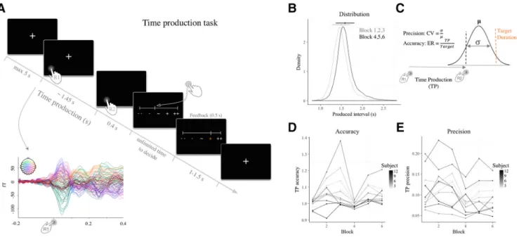
Figure 1. Probing behavioral precision (CV) and accuracy (ER) using a time production paradigm. A, Time course of an experimental trial. Participants received feedback on their performance for all trials in Blocks 1 and 4, and for 15% of trials in Blocks 2, 3, 5, and 6. The inset plot depicts the evoked MEG responses locked to R1. B, Probability density function of all TP when producing 1.45 s (gray) and 1.56 s (black). The dots and bars indicate their respective means and SD. C, Schematic depiction of how temporal precision and accuracy were quantified. The black dotted line depicts an example of a produced time interval drawn from a Gaussian distribution of produced intervals (solid black curve; meanandSD).Thenextpanelsplottheprecisionandtheaccuracyacrossblocks and participants. D, Accuracy in time production computed as ER (⫽ production/target) per block and per individual (dot). The accuracy of TP did not significantly change in the course of the experiment. E, Temporal precision computed as CV over time productions per block and per individual (dot). The temporal precision of TP did not significantly change in the course of the experiment.
To assess whether PAC was specific to time production, we compared the MI computed during baseline from⫺0.8 to 0 s before R1 to the MI computed during the produced interval (0.4 to 1.2 s). Because partici-pants were allowed to begin the task when ready after the display of the cross, we selected trials with at least 1.1 s between the cross onset and the first button press (R1) to avoid any contamination of visual-evoked ac-tivity. On average 90⫾ 80 trials were retained. For three participants, the number of trials was not sufficient to compute a reliable MI (6, 15, and 21 trials). Nevertheless, the cluster-based permutation t test was run on all individuals and similar results held when the same analysis was per-formed on nine participants.
Crucially, because of methodological limitations inherent to the filter-ing process, PAC can only be established for a driver’s frequency that is above twice the frequency of the high-frequency oscillations. To insure that the␣ and  frequencies involved in the oscillatory coupling were not harmonically related, we extracted, per individual, the␣ and  frequen-cies corresponding to the maximal MI averaged across the 10 selected sensors of each participant. We then ran a paired t test between the frequency and the second harmonic of the␣ frequency to insure that the coupling was not spurious. The outcomes of these analyses are detailed in Results.
MEG/EEG-aMRI coregistration. Anatomical magnetic resonance
im-aging (aMRI) was used to provide high-resolution structural images of each individual’s brain. The anatomical MRI was recorded using a 3-T Siemens Trio MRI scanner. Parameters of the sequence were as follows: voxel size: 1.0⫻ 1.0 ⫻ 1.1 mm; acquisition time: 466 s; repetition time ⫽ 2300 ms; and echo time⫽ 2.98 ms. Volumetric segmentation of partic-ipants’ anatomical MRI and cortical surface reconstruction was per-formed with the FreeSurfer software (http://surfer.nmr.mgh.harvard.edu/). A multiecho FLASH pulse sequence with two flip angles (5° and 30°) was also acquired (Fischl et al., 2004;Jovicich et al., 2006) to improve coreg-istration between EEG and aMRI. These procedures were used for group analysis with MNE software (Gramfort et al., 2013,2014). The coregis-tration of the MEG/EEG data with the individual’s structural MRI was performed by realigning the digitized fiducial points with MRI slices. To ensure reliable coregistration, an iterative refinement procedure was used to realign all digitized points with the individual’s scalp.
MEG source reconstruction for PAC analysis. To compute PAC at the
source level, single-trial time series were projected into source space. All three types of sensors were combined: magnetometers, gradiometers, and EEG signals. Before the main source reconstruction, individual for-ward solutions for all source locations on the cortical sheet were com-puted using a three-layer boundary element model constrained by the individual’s anatomical MRI. Cortical surfaces extracted with FreeSurfer were downsampled to 10,242 equally-spaced sources on each hemisphere (3.1 mm between sources). The noise covariance matrix for each indi-vidual was estimated using baseline activity (interval from⫺0.2 to ⫺0.1 s relative to R1). The forward solution, the noise covariance and source covariance matrices were used to calculate the dSPM estimates (Dale et al., 2000). The inverse computation was done using a loose orientation constraint (loose⫽ 0.2, depth ⫽ 0.8) on the radial component of the signal. Individuals’ current source estimates were registered on the Free-Surfer average brain for surface-based analysis and visualization. Once time-resolved activity was reconstructed in cortical space, we used the “aparc” parcellation from FreeSurfer to define cortical labels (Desikan– Killiany atlas;Desikan et al., 2006). Given the large number of dipoles within a label, and to reduce computational demands, we reduced each label to five vertices based on either maximal␣ or  power, so that the selection process was independent of PAC. We then computed PAC for each of these selected vertices and averaged it for each label. The corre-lation analyses were then carried on these selected vertices. As seen in
Figures 3C and9C, both selections yielded very comparable results. To
prevent signal cancelation originating from different dipoles, the label time courses were treated as single trials for PAC computation.
Experimental conditions and correlation analyses. Analyses were
per-formed on the basis of objective performance in time production classi-fied as short, intermediate, or long separately for each experimental block. Computing these three conditions within a block focused the analysis on local variations of brain activity as a function of the observed
participant’s performance with respect to the mean temporal production of each participant. Epochs were concatenated across all six blocks for the analyses based on time production performance. The number of trials was equalized between short, intermediate and long conditions, leading to 168 trials (SD⫽ 58) per condition. Additionally, the correlational analyses investigating precision and accuracy of timing processes was also extended to a per block analysis to gain a better insight of the fluc-tuation of these behavioral components over time. Precision was computed as coefficient of variation (CV) over time production on a per-block and per-participant basis. The CVs were calculated by dividing the SD by the mean duration production. Accuracy was quantified by the error ratio (ER): ERs were calculated by dividing the mean temporal production in a given set of data by the target interval in that set. It is important to note that precision and accuracy provide two distinct in-sights on individuals’ temporal production. Although precision is uniquely described in reference to each individual’s temporal produc-tion, the accuracy is computed in reference to the objective target dura-tion. As such, both measures are complementary and not necessarily correlated. The target duration was 1.45 s in the first three blocks and 1.56 s in the last three blocks.
The sensor-level analyses were performed using linear mixed-effect (LME) models and model comparison to check whether factors other than PAC were needed to explain motor timing behavior. Correlational analyses of source estimates were performed for illustrative purposes and thus, we used nonparametric Spearman’s for each label. All statistical analyses were performed in R v3.3.2 statistical programming language (R Core Team, 2016). For illustrative purposes, correlations in cortical space were computed using Spearman correlations. Bayesian ANOVA (Rouder et al., 2012) was performed using BayesFactor R package.
Calculating precision and accuracy metrics and accounting for inflated degrees of freedom. As described above, both precision (CV) and accuracy
(ER) metrics were computed separately per block and per participant. As splitting the data per block and per individual could inflate the degrees of freedom, we used LME models (Pinheiro and Bates, 2000;Gelman and Hill, 2007), which, by default, accounted for individual, multiple per-subject observations in the data. For all regression analyses of sensor data, we used LME models. LMEs are regression models that model the data by taking into consideration multiple levels. Subjects and blocks were en-tered in the model as random effects that were allowed to vary in their intercept. P values were calculated based on a type-3 ANOVA with Sat-terthwaite approximation of degrees of freedom, using lmerTest package in R (Kuznetsova et al., 2017). The mixed-effects models approach was combined with model comparison, which allowed for evaluating the best fitting model in a systematic manner.
Data standardizing for regression model. As regression tests require a
Gaussian distribution of the data, wherever applicable, and on the basis of Shapiro–Wilk normality test, the data were transformed using the Lambert W function. The Lambert W function provides an explicit in-verse transformation, which removes heavy tails from the observed data (Goerg, 2011,2015). First, the data were transformed into a heavy-tailed form using log-likelihood decomposition. Subsequently the heavy-tailed form was transformed back into a Gaussian distribution. All transforma-tions were performed using LambertW R package.
Results
Behavioral evidence for variable precision and accuracy
Twelve participants were asked to produce a target interval by
pressing a button at the start (R1) and at the end (R2) of their
time production (TP;
Fig. 1
A). The target interval was 1.45 s in
the first three experimental blocks, and 1.56 s in the last three
experimental blocks. Participants complied with the task
require-ments by producing, respectively, 1.513 and 1.614 s time intervals
(
Fig. 1
B). Although the overall performance was quite accurate,
the time production data showed large variability both
within-individuals (across blocks) and across within-individuals (
Fig. 1
D, E).
(
Fig. 1
D): the CV was calculated by dividing the SD by the mean
duration production, and the ER by dividing the mean time
esti-mates by the target interval in a given block (
Fig. 1
C). The CV was
thus a measure of precision, and the ER, a measure of accuracy.
Both metrics were calculated per experimental block and per
participant. Although changes in feedback were manipulated in
the experimental design, there was no ad hoc hypothesis
regard-ing its effects on possible PAC, notably because no significant
changes in precision were found as a function of feedback
(repeated-measures ANOVA; F
(5,65)⬍ 1, p ⬎ 0.1). Additionally,
as can be seen in
Figure 1
D, a general trend for a lengthening in
duration estimation was observed over the entire course of the
recording (repeated-measures ANOVA; F
(5,65)⫽ 2.71, p ⫽
0.028); this drift was shown to be independent from changes in
feedback or duration (
Kononowicz et al., 2018
). In the next
sec-tion, we explore the role of oscillatory coupling in timing.
Robust
␣– coupling during time production
Before proceeding with PAC estimations, we assessed the PSD
during the time interval from 0.4 to 1.2 s following R1 (to avoid
motor-evoked responses) by averaging the PSD across all sensors,
conditions, and individuals. A dominant peak was readily visible
in the spectrum at␣ (⬃10 Hz) frequency, suggesting the existence of
plausible regime for oscillatory coupling (
Fig. 2
A). The
␣ peak was
mainly localized in occipital and parietal regions (
Fig. 2
B,C).
To assess whether any form of PAC
was present during the production of a
time interval, we computed the MI (
Tort
et al., 2009
) for all sensors from 0.4 to 1.2 s
following the first button press R1. Visual
inspection of grand average data across all
individuals and all sensors revealed a
strong MI between the phase of
␣
oscilla-tions and the power of
 oscillations in
centro-parietal sensors (
Fig. 3
B). For
di-mensionality reduction, we then selected
10 sensors displaying the maximal
␣–
MI on a per individual basis: as seen in
Figure 3
A, the 10 sensors with maximal
␣– MI were mainly found in central and
parietal regions for a majority of
partici-pants. For each of these selected sensors,
the statistical significance of the MI was
assessed at the individual level by shuffling
the
␣ phase (
Tort et al., 2010
). A Z-score
⬎4 (p ⬍ 0.0001;
Fig. 3
A shows individual
outlines) indicated that
␣– PAC was
sta-tistically significant for each individual.
Across participants,
␣– MI was maximal
for the phase of the 10.3 Hz peak frequency
response (SD
⫽ 0.6), and for the amplitude
of the 27.2 Hz peak frequency response
(SD
⫽ 3.9). For a detailed report,
Table 1
provides all individual frequency peak
re-sponses. Both the low- and high-frequency
peak values were consistent with the
indi-viduals’
␣ and  frequency peaks observed
in the previous PSD (
Figs. 2
,
3
;
Table 1
).
Specifically, we observed that an
individu-al’s
␣ peak frequency correlated with the ␣
peak frequency of the individual’s PAC (r
⫽
0.763, p
⫽ 0.004; see
Fig. 4
).
Importantly, the
 peak in ␣– PAC
was significantly distinct from the second harmonic of the
␣
peak in the
␣– PAC [t ⫽ 7.064, df ⫽ 11, p ⬍ 0.001; CI
95⫽
(4.5; 8.6)], meaning that the observed
␣ and  peak
frequen-cies were not simply harmonics. Although this observation
showed that the observed
 activity was true neuronal activity
(and not harmonics of
␣), it did not directly test whether PAC
was artifactual. Later quantitative assessments testing the
pre-cision in temporal production will directly rule out the
possi-bility that PAC is artifactual. To ensure the robustness of our
observations, we confirmed these results with an alternative
method to quantify
␣– PAC capitalizing on a recently
devel-oped driven auto-regressive (DAR) statistical modeling
ap-proach (
Dupre´ la Tour et al., 2017
). DAR modeling revealed a
comparable
␣– PAC at the individual level (
Figs. 3
,
5
).
To further assess which brain regions may exhibit the highest
degree of coupling, we source-estimated PAC in cortex. First, we
reconstructed the time-resolved signals on a single-trial basis,
and used the same approach for PAC calculation as we did for the
sensor data. We spatially defined brain regions using a predefined
cortical parcellation (Desikan–Killiany atlas;
Desikan et al., 2006
)
and reduced each label to five vertices showing maximal
␣ power
(see Material and Methods).
␣– PAC was maximal in left
sen-sorimotor regions, presumably because of the motoric
compo-nents of the task (post-, pre-, para-central, and supramarginal
Figure 2. Oscillatory power in brain activity during time production. A, The PSD was computed during the produced interval (0.4 –1.2 s) and averaged across sensors, conditions and participants. The average PSD (thick line) across individuals (gray lines) showed a clear peak 10 Hz. The topo map shows the PSD averaged between 8 and 12 Hz. B, The individual topographic maps for PSD. C, Grand-average cortical source estimations revealed an occipito-parietal distribution of the oscillatory power.
areas;
Fig. 3
C). High PAC was also found in parietal regions, in
line with the notion that endogenous
␣ rhythms would largely
contribute to PAC. The
␣ peak analysis (
Fig. 2
C) and the PAC
source estimation (
Fig. 3
C) were thus topographically consistent
with each other. To test the robustness of source estimations, we
also conducted the analysis with a selection of spatial location
based on the maximal
 power: the left sensorimotor areas
showed maximal
␣– PAC, consistent with the ␣-based
observa-tions (
Fig. 3
C, bottom).
Figure 3. ␣– PAC during time production. A, Individual comodulograms showing the presence of significant ␣– PAC as measured by the MI. The individual topographic maps (insets, top
right; nose on top) provide the spatial distribution of the␣– MI observed at the scalp level: 10 sensors showing the highest MI (inset, white dots) were selected for the comodulogram. The white outlines on the individual comodulograms delineate significant Z-scored values (values⬎4, i.e., p ⬍ 0.0001). B, Grand average comodulogram across all trials, all participants, and all sensors, showing significant␣–PAC.Theaveragetopographicmapofthe␣–MI(inset,topright)sharesthesamescaleasinA.C,Z-scoreMIsweresource-reconstructedincortex.Brainregionsshowing maximal MI as computed on the basis of␣ (top) or  (bottom) power are reported.
Figure 4. Individual␣peakfrequency(iAPF)correlateswith␣frequencyobservedin␣– PAC. To ensure that the␣ rhythm captured in the PSD (Fig. 2A) was involved in PAC
computa-tion, we correlated an individual␣ peak frequency with the frequency corresponding to each individual’s maximal␣– MI (r ⫽ 0.763, p ⫽ 0.004).
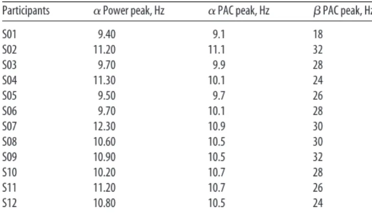
Table 1. Individual␣ peak frequency extracted from the PSD and individual ␣– PAC corresponding to their maximal MI
Participants ␣ Power peak, Hz ␣ PAC peak, Hz  PAC peak, Hz
S01 9.40 9.1 18 S02 11.20 11.1 32 S03 9.70 9.9 28 S04 11.30 10.1 24 S05 9.50 9.7 26 S06 9.70 10.1 28 S07 12.30 10.9 30 S08 10.60 10.5 30 S09 10.90 10.5 32 S10 10.20 10.7 28 S11 11.20 10.7 26 S12 10.80 10.5 24
␣– Coupling is specific to the interval being timed
Although we showed that
␣– coupling was present during the
production of temporal intervals, one may argue that the
ob-served coupling was strictly relevant to motor preparation as
opposed to motor timing. To test this, we capitalized on our
experimental design, which required that participants
self-initiated the production of the time interval: because participants
volitionally initiated their first button press (R1) with no explicit
time requirement or pressure, we used brain activity ranging
from
⫺0.8 s to R1 as a control for motor preparation. We tested
whether the MI during the production of the time interval was
significantly increased compared with this baseline brain
re-sponse (before R1). A cluster-based permutation t test on
co-modulograms averaged across the selected sensors and across
participants showed that
␣– PAC was significantly larger during
time production than during the volitional trial initiation ( p
⫽
0.037;
Fig. 6
). As the number of trials for PAC estimation was not
optimal for three participants, the cluster permutation test was
repeated for the nine participants with a sufficient number of
trials for statistically robust estimation (⬎40 trials), confirming a
PAC significantly larger than in baseline ( p
⫽ 0.016).
Impor-tantly, because the power of the low-frequency oscillation may
impact the MI (
Dupre´ la Tour et al., 2017
), we also insured that
␣
power density did not differ before the time interval and during
Figure 5. ␣– PAC during time production computed with DAR model. We replicated the individual results of ␣– PAC (Fig. 3A) using a novel DAR model (Dupre´ la Tour et al., 2017). The full comodulograms of Z-scored DAR values are plotted for each individual. Topographic maps of␣– DAR values are plotted in the right insets. The white contour corresponds to Z-score values ⬎4 highlighting significant oscillatory coupling. In the DAR approach, and for consistency in comparing results, we kept the same set of sensors as inFigure 3A. For instance, in participant S02, the sensors
showing maximal PAC with Tort’s method (highlighted in white in the topographic inset) did not match with the sensors showing maximal PAC with DAR models; this spatial discrepancy explains why no significant␣– PAC is observed in the comodulogram of S02 despite significant coupling (yellow DAR values on the topographic insets). The DAR method provided a narrower focus on higher frequencies of power modulation, suggesting slightly larger specificity of high-power modulation. It is noteworthy that for both the Tort and the DAR methods, the peak of the high-frequency (Tort method⫽ 27.2 Hz, SD ⫽ 3.9; DAR method ⫽ 34.5 Hz, SD ⫽ 2.3) were located in the vicinity of the and lower ␥ frequencies. This suggests that for every ␣ cycle at least one cycle of  was transiently modulated by the phase of␣ oscillation. As reported in Results, the peak frequencies for ␣ and  found in the ␣– PAC with the DAR method showed no harmonic relationship [t ⫽ 18.641, df⫽ 11, p ⬍ 0.001, CI95⫽ (11.1; 14.0)].
the production of the time interval ( p
⬎ 0.1), and that the
␣–
power ratio did not significantly differ between these two time
periods ( p
⬎ 0.1). In sum, these controls showed that the
␣–
coupling could not be explained by a simple power difference
between the two equivalent motor preparation time periods.
To put our findings in context, it is noteworthy that in a study
requiring similar motor demands (
de Hemptine et al., 2015
), the
strength of PAC was shown to decrease during motor preparation
compared with the time period of the movement; here, during a
timing task, we found the opposite pattern. Altogether, our
com-parisons against baseline showed that the observed
␣– PAC was
likely linked to the task requirements of endogenously producing
a time interval, and thus that
␣– PAC could play a functional
role in temporal performance, which we explored next.
No monotonic associations between oscillatory coupling
strength and time estimation
Under the first working hypothesis, if PAC mediated the
integra-tion of informaintegra-tion across temporal scales during timing, the
coupling strength would be associated with the length of the
pro-duced duration. To directly test whether the generation of a time
interval resulted from the online integration of endogenous
information mediated by oscillatory coupling, we investigated
whether the strength of
␣– PAC predicted timing behavior in an
absolute manner between trials. For this, and in line with
com-mon practice (
Kononowicz and Van Rijn, 2011
), epochs were
sorted as a function of participants’ performance; namely, short,
intermediate, or long duration productions. The
␣– MI was
averaged across selected sensors for each individual and for each
produced duration (
Fig. 7
). A one-way repeated-measures
ANOVA conducted with produced duration as factor (3 levels:
short, intermediate, long) revealed no significant differences in
the strength of
␣– PAC as a function of duration (F
(2,11)⫽
0.657, p
⫽ 0.528). To further investigate the likelihood of the null
hypothesis, we ran the same analysis with Bayesian ANOVA: a
Bayes Factor of 0.29 indicated that the data were 1/0.29
⫽ 3.4
times more likely to occur under the null hypothesis than under
the alternative hypothesis, providing “substantial” (
Jeffreys,
1961
) or “moderate” (
Lee and Wagenmakers, 2014
) evidence
that the strength of
␣– coupling were independent of absolute
timing performance.
As no change in
␣– coupling strength was found as a
func-tion of the produced time interval, we instead asked whether the
phase relationship between
␣ and  changed as a function of the
produced time interval. To test this, epochs were locked on
the peak of the
␣ oscillations (
Fig. 8
) to compare whether
maxi-mal beta power (15– 40 Hz) was found at different phase of the
␣
oscillation as a function the produced time interval. No
signifi-cant changes in the phase relationship between
␣ and the  power
were observed (
Fig. 8
A). Overall, we found that for four
partici-pants, an increase in
 power occurred during the ascending
slope of the
␣ oscillation, and for the remaining eight
partici-pants, at the descending slope of the
␣ oscillation. When looking
at the individual
␣ phase distribution at which  power was
max-imal for each duration category, a large interindividual variability
could be observed (
Fig. 8
B). When comparing the mean phase
relationship between
␣ and  power during short and long
tem-poral intervals, no significant differences were found (t
⫽ 0.12,
p
⫽ 0.91;
Fig. 8
C).
Hence, and overall, the length of the temporal production did
not significantly influence the strength or the phase relationship
of
␣– coupling. These observations land no substantial support
for the direct implication of
␣– PAC in time estimation per se,
and we thus turned to our second working hypothesis.
The strength of
␣– PAC indexes timing precision
Under the precision working hypothesis, oscillatory coupling
may reflect the precision with which an endogenous timing goal
may be maintained during motor production. To test this, we
quantified how the observed
␣– PAC related to participants’
timing accuracy and precision. The
␣– MI were averaged across
sensors separately for each individual, and for each experimental
block, and entered as predictors in two regression models; the
precision (measured by CVs) and the accuracy (measured by
ERs) models.
First, we found that the strength of
␣– oscillatory coupling
significantly predicted the behavioral CV (t
(64)⫽ 3.3,
 ⫽ ⫺89,
p
⫽ 0.002;
Fig. 9
A). The statistical analysis, based on Akaike
information criterion (AIC;
Wagenmakers and Farrell, 2004
),
showed that the model containing
␣– PAC as predictor was
justified compared with the model including only the intercept
(
⌬AIC ⫽ 7.5, p ⫽ 0.002). Inclusion of the interaction of
␣– PAC
with block as a fixed effect in the model was not warranted
(
⌬AIC ⫽ ⫺3, p ⬎ 0.1, respectively). This indicated that despite
variability in behavioral performance, the relationship between
the behavioral precision as quantified by CV (
Fig. 1
E) and the
strength of the
␣– PAC was sustained throughout the entire
experimental session. The lack of interaction precluded the
pos-sible confounding contribution of motivational or attentional
effects typically observed as “time-on-task” effects. To further
test whether PAC indexed the precision of behavioral
perfor-mance, we assessed whether transitions in the strength of
␣–
PAC between blocks (⌬PAC) could predict transitions in
behav-ioral precision between blocks (
⌬CV). For this, we subtracted the
CV and the
␣– MI between consecutive blocks (i.e., Block 2 ⫺
Figure 6. ␣– PAC is specific to the timed interval R1–R2. To ensure that ␣– coupling
was related to endogenous timing processes, we contrasted PAC during temporal production (R1–R2 period) with PAC during the motor preparation to R1 of the same trial (⫺0.8stoR1).All participants (n⫽12)wereincludedinthisanalysis.Thestrengthof␣–PACwassignificantly higher during the time production interval compared with motor preparation during the self-initiation of the time interval. The white line delineates a significant cluster corresponding to
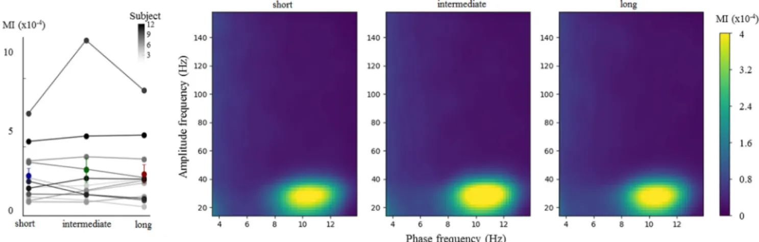
Figure 7. The strength of␣– coupling does not index absolute time production. Trials were split according to the length of the temporal production (left graph: gray, individual data; blue, green and red, mean and SEM for short, intermediate and long trials, respectively). A significant and comparable MI was found suggesting comparable␣- coupling whatever the length of the produced interval.
Figure 8. The relation between␣ phase and  power does not predict the length of produced temporal intervals. A, The time series were locked on the peak of the ␣ oscillations (bottom, dark line, SD marked by dashed lines) and beta power (15– 40 Hz) were computed for each duration. For illustration, the time-frequency phase-locked to the␣peakisshownfortheMEGsensorshowing maximal␣–MIforonerepresentativeparticipant(S06).B,The␣phaseatwhichpowerwasmaximalwasextractedforeachparticipant(circularhistogram)andeachdurationcategory(blue, short; green, intermediate; red: long). C, The␣ phase difference between long and short temporal productions at which  power was maximal was plotted for each participant. The length of the bar represents the number of participants with the same phase value. A Rayleigh test indicated that the phase difference between long and short categorizations was not uniform ( p⬍ 0.02, mean⫽1.4°),confirmingasignificantphaseconcentrationwhenbetapowerwasmaximal.However,themeanphasedifferencebetweenlongandshortdurationdistributiondidnotsignificantly differ (t⫽ 0.12, p ⫽ 0.91), providing no evidence for a different␣– phase relationship as a function of endogenous timing.
Block 1, Block 3
⫺ Block 2, etc.) and showed, in line with the
results of the first model, that
⌬PAC significantly predicted ⌬CV
(t
(51)⫽ 2.6,
 ⫽ ⫺77, p ⫽ 0.012;
Fig. 9
B). This observation
indicated that changes in precision (CV) between blocks could be
accounted for by changes in the
␣– coupling strength between
blocks.
Previous studies on cross-frequency coupling have indicated
that PAC estimation could be confounded during the estimation
of phase and power frequencies (
Aru et al., 2015
). To thoroughly
assess whether the predictive power of PAC strength with respect
to behavioral CV was exclusive to oscillatory coupling, and not
confounded by the power in
␣ or  bands, we tested whether the
inclusion of
␣ power (
Fig. 10
A),
 power (
Fig. 10
B), and
␣–
power ratio (
Fig. 10
C) was justified in the model predicting CV.
We confirmed that the inclusion of
␣, , and ␣– ratio were not
justified in the model predicting CV (⌬AIC ⫽ 1.2, p ⬎ 0.1;
⌬AIC ⫽ 1.8, p ⬎ 0.1; ⌬AIC ⫽ ⫺2.9, p ⬎ 0.1; respectively). The
lack of predictability of precision by
␣ and  power further
sup-ports that PAC is correlated with the precision in temporal
performance, but also indicates that PAC is not caused by
non-sinusoidal waveforms of
␣ and/or  oscillations.
These series of tests were methodologically important to
in-sure the biological reality and interpretation of PAC in our data.
Indeed, the lack of correlation not only strengthened our
previ-ous observation that
 oscillations were not harmonics of ␣ but
further supported the notion that PAC was not caused by
non-sinusoidal waveforms of
␣ and/or  oscillations (
Cole and
Voytek, 2017
). In other words, these tests do not provide
evi-dence for spurious PAC (
Fig. 10
).
Finally, we investigated the association between PAC and
the precision of temporal behavior by correlating the values of the
␣– MI obtained in each highlighted cortical region with the
CVs: significant correlations between
␣– MI and CV were
found in the left motor cortices, in the left supramarginal gyrus,
and in the occipito-parietal regions (
Fig. 9
C). Notably, the left
supramarginal gyrus and pars orbitalis were conjointly seen in
the
␣-based and in the -based selection of vertices. The
impli-cation of these structures in the current timing task is consistent
with previous reports (
Coull et al., 2004
;
Livesey et al., 2007
;
Wiener et al., 2010
).
The strength of
␣– PAC and the power of ␣ index
temporal accuracy
The strength of
␣– PAC was shown to correlate with the
preci-sion of temporal production (CV) across blocks with a stronger
coupling indicating a smaller variance in time production. After
investigating the ad hoc hypothesis proposing that PAC could
regulate the precision of information processing, we assessed
whether
␣– PAC was also related to the differences between
produced time intervals, and the objective target intervals, i.e., to
the accuracy quantified as ERs.
The ER indicated the distance of participants’ temporal
pro-duction from an ideal observer’s performance (
Fig. 1
D). We
found that the strength of
␣– PAC was approaching significance
in predicting ER (t
(58)⫽ 1.9,
 ⫽ ⫺44, p ⫽ 0.058;
Fig. 11
). The
AIC analysis showed that the model containing the strength of
␣– PAC as predictor was marginally justified compared with the
model including only the intercept (⌬AIC ⫽ 1.7, p ⫽ 0.055). No
interaction between the strength of
␣– PAC and block as fixed
effect was found (⌬AIC ⫽ 2.8, p ⬎ 0.1) by comparing a model
with
␣– PAC as a single predictor and a model in which
inter-action with block was added. This result signified that the changes
in behavioral feedback to the participant did not affect the
strength in
␣– coupling. This was further verified by directly
contrasting blocks containing feedback on all trials (100%
feed-back) with blocks in which participants received feedback in only
15% of the trials. The inclusion of feedback in the model was not
warranted (⌬AIC ⫽ 0.5, p ⬎ 0.1). It thus appeared that the
rela-tionship between the observed oscillatory coupling strength, as
measured by
␣– PAC, and the accuracy of time estimation, as
measured by ER, remained stable throughout the entire
experi-mental session.
Finally, to assess the relative contribution of precision and
accuracy in relation to
␣– PAC, we performed a series of model
comparison with precision and accuracy as predictors, again
keeping the same random structure as in the previous statistical
Figure 9. The strength of␣–PACindexestheprecisionoftemporalperformance.A,Overallexperimentalblocksandparticipants,CVsoftemporalproductionweresignificantlycorrelatedwith the strength of␣–PAC.Additionally,␣orpowershowednoindependentcontributiontoCV(Fig. 10), suggesting that␣–PACexclusivelyaccountedforparticipants’temporalprecision.The shaded area around the regression line indicated standard error. B, The relative changes in CV and␣–PACwerecorrelatedwhenparticipantsswitchedfromoneblocktoanother,suggestingthat the transitions in␣– coupling strength were associated with transitions in CV between blocks. The shaded area around the regression line indicated standard error. C, Cortical source estimations of the correlations between␣–PACandprecision(CV).␣–PACwascalculatedonthesignalprojectedintosourcespace.ThecorrelationswithCVwereperformedusingSpearman’scorrelation. The blue areas indicate the labels that showed significant correlations.
assessments. First, we compared the model including CV against
the model including CV and ER. The addition of ER in the model
was not justified (
⌬AIC ⫽ 0.3, p ⬎ 0.1). However, comparison of
the model including ER against the model including ER and CV
showed that inclusion of CV was justified (
⌬AIC ⫽ 0.3, p ⬎ 0.1).
Together, this indicated that precision (CV) accounted for the
part of the variance that was targeted by near significant effect of
accuracy.
Altogether, and in line with the outcomes of the precision
model, the accuracy model showed that a decrease in the strength
of
␣– coupling predicted less accurate time productions. At
first, the functional role of
␣– PAC on accuracy seemed less
clear than the one of precision; however, we contend that the
decrease in accuracy could result from the loss of precision, with
an increased likelihood of poorer time estimation supported by
model comparisons investigating the relative contributions of
CV and ER in explaining
␣– PAC. All in all, our results provide
no evidence for a specific role of cross-frequency coupling in
duration estimation per se, but rather suggests that the strength
of
␣– oscillatory coupling indexes the precision with which
en-dogenous temporal goals may be maintained across trials (
Fig.
12
). We discuss in the next section one interpretation, in which,
from a neural network perspective,
␣ oscillations may be
regulat-ing the
 timing goal generated endogenously.
Discussion
Using time-resolved neuroimaging, we investigated whether
cross-frequency coupling participates in the endogenous
gener-ation of time intervals. Our results provide evidence that the
strength of
␣– PAC may leverage the precision, but not the
coding, of a time interval. Specifically, we found that the strength
of
␣– PAC was indicative of the precision of endogenous
tim-ing, so that the stronger the
␣– coupling, the more precise the
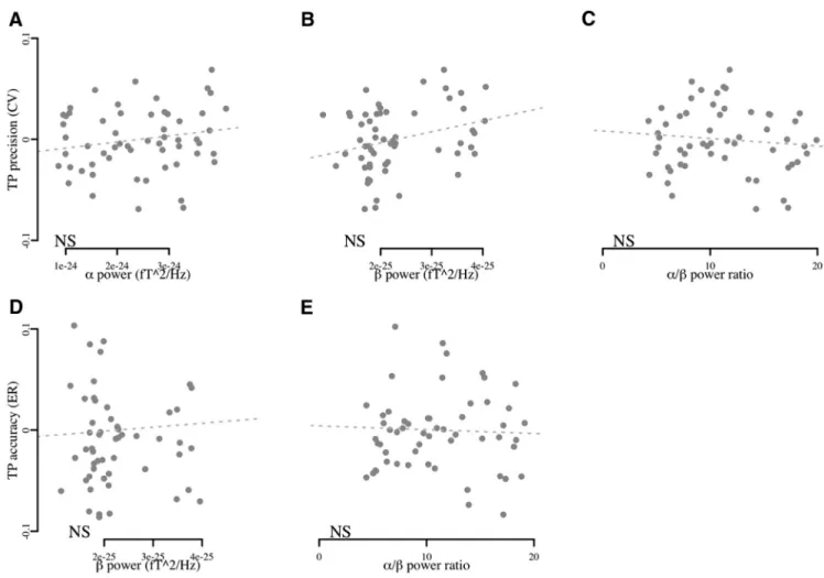
Figure 10. ␣Andpowerdonotindependentlycontributetotheprecisionintemporalperformance.Overallblocksandparticipants,theCVsoftimeintervaldidnotsignificantlycorrelatewith
the strength of␣ or  power or their ratio (A–C, respectively). In the absence of significant contributions of ␣ or  power to ER in TP (D, E, respectively), TP did not correlate with the strength of  power or ␣– power ratio. This set of results further strengthens the finding that it is the coupling of ␣–, and not ␣ or  alone that contribute to temporal precision.
Figure 11. ␣– PAC index performance accuracy. A decrease in ER of time production was
near significantly correlated with a decrease in␣– coupling strength. The shaded area around the regression line indicated standard error.
performance (
Fig. 9
). These results suggest that
␣– coupling
indexes the precision with which information may be
endoge-nously maintained, and transferred, within brain networks
dur-ing an endogenous cognitive task.
␣– PAC is not related to motor preparation or learning
Accounting for the present findings with existing evidence for the
implication of PAC in motor preparation and learning would be
tempting but several results suggest that this may not be the case
here. First, none of the frequency regimes in our study conformed
to previous reports: for instance, in intracranial recordings and
electrocorticography, motor preparation induced coupling in
␣-high ␥ with an enhanced coupling during the preparation
compared with the movement execution (
Yanagisawa et al.,
2012
;
Combrisson et al., 2017
). Additionally,
␦–␣ PAC
contralat-eral to the side of the motor preparation was found to increase
during movement versus no movement (
Kajihara et al., 2015
). In
situations of aberrant oscillatory regimes, such as in patients with
Parkinson,
de Hemptine et al. (2015)
described an increased
-high ␥ PAC. Although we cannot be fully exhaustive, motor
functions have typically been linked to other frequency coupling
than the
␣– PAC observed here.
Another line of research reported the enhancement of PAC
during learning (
Tort et al., 2009
), understood as a progressive
improvement in the measured neural or behavioral feature over
the course of the experiment (
Tort et al., 2009
;
Kononowicz and
Van Rijn, 2011
). In our study, participants’ behavioral precision
was stable over experimental blocks, suggesting no effect of
prac-tice or learning in the course of the experiment. Additionally, the
association between the strength of
␣– PAC with behavioral
precision was stable over blocks. It would thus be presently
diffi-cult to interpret our results in the context of learning (
Tort et al.,
2009
). Although different durations may entail different working
memory loads, we also did not find any increase in the strength of
PAC with the length of duration. As our experimental design did
not explicitly manipulate learning or memory during time
pro-duction, we cannot fully conclude on their possible interactions
with the reported effect and these aspects would be helpful to
manipulate in future work.
Maintenance of an endogenous temporal goal through
␣– coupling
The specific role of
␣ oscillations in cognition and information
processing remains largely debated (
Roux and Uhlhaas, 2014
)
but several observations show some consistencies. Among them,
␣ oscillations have seminally been associated with the inhibition
of irrelevant information (
Klimesch et al., 2007
;
Jensen and
Mazaheri, 2010
;
Haegens et al., 2012
) and the maintenance of
contents in working memory (
Bonnefond and Jensen, 2012
). The
power of
␣ oscillations has been shown to increase during
cogni-tive tasks requiring internal engagement, which supports the
protective role of
␣ rhythms against exogenous distraction
(
Scheeringa et al., 2009
).
␣ Oscillations have also been shown to
play an active role in working memory maintenance (
Palva and
Palva, 2011
) and in anticipation (
Haegens et al., 2012
;
Praamstra
et al., 2006
). Both anticipation (
Fortin and Masse´, 2000
;
Fortin et
al., 2005
;
Coull et al., 2013
) and maintenance of task goal (
Lustig
and Meck, 2001
) are vital functions in time estimation. Hence,
Figure 12. The strength of␣– oscillatory coupling regulates timing precision. An individual’s precision in a TP task may depend on the strength of ␣– PAC. Higher precision corresponds to a narrower distribution of temporal productions (top left; behavioral data for individual S09), whereas a lower precision corresponds to a broader distribution of temporal productions (bottom left, behavioral data for individual S02). Right, Time-frequency plots of the mean power time-locked to the phase of ␣ (here, the peak). For one individual with high behavioral precision (S09; top), a strong␣– PAC can be seen. The peak count distribution of  power maxima relative to the ␣ phase that are provided on the right shows, for individual S09, a strong concentration of maximal  power with the ␣ phase. Conversely, for the individual with lower behavioral precision (S02; bottom), a weaker ␣– PAC was found: the peak count distribution of  power maxima relative to the␣ phase for this individual showed a flatter distribution indicated a lower dependency of  power maxima on ␣ phase.