TH `
ESE
En vue de l’obtention du
DOCTORAT DE L’UNIVERSIT´
E DE TOULOUSE
D´elivr´e par : l’Universit´e Toulouse 3 Paul Sabatier (UT3 Paul Sabatier)
Pr´esent´ee et soutenue le 15/01/2015 par :
Thi Hong Hiep NGUYEN
Strong consistencies for Weighted Constraint Satisfaction Problems
JURY
MARTIN COOPER Professeur d’Universit´e Pr´esident du Jury SAMIR LOUDNI Maˆıtre de conf´erences Membre du Jury CHRISTOPHE LECOUTRE Professeur d’Universit´e Membre du Jury PHILIPPE J ´EGOU Professeur d’Universit´e Membre du Jury CHRISTIAN BESSI `ERE Directeur de Recherche Membre du Jury THOMAS SCHIEX Directeur de Recherche Membre du Jury
´
Ecole doctorale et sp´ecialit´e :
MITT : Domaine STIC : Intelligence Artificielle
Unit´e de Recherche :
Institut National de la Recherche Agronomique (UR 0875)
Directeur(s) de Th`ese :
Thomas SCHIEX et Christian BESSI `ERE
Rapporteurs :
En premier lieu, je tiens à exprimer ma plus profonde gratitude à mon directeur de thèse Thomas Schiex pour avoir assuré la direction scientifique de ce travail de recherche, pour la confiance qu’il m’a accordé et pour son soutien déterminant tout au long de ces presque quatre années. Ses conseils judicieux et ses encouragements m’ont aidée à surmonter les difficultés au travail ainsi que dans la vie pour aller jusqu’au bout de cette thèse.
Toute ma reconnaissance va également à mon Co-directeur de thèse, Christian Bessière, pour sa direction scientifique, ses commentaires pertinents et ses précieuses corrections. Je suis consciente d’avoir eu la chance de travailler avec lui.
Ma reconnaissance s’adresse aussi à Simon de Givry pour son soutien technique qui m’a per-mis d’avancer de manière efficace dans mon travail d’implémentation et d’expérimentation. Je tiens à remercier Mickaël qui m’a aidée à régler des problèmes informatiques sur mon ordinateur.
Mes plus sincères remerciements vont également à l’ensemble des personnes qui m’ont fait l’honneur de juger ce travail : à Martin Cooper pour avoir accepté de présider le jury, à Christophe Lecoutre et Phillipe Jégou pour leurs commentaires avisés en tant que rapporteurs, et enfin, à Samir Loudi pour ses remarques précises lors de ma soutenance. Je remercie les collègues qui ont été à mes côtés plus ou moins longtemps durant cette période de ma vie et avec lesquels je partage de nombreux souvenirs. Magali, mon dieu, merci pour ton aide administrative et tes indications sur le travail de thèse. Un grand merci à ma fillette Charlotte pour ta bonne humeur et ton encouragement qui m’ont aidée à trouver l’équilibre dans la vie et la motivation au travail lorsque j’ai rencontré des dif-ficultés personnelles. Je tiens à remercier Julia et Anaïs pour les bons moments qu’on a partagés et pour les soirées au bord de la Garonne que je n’oublierai jamais. Je voudrais remercier Mahuna et Aurélie pour leur gentillesse et leur sympathie ; grâce à eux, j’ai pu me rapprocher de la bande des non-permanents.
Je tiens à remercier tous les membres, stagiaires, chercheurs, techniciens et secrétaires de l’unité MIAT du laboratoire INRA pour leur gentillesse et sympathie. Merci a Fabienne Ayrignac pour m’avoir accueillie au sein du labo et pour m’avoir aidée pendant mes premiers jours en France. Un grand merci à David Allouche pour les temps d’échange qu’on a partagés, en particulier nos discussions sur la vie, et pour les grands moments à Noël que j’ai passé avec ta famille.
Je remercie mes amis vietnamiens à Toulouse et au Vietnam pour leur soutien et leur aide: Chien, Bai, Hanh, Luyen, Ly, Diep, Thao, Thu, Trung, Lam, Hoai, Bao Anh, Phuong, Binh .... Grâce à eux, ces quatres années sont passées plus vite. Un grand merci à Chien
Enfin, j’exprime ma gratitude à ma famille pour leurs encouragements et leur amour infini. Cảm ơn bố mẹ đã sinh ra con, luôn động viên và dõi bước trên đường đời của con. Khi vui cũng như buồn, thành công hay thất bại, bố mẹ luôn bên con và nâng đỡ cho con. Tình yêu ấy là động lực để con vượt qua mọi sóng gió cuộc đời và gặt hái nhiều thành công.
1 Introduction 1
1.1 Thesis’s motivation. . . 1
1.2 Thesis’s organization and contributions. . . 3
2 Background 5 2.1 Constraint satisfaction and hard consistencies . . . 5
2.1.1 Constraint satisfaction problems . . . 5
2.1.2 Backtracking search . . . 6
2.1.3 Constraint propagation . . . 6
2.1.4 Arc consistency . . . 7
2.1.5 Arc consistency algorithms. . . 8
2.1.6 Restricted arc consistencies . . . 10
2.1.7 Strong consistencies . . . 10
2.1.8 Comparison between consistencies . . . 16
2.1.9 Revision ordering heuristics . . . 17
2.1.10 Dynamic arc consistency . . . 18
2.2 Weighted CSP and soft consistencies . . . 20
2.2.1 Weighted constraint satisfaction problems. . . 22
2.2.2 Branch-and-Bound search . . . 22
2.2.3 Equivalent Preserving Transformations . . . 23
2.2.4 Soft consistencies . . . 25
2.2.5 Soft arc consistencies . . . 26
2.2.6 High order consistencies . . . 33
2.2.7 Virtual arc consistency . . . 37
3 Dynamic virtual arc consistency 43 3.1 Introduction . . . 43
3.2 Maintaining VAC dynamically during successive iterations . . . 44
3.2.1 Specification of changes in Bool(P) . . . 44
3.2.2 Algorithm. . . 46
3.2.3 Example. . . 47
3.2.4 Correctness of the algorithm. . . 49
3.2.5 Complexity . . . 50
3.3 Maintaining VAC dynamically during search . . . 50
3.3.1 Specification of changes in Bool(P) . . . 50
3.3.2 Algorithm. . . 53
3.3.3 Example. . . 54
3.4 Experimentation . . . 56
3.4.1 VAC implementation . . . 56
3.4.2 Set of benchmarks . . . 57
3.4.3 Experimental results . . . 58
3.5 Conclusions . . . 61
4 Soft high order consistencies 63 4.1 Introduction . . . 63
4.2 Definitions of soft high order consistencies . . . 64
4.2.1 Soft restricted path consistencies . . . 66
4.2.2 Soft path inverse consistencies. . . 68
4.2.3 Soft max-restricted path consistencies . . . 69
4.3 Comparison between soft domain consistencies . . . 71
4.3.1 Stronger relation . . . 71
4.3.2 Relation graph . . . 73
4.4 Enforcing algorithms. . . 82
4.4.1 Equivalence Preserving Tranformations . . . 82
4.4.2 Enforcing soft path inverse consistencies. . . 84
4.4.3 Enforcing soft max-restricted path consistencies . . . 94
4.5 Experimentation . . . 104
4.5.1 Benchmarks and experiments . . . 104
4.5.2 Pre-processing by PICs and maxRPCs. . . 105
4.5.3 Pre-processing by a restricted version of PICs and maxRPCs . . . 116
4.5.4 Maintaining PICsr and maxRPCr during search . . . 119
4.5.5 Conclusion . . . 128
4.6 Conclusions . . . 128
5 Conclusions and perspectives 129 5.1 Dynamic Virtual Arc Consistency . . . 129
5.1.1 Conclusions . . . 129
5.1.2 Perspectives . . . 130
5.2 Soft high order consistencies . . . 130
5.2.1 Conclusions . . . 130
Introduction
1.1
Thesis’s motivation
A wide variety of real-world optimization problems can be modeled as weighted constraint satisfaction problems (WCSPs). A WCSP or a cost function network (CFN) consists of a set of variables and a set of cost functions where the costs are associated to assignments to the variables, expressing preferences between solutions. The goal is to find an assignment to the variables which minimizes the combined costs. This kind of problem has applications in resource allocation [Cabon et al., 1999], combinatorial auctions, bioinformatics [Traoré et al.,2013]. . .
WCSPs, as many optimization problems, can be solved by Depth First Branch-and-Bound Search. This method allows to keep a reasonable space complexity but requires good (strong and cheap) lower-bounds on the minimum cost of a node to be efficient. The quality of lower-bounds should be put into balance with their computational time in order to accelerate the search.
In the last years, increasingly better lower-bounds have been designed by enforcing soft con-sistencies in WCSPs. Soft concon-sistencies aim at simplifying WCSPs by defining properties on the cost of values or assignments of values that must be satisfied. Soft consistencies are enforced by iteratively applying so-called Equivalence Preserving Transformations (EPTs, [Cooper and Schiex,2004]). EPTs extend the traditional local consistency operations used in classical CSPs by moving costs between cost functions of different arities while keeping the problem equivalent. By ultimately moving cost to a constant function with empty scope, they are able to provide a lower-bound on the optimum cost which can be incre-mentally maintained during Branch-and-Bound search.
Among the proposed soft consistencies for WCSPs, soft arc consistencies such as AC*, DAC*, FDAC* or EDAC* [Larrosa et al.,2005], extended from the classical AC used in classical CSPs, require a small enforcing time but do not always provide tight lower-bounds that lead to massive pruning. They are enforced by applying, in an arbitrary order, specific EPTs, called Soft Arc Consistency (SAC) operations, which shift costs between values and cost functions of arity either greater than 1 or equal to 0 (defining the lower-bound). Optimal Soft Arc Consistency (OSAC) can provide optimal lower-bounds (in the sense that applying any sequence of SAC operations cannot result in a better lower-bound) but is too expensive for general use. Instead, Virtual Arc Consistency (VAC [Cooper et al.,
2008,2010]) is cheaper than OSAC while providing lower-bounds stronger than other soft arc consistencies.This is obtained by using a planned sequence of SAC operations defined from the result of enforcing classical AC on a classical constraint network which forbids combinations of values with non zero costs.
Beyond arc consistencies, up to now, only few high order consistencies have been pro-posed for WCSPs such as complete k-consistency [Cooper, 2005] extended from hard k-consistency, Tuple Consistency [Dehani et al., 2013] considered soft arc consistencies applied to tuples (combinations of values) instead of values, . . .
Indeed, this thesis is motivated by two questions. First, is it possible to improve the efficiency of enforcing for existing soft consistencies? Second, can we propose new soft consistencies for WCSPs that provide strong lower-bounds but have a reasonable time complexity?
We realized that VAC can be accelerated by exploiting its iterative behavior. Indeed, each iteration of VAC requires to enforce classical AC on the hardened version of the current network. But this network is just the result of the incremental modifications done by EPTs applied in the previous iterations. Similarly, maintaining VAC during search requires to enforce classical AC on the hardened version of the current network which are slightly modified due to branch operations. This situation, where AC is repeatedly enforced on incrementally modified versions of a constraint network, has been previously considered in Dynamic Arc Consistency algorithms [Barták and Surynek, 2005; Bessière, 1991] for Dynamic CSPs [Dechter and Dechter,1988]. Thus, integrating Dynamic Arc Consistency into VAC is a potential approach for improving the enforcing time of VAC by inheriting the work done in previous iterations of VAC or in parent nodes.
Soft consistencies can be extended from hard consistencies by replacing the notion of com-patibility in classical CSPs by the notion of zero-cost in WCSPs. For example, hard arc consistency in binary CSPs requires that any value of any variable has a compatible value, called an (hard) arc support, in every adjacent domain. Soft arc consistencies redefine this feature by replacing the compatibility of the supporting values by the requirement of zero-cost between values and their supporting values.
Based on this principle, we can create strong consistencies for WCSPs by extending (hard) high order consistencies (HOCs). Among hard HOCs, we are interested in the group of triangle-based consistencies consisting of RPC, PIC, maxRPC because of two reasons: (1) these are domain-based consistencies; (2) they have a strong pruning power while having a reasonable time complexity. Thus, extending these potential hard consistencies to WCSPs would lead to strong soft consistencies, as desired.
In summary, the objective of this thesis is to focus on soft consistencies for efficiently solving WCSPs. We would like to improve the enforcing time of VAC by using Dynamic Arc Consistency for maintaining classical Arc Consistency in the hardened version of WCSPs. In addition, we would like to investigate soft high order consistencies by extending hard triangle-based consistencies to WCSPs in order to provide strong lower-bounds for Branch-and-Bound search.
1.2
Thesis’s organization and contributions
OrganizationThis thesis consists of three chapters. A background survey in the domain of (Weighted) Constraint Satisfaction Problems is introduced in the first chapter while the thesis contri-butions are presented in the two last chapters.
Chapter 2 outlines in the first section background knowledge on classical CSPs and hard consistencies. Then, it reviews Weighted CSPs, operations of shifting costs, basic soft consistencies and algorithms enforcing them.
In Chapter3, we propose Dynamic Virtual Arc Consistency, an improved version of Virtual Arc Consistency for WCSPs. An enforcing algorithm and the properties of the algorithm are also discussed in this chapter.
In the last chapter, we propose soft high order consistencies extended from hard RPC, PIC and maxRPC. A general comparison on the performance of soft domain-based consistencies is also proposed in this chapter. The enforcing algrorithms and experimental results of soft high order consistencies will be presented.
Contributions
This thesis has two main contributions for efficiently solving WCSPs: improving the ef-ficiency of enforcing VAC and proposing high order consistencies. An outline of these contributions is presented below.
Dynamic virtual arc consistency
By integrating Dynamic Arc Consistency inside VAC algorithm to maintain hard Arc Consistency in the hardened version of WCSPs P , called Bool(P), we can dynamically maintain VAC during iterations of VAC and during search. This new algorithm is named Dynamic Virtual Arc Consistency (DynVAC). We have proposed two variants of DynVAC, called normal and full DynVAC when maintained during search.
• Normal DynVAC maintains arc consistency in Bool(P) inside each search node, i.e. during iterations of VAC, and rebuilds Bool(P) from scratch when the search branches out.
• Full DynVAC maintains arc consistency in Bool(P) both inside nodes and during search.
We have given an implementation for two variants of DynVAC in the solver toulbar2. Domain-based revision order heuristics are also implemented inside each variant of Dyn-VAC.
Soft high order consistencies
We have proposed 18 soft high order consistencies extended from hard RPC, PIC, and maxRPC, with six variants for each one. The six soft consistencies based on hard RPC are simple RPC, directional RPC, full directional RPC, existential RPC, existential directional RPC and virtual RPC. This is the same for the cases of hard PIC and hard maxRPC. Two “stronger” relations for comparing soft domain-based consistencies have also been proposed in this thesis. Based on these relations, we have given a general comparison of our soft high order consistencies and soft arc consistencies.
We have designed algorithms for enforcing soft high order consistencies extended from hard PIC and maxRPC. These algorithms have been characterized in terms of termination, time and space complexities.
Finally, an implementation of soft RPCs and soft maxRPCs in toulbar2 has been done and experimental results are presented. The impact of our consistencies on the search has also been analyzed.
Background
2.1
Constraint satisfaction and hard consistencies
2.1.1 Constraint satisfaction problemsDefinition 2.1 (Constraint satisfaction problem) A constraint satisfaction problem (CSP) or constraint network (CN) is a tuple P = (X, D, C). X is a finite set of variables. Each variable xi∈ X has a finite domain D(xi) ∈ D. C is a finite set of constraints. Each
constraint cS ∈ C is a relation defined on a subset of variables S ⊆ X that specifies the
allowed combinations of values for variables on S. S and ∣S∣ are called the scope and the arity of the constraint.
Many academic and real problems can be formulated as CSPs. For example, the N-queens problem can be modeled as a CSP with N variables X = (x1, . . . , xN) where xi is defined
for the queen placed in the column i. The value of xi represents its line number and the
domain of xiis a set of integers D(xi) = {1..N}. The constraints on non-sharing of lines and
diagonals by 2 queens xi and xj are respectively represented as xi ≠ xj and∣xi−xj∣ ≠ ∣i−j∣.
Definition 2.2 (Normalized CSP) A CSP is normalized iff there does not exist any two constraints defined on the same scope.
A constraint defined over a scope of k variable is called k-ary. The notation ci and cij
denote the unary and binary constraint on variable xi and on variables xi, xj respectively.
A binary CSP has only unary and binary constraints and a non-binary CSP has also non-binary constraints.
Definition 2.3 (Instantiation and Solution) Given a CSP P = (X, D, C).
• An instantiation τSon a set of variables S⊆ X is an assignment of values for variables
in S: τS∈ `(S). S is called the scope of τ.
• τS is a partial instantiation if S⊂ X or a complete instantiation if S = X.
• An instantiation τS is locally consistent if it satisfies all constraints cT such that
T ⊆ S.
• A solution of the CSP is a complete instantiation which is locally consistent. The set of solutions of P is denoted by sol(P).
• An instantiation τS is globally consistent if it is locally consistent and can be extended
to a solution.
An instantiation is also called a tuple. For a tuple τS, a variable x∈ S and a subset W ⊂ S,
τ[x] and τ[W] denote respectively the value of x in τS and the projection of τS on W
which is the set of values assigned by τS for the variables of W . For a constraint cS and a
tuple τS, we denote by τS ∈ cS the fact that τS is an allowed instantiation of cS and τS/∈ cS
the fact that τS is forbidden. When the variable x is assigned to a value a ∈ D(x), this
is denoted by (x, a) or xa. For a given CSP, the notations n, d, e respectively denote the
number of variables, the maximum domain size and the number of constraints of the CSP. The task of a CSP is to find a complete instantiation of values which satisfies all the constraints of the problem. If there does not exists any such solution, the problem is unsatisfiable, inconsistent or unfeasible. Otherwise, the problem is satisfiable, consistent or feasible. Deciding consistency is a NP-complete problem.
There are three main approaches for solving constraint satisfaction problems: backtrack-ing search [van Beek, 2006], local search [Hoos and Tsang,2006], and dynamic program-ming [Dechter,2006]. Backtracking search as well as the technique “constraint propagation” for improving its efficiency will be recalled in this thesis.
2.1.2 Backtracking search
Backtracking search [Golomb and Baumert,1965] is the simplest method for solving CSP problems that was first proposed by. It is a modified depth-first search of a tree. The idea is to search in a tree of variable assignments in which each intermediate node is a partial variable assignment and each leaf is a complete variable assignment. As we move down in the tree, we may assign (or restrict the domain of) a variable and a new node is created. Then, the partial variable assignment of that node will be checked for local consistency to determine whether the node can be extended to a solution or not. If the node cannot lead to a solution, it is a dead-end and the search backtracks to the parent node. Otherwise, an unassigned variable will be chosen to be assigned or restricted and the search will continue at the deeper level. A leaf satisfying all the constraints is a solution of the problem. In the literature, there exists many backtracking search algorithms that are distinguished by the way constraints at a node are checked and by the way the search backtracks. For example, the naive backtracking search only checks constraints with no unassigned variable at a node while the forward checking algorithm [McGregor,1979;Haralick and Elliot,1980] only checks constraints with one assigned variable and one unassigned variable. In the naive backtracking search, the root of the search tree is an empty variable assignment. The partial assignment on the path to each node is checked to determine whether it is locally consistent or not. If a constraint check fails, the search stops its depth moves and the next value in the domain will be assigned to the current variable. If no value is left, the search will backtrack up to the most recently assigned variable.
2.1.3 Constraint propagation
Constraint propagation is a technique for improving the efficiency of backtracking search. It focuses on search space reduction by early elimination of locally inconsistent instantiations.
The idea is to maintain a necessary property, called a local consistency, that values or instantiations of values need to satisfy to belong to solutions. It requires for each scope S of a given size that each locally consistent instantiation τScan be extended to an instantiation
τS′ on a larger scope: S⊂ S′ and τS′[S] = τS. The simplest consistency for CSPs is node
consistency which requires that each domain value must satisfy all unary constraints defined for the variable.
Definition 2.4 (Node consistency) A variable x is node consistent iff for every value v ∈ D(x), for every unary constraint cx, v ∈ cx. A CSP is node consistent if every of its
variables is node consistent.
For a local consistency, a value (or instantiation) is said to be locally consistent if it satisfies the given local consistency and is called locally inconsistent otherwise. The locally inconsistent values (instantiations) cannot belong to any solution of the problem. They can therefore be removed from the problem without removing solutions. A problem is called locally consistent w.r.t a local consistency property if all its values (or instantiations) are locally consistent. Local consistencies are grouped in two classes: “domain-based” for the ones which define conditions on values and “constraint-based” for those which define conditions on instantiations of arity higher or equal to 2.
Every local consistency can be enforced by a transformation, called constraint propagation or filtering, which iteratively removes locally inconsistent values (instantiations) until no such value (instantiation) exists. This transformation changes the problem while preserving its equivalence in terms of the set of solutions. The strength of constraint propagation comes from the fact that the removal of locally inconsistent values (instantiations) can make other values (instantiations) no longer able to locally satisfy the related constraints, and thus also locally inconsistent.
The final result of constraint propagation for a consistency Φ on a CSP P is called the Φ−closure of P, denoted as Φ(P). The Φ−closure of P is a problem which satisfies the property Φ and which is equivalent to P (having the same set of solutions). The Φ−closure is unique for a given P if Φ is a domain-based property stable under the union operation in the sense that the union of two problems Φ−consistent defined on the same set of variables and constraints is also Φ−consistent: (X, D1, C) ∪ (X, D2, C) = (X, D1∪ D2, C) [Bessiere,
2006].
2.1.4 Arc consistency
Every CSP can be viewed as a network of constraints, where each variable is represented by a node and each binary (non binary) constraint is represented by an arc/edge (hyper arc/edge). Arc consistency defines the consistency of arcs in such a way that for a constraint and an involved variable, every value of the variable can be extensible to a consistent instantiation of the variables of the (hyper)-arc.
Definition 2.5 (Arc consistency) A constraint cS is arc consistent iff for every variable x ∈ S and every value v ∈ D(x), there exists a tuple τS such that τS[x] = v and τS ∈ cS.
Such a tuple is called a support for the value (x, v) on c. A CSP is arc consistent iff all its constraints are arc consistent.
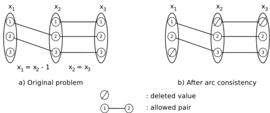
Example 2.1 Consider the binary CSP in Figure 2.1(a). It has 3 variables x1, x2, x3
Figure 2.1: Enforcing arc consistency
x2− 1), (x2= x3). Each value is represented by a vertex. An arc between two values means
that the corresponding pair of values are authorized. Checking constraint c12 detects the
arc inconsistent value 3 in D(x1) because there is no value in D(x2) compatible with it. In
other words, there is no support in D(x2) for (x1, 3) and this value will be removed. Value
(x2, 1) also can be removed because of c12. The removal of value(x2, 1) makes value (x3, 1)
arc inconsistent and (x3, 1) will be removed. Now, every remaining value has a support on
every constraint, and the resulting problem is arc consistent (Figure 2.1(b)).
Arc consistency is also called generalized arc consistency (GAC) in many documents when the authors want to emphasise the fact that AC is used on non-binary CSPs. In this case, AC is specialized for binary CSPs.
An arc consistent CSP is not necessarily satisfiable. The coloring problem in Figure 2.2 is an example. It has 3 variables with 2 colors for each one and 3 constraints c12(x1 ≠
x2), c23(x2 ≠ x3), c13(x1 ≠ x3). This problem is arc consistent but it is unsatisfiable since
it is impossible to color a 3-clique with 2 colors only.
Figure 2.2: Example of an unsatisfiable CSP which is AC
2.1.5 Arc consistency algorithms
Many algorithms have been proposed for enforcing AC in order to improve the efficiency of enforcing. Bessiere gives two important reasons for studying AC algorithms in [Bessiere,
2006]: AC is the basic mechanism used in all solvers and each technique to improve AC can be applied for other consistency algorithms. AC enforcing algorithms are grouped in 2 classes: coarse-grained and fine-grained, where the former ones propagate the changes in the variable domains while the second ones propagate the value removals.
AC3
AC3 is one of the first efficient algorithms for enforcing arc consistency, proposed by Mack-worth[1977]. As a coarse-grained algorithm, it propagates changes in the domain of vari-ables to neighbor varivari-ables by using a propagation list that contains arcs, varivari-ables, or constraints related to the reduced domains.
There are three variants for AC3 implementation: arc-oriented [Mackworth,1977], variable-oriented [McGregor, 1979] and constraint-oriented [Boussemart et al., 2004a] In the first variant, the propagation list contains arcs where each arc is composed of a constraint and a variable involved in the constraint that needs to be revised. The second variant stores in the propagation list the variables with reduced domains and the last one stores the constraints involving at least a variable to be revised.
AC3 does not store any additional information, thus it can make many unnecessary con-straint checks. Precisely, when revising a variable in a concon-straint, it has to check all values of the variable regardless of whether these values have lost their support or not. In binary CSPs, AC3 has a complexity in O(ed3) in time and O(e) in space where e is the number
of constraints and d is the maximum domain size. AC4
In order to improve AC3, Mohr and Henderson [1986] proposed the AC4 algorithm that memorizes a maximum amount of information. It maintains the number of supports for each value on each constraint in a counter. Whenever the counter of a value decreases to 0, the value will be removed and the counters of all its neighbor values will be decreased by 1. Thanks to the counter system, no constraint check is performed during the run of AC4 algorithm. Constraints are only checked once at start-up. Furthermore, AC4 stores the list of values supported by each value. When a value is removed, only values that have been supported by the removed value need to be verified. This list allows AC4 to avoid considering unnecessary values which have not been supported by the removed values. Compared to AC3, AC4 has a better time complexity in O(ed2) but needs more space in
O(ed2).
AC6
AC4 spends a lot of time to compute and update the “counters” as well as the lists of supported values whereas the search for all supports is not necessary for consistent values. Therefore,Bessière[1994] proposed AC6 in order to avoid such unnecessary computation of AC4. Instead of keeping the complete support sets and counters, AC6 remembers only one support for each value. AC6 cancels the “counter” information and stores for each value the list of values that are currently supported by it. When a value is removed, AC6 will search for a new support for the values that were supported by the removed value. Thanks to the order of values in domains, the search for a new support always starts from the current support to the end of the domain, until the next support is found. All the values before the current support of the considered value were verified as incompatible with it. Thus, AC6 can avoid redoing constraint checks despite of the unknown number of supports. AC6 has the same time complexity in O(ed2) as AC4 but it reduces the space complexity to O(ed).
AC2001 & AC3.1
Both AC4 and AC6 are fine-grained algorithms. The disadvantage of these algorithms is that the value-oriented propagation queue is expensive to maintain. Therefore, Bessière and Régin[2001] proposed a coarse-grain algorithm AC-2001 which keeps the optimal time complexity of AC6, by memorizing only the current support for each value in order to avoid redundant constraint checks. This idea is also used in [Zhang,2001] in an algorithm named AC3.1. AC2001 uses a pointer to store the first support for every value on each constraint. On the one hand, this data structure is easier to implement and maintain than the lists of supported values used in AC6. On the other hand, similarly to the lists of supported values used in AC6, it allows AC2001 to stop the search for supports as soon as possible. The search for a new support for a value on a constraint does not check again values before the current support which were previously proved as incompatible with the considered value. In spite of the fact that AC2011 has the same asymptotic time and space complexity as AC6, it can provide speed-ups in practical experiments because of its simplicity.
2.1.6 Restricted arc consistencies
In order to reduce the computational cost of arc consistency when being maintained during the backtracking search, many domain-based consistencies which are weaker than AC in terms of pruning power but have a cheaper computational cost have been proposed. The usual idea of these consistencies is to weaken AC by reducing the work AC does, i.e., reducing either the number of calls to constraint checks or the amount of work inside each constraint check. The former checks AC for only some of constraints while the last checks AC for some of domain values (e.g.; the minimum and the maximum values of domains in the case of consistencies on bound). In summary, these restricted consistencies of AC enforce arc consistency in an incomplete way by skipping some values or some constraints. Directional arc consistency
Directional arc consistency (DAC [Dechter and Pearl,1988]) tries to reduce the number of constraint checks by defining an order “<” among variables and enforcing AC only on arcs directed along this order. A variable i is directed arc consistent iff it is arc consistent for all constraints cij such that i< j. A variable must be consistent with all variables greater than
it, regardless of smaller ones. Thus, each variable needs to be checked for arc consistency with respect to greater variables and the removal of a value from the domain of a variable cannot make greater variables directed arc inconsistent. Thanks to this property, DAC does not need to use a propagation queue, just a loop processing variables w.r.t the DAC order from the greatest to the smallest one.
2.1.7 Strong consistencies Path consistency
Path consistency, proposed byMontanari[1974], is the most studied constraint-based local consistency. In binary CSPs, path consistency is simply an extension of arc consistency
which consists in extending the pairs of variables, instead of singleton variables, on every other variable. A pair of variables is path-consistent with respect to a third variable iff for every consistent pair of values, there exists a value of the third variable compatible with this pair in such a way that the 3-values tuple satisfies all the binary constraints.
Definition 2.6 (Path consistency (PC)) A CSP is path consistent iff for every pair of variables (xi, xj), for every consistent pair of values (vi, vj) ∈ D(xi) × D(xj), for every
third variable xk connected with xi, xj by cik, cjk, there exists a value vk∈ D(xk) such that
(vi, vk) ∈ cik and (vj, vk) ∈ cjk.
Many algorithms have been proposed to enforce path consistency, that differ each other by the data structures and by the enforcing efficiency. The first one, PC−1, is a naive algorithm that has time complexity in O(n5d5) [Montanari, 1974]. PC−2 [Mackworth, 1977] and
PC−3 [Mohr and Henderson, 1986] respectively improve this complexity to O(n3d5) and
O(n3d3) by using the idea of AC3 and AC4 to reduce the number a triple of variables is checked. However, Han and Lee[1988] proved that PC−3 is not correct. When a pair of values has no compatible value on a third variable, PC−3 remove the two values of the pair instead of forbidding the pair. Thus, they proposed a correct version, PC−4, that has a same complexity O(n3d3) in time and space. Then, PC−5 [Singh, 1995] and
PC−6 [Chmeiss,1996] were independently proposed to improve the average time complexity of PC−4 to O(n3d2) by basing on AC6 instead of AC4. PC−7 [Assef Chmeiss,1996] has a
smaller time complexity in O(n2d2).
k−consistency
Based on the idea of node and arc consistencies which respectively consist in consis-tently extending zero and one variable on every another one, [Freuder, 1978] introduced k−consistency for consistently extending k − 1 variables to every extra one. It guarantees that for each consistent instantiation of k− 1 variables, there exists a value for every k−th variable such that the k−values instantiation satisfies all constraints among them.
Definition 2.7 (k-consistency) A CSP is k-consistent iff for every set of k−1 variables Y, for every consistent instantiation τY, for every k-th variable xk, there exists a value
vk∈ D(xk) such that τY ∪ (xk, vk) is consistent. The CSP is strongly k-consistent iff it is
j-consistent for every j≤ k.
Figure 2.3: A 4-inconsistent CSP
Example 2.2 Consider the CSP in Figure 2.3. It has 4 variables with 2 values for each one, 3 binary constraints (x1 = x2), (x2 = x3), (x1 = x3) and a 4-ary constraint
c1234(x1, x2, x3, x4) = {(1, 2, 1, 1), (2, 1, 2, 2}. Allowed pairs of values for binary constraints
are represented by continuous black lines, while allowed tuples for the four-ary constraint are represented by dashed lines. Each allowed tuple uses a different color. This problem is 3-consistency but is not 4-consistency because the locally consistent instantiations (1, 1, 1) and (2, 2, 2, ) on (x1, x2, x3) cannot be consistently extended to x4.
For normalized binary CSPs (where there is are two constraints with the same scope), NC, AC and PC respectively correspond to 1,2,3-consistency. If we enforce all NC, AC, PC, we will obtain the level of strong 3-consistency. In non-binary CSPs, PC is not equivalent to 3-consistency because 3-consistency considers ternary constraints whereas PC does not. In non-normalized CSPs, AC is not equivalent to 2-consistency because there exists cases in which 2 variables are connected by more than 2 binary constraints, each one is AC but no pair of values satisfies all constraints.
Restricted path consistency
Restricted path consistency (RPC), proposed byBerlandier[1995], is half-way between AC and PC. It removes more inconsistent values than AC while avoiding some disadvantages of PC. PC checks the consistency of all pairs of values, even those of two independent variables, on any third variable. This is very expensive and can create new constraints. Thus, RPC checks only pairs of values which, if they are removed, will make a value arc inconsistent. So in addition to AC, RPC checks path consistency for pairs of values which define the unique support for an involved value. If such a unique support is inconsistent, it could be removed and this potential removal leads to the removal of the previously supported value.
Definition 2.8 (Restricted path consistency - RPC) A binary CSP is restricted path consistent iff it is AC and for all xi, for all value vi ∈ D(xi), for all cij on which vi has
a unique support vj ∈ D(xj), for all xk linked to both xi, xj by binary constraints cik, cjk,
there exists a value vk ∈ D(xk) such that (vi, vk) ∈ cik and (vj, vk) ∈ cjk. vk is called a
witness for the support (ia, jb) of (i, a) on k.
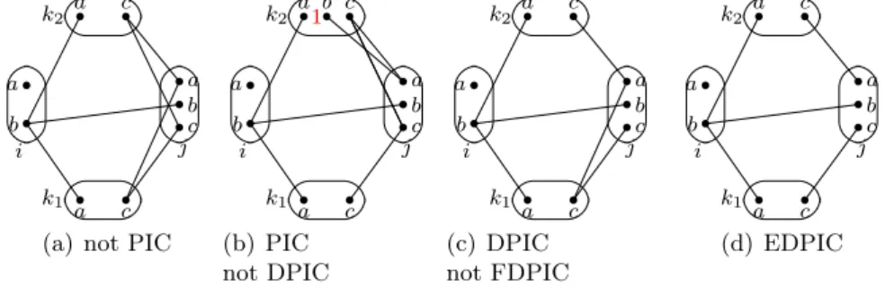
Example 2.3 Let’s consider the problem in Figure 2.4(a). Please notice that here, edges indicate forbidden pairs. It is AC but not RPC. Value (xi, 1) has only one support (1, 2)
in cij but this support cannot be extended on xk. It will be removed by RPC.
1 2 1 2 1 2 xj xk xi (a) 1 2 1 2 3 1 2 3 xj xk xi (b) 1 2 1 2 1 2 1 2 xj xl xi xk (c) forbidden pair of values
inconsistent value
Figure 2.4: Some examples for comparing AC, RPC, PIC, maxRPC [Bessiere, 2006]. a)A CSP which is AC but is not RPC. b) A CSP which is RPC but is not PIC. c) A CSP which is PIC but is not maxRPC.
RPC can prune more values than AC. In addition to the arc inconsistent values, RPC also removes the values for which their unique support is path inconsistent in some constraint. Several algorithms have been proposed for enforcing RPC. Algorithm RPC1, proposed byBerlandier[1995], is based on AC4. It also counts the number of supports for each value in each constraint, and stores the list of values supported by each value. A value needs to be checked for PC whenever its number of supports decreases to 1, and is removed whenever this number decreases to 0. RPC1 uses 2 propagation queues. The first one contains removed values, used for the AC propagation, as in AC4. The second one, used for the PC propagation, contains 3-tuples (value, constraint, triangle) for which the unique support of the value needs to be checked for PC on the triangle. RPC1 has a space complexity in O(end) and a time complexity in O(ed2) on binary CSPs.
Then,Debruyne and Bessière [1997a] proposed RPC2 which is based on the idea of AC6. RPC2 only stores the two first supports for each value in each constraint, instead of counting all supports and storing the lists of supported values as in RPC1. Whenever a value has lost supports, RPC2 will try to search next supports such that the total number of supports, including the available stored ones, does not exceed 2. RPC2 will remove a value, revise for PC or do nothing if this value has no, one or at least 2 supports respectively. Moreover, RPC2 stores current witnesses for each value on each constraint in each triangle while RPC1 does not. Thus, when checking PC, RPC2 does nothing if the current witnesses for unique supports are still available. The search for next support as well as witness is efficient because it always starts from the previous last found one. RPC2 has a time complexity in O(ed2+ cd2) and space complexity in O(ed + cd) where c is the number of triangles (clique of three binary constraints) in the problem.
Path inverse consistency
Freuder [1985] introduced k−inverse consistency in order to provide a domain-based con-sistency stronger than AC. The idea of k-inverse concon-sistency is to extend each variable to every k−1 extra variables. In fact, 2-inverse consistency (arc inverse consistency) is the same as 2-consistency (arc consistency). 3-inverse consistency (also called path inverse consistency) is the simplest inverse consistency that has a pruning power stronger than AC.
Definition 2.9 (Path inverse consistency - PIC) A binary CSP is path inverse con-sistent iff it is AC and for all xi, for all value vi∈ D(xi), for all xj, xk linked to each other
by cjk and linked both to xi by cij, cik, there exists a value vj ∈ D(xj), a value vk ∈ D(xk)
such that (vi, vj) ∈ cij,(vi, vk) ∈ cik and (vj, vk) ∈ cjk.
PIC can prune more locally inconsistent values than RPC. The problem in Figure 2.4(b) is an example: it is RPC but not PIC. Consider value(xi, 1). It is of course RPC because
it has 2 supports in every constraint cij, cik. However, none of its support in cij, cik
can be extended on xk, xj respectively. As a result, (xi, 1) cannot be extended on triple
(xi, xj, xk). Thus, this value is not PIC and will be removed by PIC.
PIC algorithms The first algorithm for enforcing PIC, called PIC1, was proposed by Freuder and Elfe [1996]. PIC1 does not use any special technique or data structure. It only uses a propagation queue containing variables which need to be checked for PIC.
When revising a variable popped up from the propagation queue, it considers every triangle involving that variable and deletes values which are not extensible on that triangle. If the domain of the revised variable has been reduced, all neighbor variables are pushed into the propagation queue. The algorithm stops when this queue is empty. The time and space complexity of PIC1 are O(en2d4) and O(n) respectively.
R.Debruyne[2000] proposed an enhanced algorithm for enforcing PIC, named PIC2, which stores additional information to avoid useless constraint checks. Firstly, PIC2 stores the list of values and the list of pairs of values currently supported by each value. When a value is removed, PIC2 only considers values and pairs of values in the lists of the removed value to check for AC and PC respectively. If no witness is found for a pair of values, PIC2 tries to search for a new PC support for the involved value by checking next pairs of values. The search for a new support and for a new witness always starts from the old one. Secondly, PIC2 uses a lexicographic order to arrange values in domains and to define an order among pairs of values. Based on AC7 [Bessiere et al.,1999], PIC2 stores the last value checked to find an AC support for each value in each constraint. Thanks to this data, each pair of values and each 3-values tuple are checked at most once for the search for supports and for witnesses respectively. The propagation queue used in PIC2 contains removed values while PIC1 store variables which needs to be checked for PC in this queue. The time and space complexity of PIC2 are O(en + ed2+ cd3) and O(ed + cd) respectively.
max-restricted path consistency
Proposed by Debruyne and Bessière [1997a], maxRPC is an extension of RPC. It checks the existence of a path consistent support for each value in each constraint, whatever the number of supports the value may have. maxRPC is an intermediate between RPC and PC. RPC and PC respectively guarantee path consistency for the unique support and for every support while maxRPC guarantees path consistency for one support of each value in each constraint. The idea of maxRPC is to remove all values which have no AC or PC support in some constraint, where a PC support is an AC support which is path consistent. For binary CSPs, a value is max-restricted path consistent if it has a PC support in every constraint.
Definition 2.10 (max-restricted path consistency) A binary constraint network is max-restricted path consistent iff it is AC and for all xi, for all value vi ∈ D(xi), for
all cij, vi has a support vj ∈ D(xj) such that for all xk linked to both xi, xj by a constraint,
there exists a value vk∈ D(xk) such that (vi, vk) ∈ cik and(vj, vk) ∈ cjk.
In the case of non-binary CSPs, maxRPC requires AC for non-binary constraints and maxRPC as defined above for binary constraints.
maxRPC prunes more values than PIC. The CSP in Figure2.4(c) is PIC but is not maxRPC due to the value(xi, 1). It has 2 AC supports on cik. The support(1, 1) on (xi, xk) can be
consistently extended on xj but cannot on xl. Conversely, the support(1, 2) on (xi, xk) can
be consistently extended on xl but cannot on xj. In summary,(xi, 1) has no AC support
that can be consistently extended on xj and xl at the same time.
maxRPC algorithms The first algorithm for enforcing maxRPC is a fine-grained one, named maxRPC1, which was proposed byDebruyne and Bessière[1997a] for binary CSPs.
It is built based on RPC2 by using the same data structures and memorizing the same information as in RPC2. maxRPC1 also stores the list of values supported by each value and the list of pairs of values witnessed by each value. The difference between RPC2 and maxRPC1 is that maxRPC1 memorizes the first PC support instead of the 2 first AC supports for each value in each constraint. When a value is removed, maxRPC1 will search for a new PC support for all values currently supported by it and search for a new witness for all pairs of values currently witnessed by it. If no witness is found for a pair of values, maxRPC1 will search for a new PC support by considering next pairs of values. maxRPC1 has a space and time complexity in O(ed + cd) and O(en + ed2+ cd3) respectively. This
time complexity is known as being optimal for enforcing maxRPC.
maxRpc2 [F. and G., 2003] is a coarse-grained maxRPC algorithm which has the same complexity as maxRPC1 but takes a smaller space complexity in O(ed). Based on AC2001, maxRPC2 uses a pointer to store the last PC support for each value in each constraint. However, maxRPC2 does not store witnesses of PC supports. Thus, maxRPC2 combines the procedure for checking PC witness loss into the procedure for checking PC support loss. Each time a variable with reduced domain is popped up from the propagation queue, maxRPC2 will verify whether neighboring values have lost their current PC supports or not, stored in the “pointer” data structure. If a value has lost its PC supports, maxRPC2 will consider values after the last PC support to find a new one. Conversely, if the PC support of a value is still available, maxRPC2 will check whether this support has lost witnesses on some third variable or not. If yes, maxRPC2 will search for a new witness for this support by trying all the values in the domain of that third variable. As usual, if no witness is found, a new PC support will be searched for the value.
Vion and Debruyne [2000] proposed a coarse-grained maxRPC algorithm called maxRPCrm. It uses a propagation queue which contains variables having reduced
do-mains rather than containing removed values as in maxRPC1. Based on AC3rm [Lecoutre
et al., 2007] and residues [Likitvivatanavong et al., 2004] maxRPCrm stores the current
first PC support and PC witness for each value on in constraint and each triangle. When a reduced variable j is popped up from the propagation queue, maxRPCrm will search for
a new PC support for neighboring values(i, a) whose current support has been removed. At the same time, maxRPCrm will search for a new witness for every current support
((i, a), (k, c)) of (i, a) whose current witness on j has been removed. If no witness is found for such supports, a new PC support will be searched.
Moreover, Vion and Debruyne also proposed 2 relaxed versions of maxRPCrm which
en-force 2 approximate levels of maxRPC [Vion and Debruyne,2000]. The first one is “One pass maxRPC”, denoted as O-maxRPCrm, which only searches for PC supports and
wit-nesses once for each value in each constraint and each triangle at the initialization step. If variable x is processed before its neighboring variable y in the initialization and some inconsistent values of y are removed when revising maxRPC, O-maxRPCrmdoes not check
for PC support loss or witness loss for values of x. In summary, O-maxRPCrm skips the
propagation step: the removal of values or the change in domains are not propagated. The second relaxed algorithm of maxRPCrm, “Light maxRPC” or L-maxRPCrm, enforces
an approximation of maxRPC stronger than O-maxRPCrm. It does the same initialization
work as O-maxRPCrm while keeping a propagation step. However, the propagation is
done in an incomplete way. L-maxRPCrm only searches for new supports in the case of
witness loss, L-maxRPCrm does nothing. The witness data is only defined once in the
initialization step. Indeed, because of the high time complexity of maxRPC, enforcing the approximations of maxRPC by O-maxRPCrm and L-maxRPCrm, can be an alternative
approach for maintaining maxRPC in search with time complexity in O(eg + ed2+ cd3).
Balafoutis et al. [2011] proposed another coarse-grained maxRPC algorithm, named max-RPC3, which is also based on AC3rm and maxRPCrm. Differently from maxRPCrm,
maxRPC3 separates AC supports from PC supports. For each value and each constraint, it stores 2 supports: the smallest AC and the smallest PC supports. Thus, when there is a domain reduction, maxRPC3 has to check for AC support, PC support and PC witness loss for neighboring values. The specificity of maxRPC3 is the use of a heuristic for choosing values when searching PC support and PC witness. To search for a PC support for a value (i, a) in a constraint cij, maxRPC3 always checks first the AC support of(i, a) in cij. If this
AC support is not path consistent, it will check other values which are ordered after both the AC and PC support of(i, a) in cij. Similarly, to search for a PC witness for a support
((i, a), (j, b) of (i, a) on k, maxRPC3 always checks first the AC support of (i, a) in cik
and then that of (j, b) in cjk. If none is compatible with the pair of values, maxRPC3 will
check other values of k. During the search for supports and witnesses, the AC supports are also updated if necessary in such a way that they are always the first/smallest available AC supports for the checked value. This heuristic helps maxRPC3 to avoid traversing values in domains when searching for supports and witnesses, and stop the constraint checks as soon as possible. The number of cases where an AC support is also a PC support is trivially determined in practice. Thus, this heuristic helps maxRPC3 to have a good experimental time complexity for solving many CSPs.
In [Balafoutis et al.,2011], Thanasis et al. also proposed a variant of maxRPC3, named maxRPC3rm. In maxRPC3rm, the stored AC supports, PC supports and PC witnesses are
not guaranteed to be the first available ones. Thus, the search for a new AC support, for a new PC support as well as for a new PC witnesses always have to restart from scratch by considering values from the beginning of domains. During the search for supports and for witnesses, if an AC support is found for a value in a constraint, maxRPC3rm will
immediately update the AC support for this value regardless of whether it is the smallest AC support or not.
[Balafoutis et al., 2011] also proposed two light versions of maxRPC3 and maxRPC3rm,
denoted by lmaxRPC3 and lmaxRPC3rm respectively, which enforce an approximation
of maxRPC. Similarly to L-maxRPCrm, lmaxRPC3 and lmaxRPC3rm do not maintain
witnesses for PC supports. PC witnesses are only searched once in the initialization. The domain reduction only activates the search for new supports, but does not activate the search for new witnesses.
2.1.8 Comparison between consistencies
In order to compare the pruning efficiency of the domain-based consistencies, Debruyne and Bessière [1997b] proposed a transitive relation, the “stronger than” relation. A local consistency A is said to be stronger than B if, in any CSP in which A holds, B holds too. This means that A deletes at least all the inconsistent values removed by B. A is strictly stronger than B if A is stronger than B and there exists a CSP in which B holds but A does not. In other words, there is at least a CSP for which A deletes more inconsistent
values than B.
[Bessiere,2006] gives an overview on the comparison among some domain-based consisten-cies. It shows that “maxRPC Ð→ PIC Ð→ RPC Ð→ AC”, where the arrows go from the stronger consistencies to the weaker ones.
The relation among the maxRPC, PIC, RPC and AC consistencies is also in the following paper [Debruyne and Bessiere,2001]: maxRPC is stronger than PIC and both are stronger than RPC. If a value (xi, a) has no support in cij, the three consistencies will remove it.
If it has only a support in cij, the consistencies are identical: they will remove (xi, a) if
the unique support is path inconsistent. If(xi, a) has more than two supports in cij, RPC
holds of course for this value while PIC will remove it if it has no support in cij extensible
on some third variable. In other words, PIC does not hold for (xi, a) if all its supports in
cij are path inconsistent because of the same third variable. In the case that for each third
variable, there exists a support in cij extensible to that variable but this support is path
inconsistent because of a different third variable, (x, a) is PIC but it will be removed by maxRPC.
2.1.9 Revision ordering heuristics
Revision ordering heuristics are techniques for improving the efficiency of constraint prop-agation by appropriately ordering the arcs, variables, or constraints in the revision list in such a way that (1) the inconsistent parts of the problem are pruned early and (2) the con-straint propagation converges to the locally consistent closure of the problem after a small number of constraint checks. To do this, heuristics are based on the features concerning the structure of problems such as: the current variable domain size (dom), the proportion of removed values in variable domains, the satisfiability ratio of constraints (sat) defined by the fraction of acceptable pairs of values in the constraints, the variable degree (deg) de-fined by the number of constraints involving the variable in the initial problem, the current variable degree (ddeg). . . The most satisfied elements in the revision list are first chosen to be checked. The simplest and the most naive heuristics are “lexico” where variables are ordered lexicographically and “fifo” where the revision list is implemented as a queue.
Wallace and E.C.Freuder [1992] proposed the first heuristics used for the arc-oriented variant of AC3. These heuristics select first an arc in the revision list with:
• dom: the smallest current variable domain size of the variable involved in the arc. It is argued that a small domain is more potential to become wiped-out than a large one.
• sat: the smallest constraint satisfiability. If the constraint contains a number of acceptable pairs of values smaller than the domain size of the considered variable, the variable has at least one value unsupported in the constraint.
• rel sat: the smallest constraint rational satisfiability, that is the constraint satisfia-bility divided by the domain size. This heuristic is based on the mean number of supports per value in the constraint. If this mean number is smaller than 1, the considered variable has at least one value unsupported in the constraint.
• deg: the greatest variable degree. A variable related to more constraints is more likely to have values unsupported in one of its constraints.
Boussemart and al. [Boussemart et al.,2004a] adapted these heuristics for the constraint-oriented and variable-constraint-oriented variants of AC3, and proposed new ones.
• For the variable-oriented variant, they have proposed the heuristic named remv which
selects first the variable having the greatest proportion of removed values in its do-main.
• Concerning the arc-oriented variant, they proposed
– domc: the smallest constraint size defined by the Cartesian product of the cur-rent domain of the variables involved in the constraint.
– remc: the greatest proportion of the removed pairs of values. This is the com-plementary of the constraint size.
– domc/domv: the smallest constraint satisfiability, similarly to the satisfiability in [Wallace and E.C.Freuder,1992].
– domc○ domv: the smallest current domain size and then the greatest current degree in the case of equivalence.
Boussemart et al.[2004a] shows that “dom” is the most efficient heuristic for every variant of AC3 (in the sense of the number of constraint checks as well as the number of additions to the revision list) but is not always the fastest. The naive heuristic “fifo” is in general the fastest for arc and constraint-oriented algorithms.
Balafoutis and Stergiou [2008a,b] proposed a new heuristics exploiting the conflict-driven weighted degree heuristics (wdeg, dom/wdeg) used for variable selection in search [ Bousse-mart et al.,2004b]. During search, these conflict-driven heuristics maintain the number of times each constraint causes a domain wipe-out during constraint propagation. This num-ber is associated to the constraint. The weighted degree of a variable is then the sum of the weights of the constraints involving it and at least one other unassigned variable. The heuristics wdeg and dom/wdeg respectively select the variable having the greatest weight and the smallest ratio between the current domain size over the current weight. Used at the same time for constraint propagation and for search branching, the new heuristics allow us to reduce not only the number of constraint checks but also the explored search space. 2.1.10 Dynamic arc consistency
The traditional static CSPs are not sufficient for solving many real-life applications de-signed in dynamically changing environments whose set of constraints may evolve. To give only one example, in course scheduling, the teachers can incrementally propose changes in the number and the time of courses and each change requires to reformulate the problem. In order to solve this kind of problem, static CSPs have been extended to so-called dy-namic CSPs [Dechter and Dechter,1988] which facilitate the problem reformulation after additions (restrictions) or retractions (relaxations) of constraints from the problem. Unlike static CSP problems, a dynamic CSP is dynamically designed by adding and retracting constraints one by one in the problem.
Definition 2.11 A dynamic CSP is a sequence P0, . . . , Pi, Pi+1, . . . of CSPs where each
Pi+1 is a CSP resulting from the addition or retraction of a constraint in Pi.
Dynamic arc consistency algorithms (DnAC) aim at maintaining arc consistency in the sequence of problems Pi. AC enforcing is naturally incremental for restriction because
adding new constraints means pruning newly arc inconsistent values: it is sufficient to use AC algorithms after adding a new constraint to the problem.
Conversely, AC is not naturally incremental for relaxation (constraint retraction). This last case needs therefore to be handled specifically: values that have been deleted directly or indirectly because of the retracted constraint need to be restored, but only if there is no other reason to delete them. The existing algorithms for filtering DCSPs cope with the retraction of constraints in three phases: restorations of the values that were directly deleted by the retracted constraint; propagation of value restorations to other domains; and removal of wrongly restored values. Historically, the first algorithm proposed for DnAC is DnAC-4 [Bessière,1991] which relies on a fine-grain AC-4 algorithm.
In addition to the data structure proposed by AC-4, DnAC-4 uses an additional data structure as justification for value deletions during the AC domain pruning in order to improve the efficiency of constraint retraction by decreasing the number of wrongly restored values. However, DnAC-4 inherits the main disadvantages of AC-4 with a large space complexity in O(ed2). This was later improved in DnAC-6 [Debruyne, 1996] using the
more space efficient AC6 algorithm rather than AC-4 for filtering. DnAC-6 handles the retraction of constraints in the same way as DnAC-4, using the same justification data. DnAC-6 is known, so far, as the fastest algorithm but it still has the disadvantage of fine-grained algorithms characterized by a large space complexity.
In order to keep low memory consumption,Berlandier and Neveu[1994] proposed AC∣DC, a simplified approach relying on the AC3 algorithm and requiring essentially no persistent data-structure.
However, AC∣DC does not store any information during pruning and restoring values and thus wrongly restores more inconsistent values than AC-4 and AC-6. It only uses two lists of values called “Propagable” and “Restorable”. “Propagable” contains values candidate for restoration and “Restorable” contains the restored values that are waiting for being revised for AC. The procedure for adding constraints in AC∣DC is simply the standard AC3. As any existing DnAC algorithm, upon retraction of the constraint cij, AC/DC goes through
three stages:
• Initialization: the deleted values in the domains of i and j that have no support in cij are candidate for restoration and marked as “Propagable”.
• Propagation: each of the propagable values is propagated to neighbor variables to check if they offer a new valid support for deleted values (which also will be marked as “Propagable”). When a value has been propagated to all neighbor variables, it is marked as “Restorable” and will be restored.
• Filtering: all restored values need to be checked again for arc consistency. This can be done using plain AC enforcing provided the queue QAC is initialized to enforce
the revision of domains of variables with restored values.
The second stage guarantees that no arc consistent value is missed in the resulting problem while the last stage guarantees that every remaining restored value is arc consistent. This guarantees again an equivalent arc consistent problem in the final result.
AC∣DC can be improved by (1) improving the efficiency of enforcing AC by replacing AC3 by AC2001 that results in a time and space complexity comparable to DnAC-6. (2) improving the efficiency of retracting constraints, like AC∣DC-2 does [Surynek and Barták,
2004; Barták and Surynek, 2005], by introducing persistent data-structures in order to define more precisely the values to be restored.
AC∣DC−2 uses an array justif_var[i, a] for remembering the constraint that has been re-sponsible for the deletion of(i, a) and justif_time [i, a]1for remembering the moment that (i, a) is deleted during pruning. For synchronizing the time, AC∣DC−2 uses a global in-cremental counter gtime that increases whenever a value is deleted. The procedure for adding a constraint is simply the standard AC3 but does extra work, i.e. memorizes value deletions in justif_var, justif_time. Similarly to any existing DnAC algorithm, AC∣DC−2 handles the constraint retraction in three stages as described in Algorithm2.1.
• Initialization: performed by Procedure “initialize” at line7. Only values which have been deleted because of the retracted constraint cij (line10,11) are considered to be
restored (line 12). This can be tested in the justification array. D0(i) denotes the
initial domain of variable i. All restored values of variable i are stored in restored_i and time_i memorizes the earliest time that these restored values are deleted. • Propagation: performed by Procedurepropagate-acdc2 at line 17. Domain extensions
are propagated to the forward neighborhood. A variable i having restored values can check neighboring values(j, b) for restorability just if (1) they have been removed due to the loss of support on the constraint cji, known through justification, (line24) (2)
they were deleted before at least a restored value of i (line25). (j, b) will be restored if there exists a support for it among restored values of i (line26). In comparison to AC/DC, AC/DC-2 restores fewer values and hence fewer values need to be checked in the filtering phase thanks to these criteria. When i has been extended, restored values of i need to be rechecked for AC and this will be done in the last stage by adding all constraints involving i into QAC- the propagation queue of value deletions.
• Filtering: this last stage is unchanged that is performed by the AC3 procedure
propagate-ac3at line6with an initial propagation queue QACestablished in the second
phase.
AC∣DC-2 keeps a low space complexity and at the same time has a good practical time complexity.
2.2
Weighted CSP and soft consistencies
In this section, we present an existing extension of the CSP framework which associates costs to tuples of constraints to express a violation degree of tuples and therefore preferences between solutions. The goal of these problems is to find a solution for which the combined cost is minimal. These kinds of problem are called Valued CSPs [Schiex et al., 1995] (and are related to semi-ring CSPs [Bistarelli et al.,1997]) and their constraints are called soft constraints or cost functions. In this document, we consider only problems with a totally ordered scale of costs, thus valued CSPs. Filtering techniques, soft consistencies and enforcing algorithms for solving this kind of problem will also be presented in this section.
1The authors of AC/DC−2 have acknowledged that justif_time is actually subsumed by the justif_var data-structure (Private communication).
Algorithme 2.1 :AC∥DC − 2 algorithm
1 Procedure retract-constraint-acdc2(cij) 2 (i, time_i, restored_i) ← initialize(i, j); 3 (j, time_j, restored_j) ← initialize(j, i); 4 C← C/{cij};
5 QAC←propagate-acdc2 ({(i, time_i, restored_i), (j, time_j, restored_j)};
6 propagate-ac3(QAC);
7 Procedure initialize(i, j) 8 restored_i← ∅; 9 time_i← ∞ ;
10 foreach a∈ D0(i)/D(i) do 11 if justif_var[i, a] = j then
12 add a into D(i);
13 justif_var[i, a] ← nil;
14 restored_i← restored_i ∪ {a};
15 time_i← min{time_i, justif_time[i, a]} ; 16 return (i, time_i, restored_i);
17 Procedure propagate−ac∣dc2(restore)
18 QAC← ∅;
19 whilerestore ≠ ∅ do
20 (i, time_i, restored_i) ← restore.pop(); 21 foreach cij ∈ C do
22 restored_j← ∅;
23 foreach b∈ D0(j)/D(j) do 24 if justif_var[j, b] = i then
25 if justif_time[j, b] > time_i then
26 if b has a support in restored_i then
27 add b into D(j);
28 justif_var[j, b] ← nil;
29 restored_j ← restored_j ∪ {b};
30 time_j← min{timej, justif_time[j, b]};
31 restore ← restore ∪{(j, time_j, restored_j}; 32 QAC← QAC∪ {e∣e ∈ C, i ∈ e};
2.2.1 Weighted constraint satisfaction problems
Definition 2.12 (Weighted CSP [Schiex, 2000]) A weighted CSP (WCSP) or cost func-tion network (CFN) is defined by a tuple(X, D, C, m) where X is a set of n variables. Each variable x∈ X has a domain D(x) ∈ D. C is a set of cost functions. Each cost function cS ∈ C defined over a set S of variables assigns costs to assignments of variables in S i.e.
cS ∶ `(S) → [0..m] where m ∈ {1, . . . , +∞}, where `(S) denotes the set of tuples over S.
cS(τS) is the cost attributed to tuple τS on S by cS. S and∣S∣ are the scope and the arity
of c.
The addition and subtraction of costs are bounded operations, defined respectively as follow:
• a+mb = min(a+ b, m)
• a−mb = a− b if a < m and m otherwise
For simplicity, +m and −m can be briefly denoted by+ and − in this document. The cost
of a tuple τS of a WCSP P is simply the sum of costs:
V alP(τS) = ∑(cS′∈C)∧(S′⊆S)cS′(τS[S′])
A tuple τS is inconsistent if V alP(τS) = m and feasible (consistent) otherwise. A complete
tuple τX ∈ `(X) is a solution of the problem if it is feasible and has the smallest evaluation
among all tuples in `(X).
A WCSP has no solution if every complete assignment τX of values is inconsistent.
Oth-erwise, the problem has solutions. If the cost of solutions is zero, the problem is totally satisfied.
It is supposed that in every WCSP, there exists a nullary cost function, noted c∅. Since all
costs are non negative in CFNs, this constant cost defines a lower bound on the valuation of every solution. This value is very important for the search of solutions that helps to prune sub-problems which have a lower bound greater than the best solution found so far. Thus, improving this value is the central goal of enforcing soft consistencies.
Please notice that if m= 1, then WCSPs express crisp constraints where 0 corresponds to authorized and 1 corresponds to forbidden. Thus, WCSPs with m= 1 reduce to classical CSPs.
2.2.2 Branch-and-Bound search
WCSPs as well as optimization problems can be solved by Branch-and-Bound search [Land and Doig, 1960] [Lawler and Wood, 1966] that is a variant of backtracking search. It memorizes the cost of the best solution found during the search. This value is used as the upper-bound on the cost of solutions (but any other upper-bound can be used). At each node, it computes a lower-bound on the cost of the best solution that lies in the sub-tree below. This lower-bound can be, for example, the nullary cost function c∅ of WCSPs. It
will be compared with the current upper-bound of the search. If the lower-bound is higher than or equal to the lower-bound, there does not exists any solution in the sub tree below the node better than the upper bound. In this case, the sub-tree below the node will be pruned, and the search will branch on the next value in the domain of the current variable
associated to the node. If no value is left, the search will backtrack up to the most currently assigned variable, as in the backtrack search.
If the lower-bound is not tight, i.e., significantly smaller than the cost of the best solution inside the sub-tree of the node, the search may need to backtrack a lot from a partial solution. The efficiency of Branch-and-Bound search depends on the quality of this lower bound. The higher the lower bound, the more parts of the search are skipped. In the next section, we will introduce a technique for improving the lower-bound provided to Branch-and-Bound search.
2.2.3 Equivalent Preserving Transformations
Equivalent Preserving Transformations are operations that transform WCSPs into equiv-alent problems in terms of the valuation of complete instantiations. Two WCSPs are equivalent iff every complete instantiation has the same valuation in both WCSPs.
Definition 2.13 Two WCSPs P = (X, D, C, m) and P′= (X, D, C′, m) are equivalent iff
for every complete assignment of values τX, ValP(τX) = ValP′(τX)
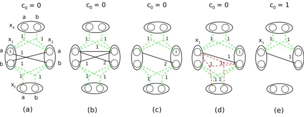
Example 2.4 Consider the four binary WCSPs in Figure2.5. Each WCSP has 2 variables i, j and a cost function cij. All variables have 2 values a, b. Contrary to CSPs, an arc in
a graph WCSP is used to indicate a tuple of positive cost. Numbers beside values and arcs represent respectively positive unary and binary costs while zero costs edges are not shown. These 4 problems are equivalent because they have the same valuation for every pair of values(a, b) ∈ D(i) × D(j) computed as cij(a, b) + ci(a) + cj(b) + c∅
a b a b 1 1 xi xj c∅= 0 (a) Ex(j, b, cij, 1) Pr(cij, j, b, 1) a b a b 1 xi xj c∅= 0 (b) Ex(i, b, cij, 1) Pr(cij, i, b, 1) a b a b 1 1 xi xj c∅= 0 (c) UPr(ci, 1) a b a b xi xj c∅= 1 (d)
Figure 2.5: Four equivalent WCSPs. An arrow from a WCSP A to a WCSP B means that B can be transformed from A by applying the EPT indicated above the arrow. Pr, Ex and UPr are respectively the cost projection, cost extension and unary cost projection on c∅.
Any operation that transforms a WCSP into an equivalent WCSP is called an Equiva-lence Preserving Transformation (EPT). The operation Shift(τS, cS′, α) presented in
Algo-rithm2.2 is such an EPT. It moves an amount of cost α between a cost function cS′ and
a tuple τS such that S is a subset of S′ and α can be negative or positive. Costs must
![Figure 2.4: Some examples for comparing AC, RPC, PIC, maxRPC [ Bessiere , 2006 ]. a)A CSP which is AC but is not RPC](https://thumb-eu.123doks.com/thumbv2/123doknet/2092516.7449/18.893.208.652.857.1037/figure-examples-comparing-rpc-pic-maxrpc-bessiere-csp.webp)