HAL Id: hal-01575285
https://hal.archives-ouvertes.fr/hal-01575285
Preprint submitted on 18 Aug 2017
HAL is a multi-disciplinary open access
archive for the deposit and dissemination of
sci-entific research documents, whether they are
pub-lished or not. The documents may come from
teaching and research institutions in France or
L’archive ouverte pluridisciplinaire HAL, est
destinée au dépôt et à la diffusion de documents
scientifiques de niveau recherche, publiés ou non,
émanant des établissements d’enseignement et de
recherche français ou étrangers, des laboratoires
A Core Theory of Delay Systems
Sébastien Boisgérault
To cite this version:
A Core Theory of Delay Systems
Sébastien Boisgérault
*July 9, 2017
Contents
Abstract 2 1 Introduction 32 The Initial Value Problem 4
2.1 Delay Operators . . . 4 2.2 Well-Posedness . . . 6 2.3 The FSA System . . . 9
3 Graph-Theoretic Analysis 10
3.1 Block Diagrams . . . 10 3.2 Causality Analysis . . . 12 3.3 Block Diagram of the FSA System . . . 15
4 Stability 15
4.1 Test in the Laplace Domain . . . 15 4.2 Stability of the FSA System . . . 18
Appendix 18
References 20
*MINES ParisTech, PSL Research University, Centre for Robotics, 60 Bd St Michel, 75006 Paris, France. E-mail: [email protected].
Abstract
We introduce a framework for the description of a large class of delay-differential algebraic systems, in which we study three core problems: first we characterize abstractly the well-posedness of the initial-value problem, then we design a practical test for well-posedness based on a graph-theoretic representation of the system; finally, we provide a general stability criterion. We apply each of these results to a structure that commonly arises in the control of delay systems.
1 Introduction
Systems of delay-differential algebraic equations (DDAE) combine differential and algebraic equations with delayed variables in the right-hand side. Among them, we represent linear and time-invariant systems with a finite memory r as
˙
x(t) = Axt+ Byt y(t) = Cxt+ Dyt
(1) where x(t) ∈ Rn, y(t) ∈ Rm and the notation z
t stands for the memory of
the variable z at time t: the function defined by zt(θ) = z(t + θ) for any θ ∈ [−r, 0]. The symbols A, B, C and D denote delay operators: linear and
bounded operators from the space of continuous functions C([−r, 0], Cj) toCi
for some integers i and j. Specifically, since (x(t), y(t))∈ Rn+m, we require that
the compound operator
[
A B C D
]
(2) is linear and continuous from C([−r, 0], Cn+m) toCn+m.
This description is general enough to encompass systems of seemingly different nature – such as ordinary differential equations (e.g. ˙x(t) = x(t)), delay systems of retarded type (e.g. ˙x(t) = x(t− 1)) or neutral type (e.g. ˙y(t) = ˙y(t − 1), rewritten as ˙x(t) = 0 and y(t) = x(t) + y(t− 1)), difference equations (e.g.
y(t) = y(t− 1)) but also different types of delays: systems with single delays
(e.g. ˙x(t) = x(t) + x(t− 1)), multiple delays (e.g. ˙x(t) = x(t − 1) + x(t − 2)),
distributed delays (e.g. ˙x(t) =∫tt−1x(θ) dθ) or a combination thereof. We refer
the reader to (Bensoussan et al. 2006, chap. 4) for a more comprehensive collection of examples.
However, competing theories of delay systems have been developped and used over time (Hale 1977; M. Delfour and Karrakchou 1987; Salamon 1984); they may use different definitions of delay operators, of the solutions to the initial-value problem and may be restricted to systems of a certain type. For the newcomer in the field, this is an unintended source of complexity. To make the subject more widely accessible, we lay out in this paper a simple but general framework for the description of delay systems, based on a combination of linear algebra and measure theory. Then we develop on this foundation a core theory: we characterize the well-posedness of the initial-value problem, then we perform a graph-theoretic analysis of this issue and finally, we provide a general stability criterion.
We illustrate the results of each section with the same example: the so-called finite spectrum assignment (FSA) architecture which is used for the control of dead-time systems (Manitius and Olbrot 1979). This example – and the methods
that we use to study it – are actually representative of a large class of controllers for delay systems which ranges from the primeval Smith predictor to the gen-eral observer-predictor structure (Mirkin and Raskin 2003). A linear dead-time systems is governed by an ordinary differential equation ˙x(t) = Ex(t) + F u(t) but the only information available at time t is the delayed variable x(t− T ). If
we apply the control u(t) = −Gy(t) where y(t) is the predicted value of x(t)
based on x(t− T ) and the history of u defined by y(t) = eT Ex(t− T ) +
∫ 0
−T
e−θEF ut(θ)dθ
then the closed-loop dynamics is ˙ x(t) = Ex(t)− F Gy(t) y(t) = eT Ex(t− T ) − ∫ 0 −T e−θEF Gyt(θ)dθ (3)
Since this system is not overly simplistic (it combines effectively differential and algebraic equations, its delays are discrete and distributed), it is a good testbed for the theory exposed in this paper.
2 The Initial Value Problem
2.1 Delay Operators
We have described general delays as operators applied to continous functions: if
C(X, Y ) denotes the space of continuous functions from X to Y , a delay operator
with memory length r is a bounded linear operator from C([−r, 0], Cj) to Ci
for some integers i and j. But delays also have two alternate (and equivalent) representations – as measures and as convolution kernels – which we will use extensively in the next sections.
We start with a quick example of these representations: consider y(t) = x(t− 1)
where x(t) is a scalar variable. We will associate to this delayed expression three distinct representations m1, m2 and m3 such that by construction
y(t) = m1xt= ∫ 0 −1 xt(θ) dm2(θ) = ∫ 1 0 x(t− θ)dm3(θ). (4)
The first one m1 is an operator applied to continuous scalar functions defined
on [−1, 0]; here, equation (4) clearly mandates that m1χ = χ(−1). The
measure at t =−1 and m3is δ1, the Dirac measure at t = 1. Now if instead we
consider the distributed delay y(t) =∫tt−1x(θ)dθ, equation (4) is satisfied with m1χ =
∫ 0
−1
χ(t) dt, m2= dt|[−1,0] and m3= dt|[0,1].
In general, we deal with vector-valued variables; in this broader context, the term “measure” may refer to several things. We use the term scalar measure for a complex-valued and countably additive function defined for the bounded Borel subsets of the real line (Fell and Doran 1988). A matrix-valued
mea-sure (resp. vector-valued meamea-sure) is a countably additive function defined for
the bounded Borel subsets of the real line whose values are complex matrices (resp. vectors) of a fixed size. Equivalently, it is as a matrix (resp. vector) whose
elements are scalar measures.
Given a matrix-valued measure L, we define the integral of the vector function
ϕ :R → Cj with respect to L as the vector ofCiwhose k-th element is given by ∀ k ∈ {1, . . . , j}, [∫ dL ϕ ] k = j ∑ l=1 ∫ ϕldLkl.
Riesz’s representation theorem provides a bijection between delay operators with memory length r and matrix-valued measures supported on [−r, 0]. We may
therefore use the same symbol L to denote both objects, and this convention yields for any ϕ∈ C([−r, 0], Cj)
Lϕ =
∫
dL ϕ.
The nature of the argument of L (function or set) determines without ambiguity which representation of L is used in a given context. When the argument is a set, we will also drop the parentheses when it improves readability: typically, instead of L({0}), we will use the lighter notation L{0}.
Let L∗ refer to the measure obtained by symmetry of the measure L around
t = 0, which is defined for any bounded Borel set B by L∗(B) = L(−B). This construct obviously provides a new bijection between delay operators with mem-ory length r and matrix-valued measures supported on [0, r], which is related to the representation of delay operators as convolutions.
We say that a measure µ is limited on the left if its support is included in [−r, +∞) for some r ∈ R, causal if its support is included in [0, +∞) and strictly
causal if additionally µ{0} = 0. The convolution µ ∗ ν of two scalar measures
limited on the left µ and ν is the scalar measure defined for any bounded Borel set B by
(µ∗ ν)(B) = ∫
The convolution of two vector or matrix-valued measures limited on the left combines the scalar convolution and the linear algebra product: for example, the convolution of two measures L and M with values inCi×j andCj×kis the
measure L∗ M, with values in Ci×k, given by
(L∗ M)(B)α,β=
j
∑
γ=1
(Lα,γ∗ Mγ,β)(B).
We may identify a (locally integrable) function f with the measure given by
f (B) =
∫
B f (t) dt.
This enables us to define the convolution of functions and measures, which may be identified with a function, and of two functions, which may be identified with an absolutely continous function. Additionally, we implicitly extend by 0 functions that are defined on a proper subset of real line – for example functions defined on [−r, 0] or [−r, +∞). With these conventions, if L is a delay operator
with memory r and ϕ∈ C([−r, +∞), Ci) then for almost every t > 0 Lϕt= (L∗∗ ϕ)(t).
2.2 Well-Posedness
Several concepts of solution exist for the problem formally described by
∀ t > 0 x(t)˙ = Axt+ Byt y(t) = Cxt+ Dyt
, (x(0), x0, y0) = (ϕ, χ, ψ). (5)
A classic (or continuous) solution is a pair of continuous functions (x, y) from [−r, +∞) to Cn+msuch that ˙x exists, is continous on (0, +∞) and satisfies the
system equations and initial conditions. In this setting, necessarily the functions
χ and ψ are continous, ϕ = χ(0) and the consistency condition ψ(0) = Cχ + Dψ
holds.
The continuity assumption ensures that the right-hand side of the system equa-tions is defined for any time t; if we relax this assumption, we may generalize the concept of solution to locally integrable solutions (Salamon 1984; M. Delfour and Karrakchou 1987).
Let L be a delay operator with memory length r and L∗ the corresponding convolution kernel. For any continuous function z defined on [−r, +∞), we
have Lzt = (L∗∗ z)(t) for any t > 0 but the right-hand side of this equation
locally integrable, a strong incentive to rewrite the initial value problem as a convolution equation. Using the Heaviside step function e, defined by
e(t) = 1 if t≥ 0,
0 otherwise,
we may also rewrite the (integral form of) the differential equation as a convo-lution equation. We end up with the following definition:
Definition – Solution of the Initial Value Problem. A pair of locally
integrable functions (x, y), defined on [−r, +∞), with values in Cn+m, is a (locally integrable) solution of the DDAE initial value problem (5) if
(x(0+), x0, y0) = (ϕ, χ, ψ)
and if there is a f ∈ Cn such that
[ x y ] (t) = [ e∗ A∗ e∗ B∗ C∗ D∗ ] ∗ [ x y ] (t) + [ f 0 ] for a.e. t > 0.
This definition makes sense even if the initial function data is not continuous, does not meet the consistency condition, or if χ(0)̸= ϕ. It is however consistent
with the concept of continuous solution when such solutions exist. The constant vector f is uniquely determined by the initial value: we have x(0+) = ϕ if and
only if f = ϕ− (e ∗ A∗∗ χ + e ∗ B∗∗ ψ)(0).
Now, because of its algebraic component, DDAE system (5) may have no solu-tions or multiple solusolu-tions; we may actually easily exhibit an algebro-differential system (with no delay) with this property. Consider
∀ t > 0, x(t)y(t)˙ == 0x(t) + y(t) (6) It is defined formally by n = 1, m = 1, for example r = 1 (any nonnegative value is admissible) and for any χ ∈ C0([−r, 0], Rn) and ψ ∈ C0([−r, 0], Rm), Aχ = 0, Bψ = 0, Cχ = χ(0), and Dψ = ψ(0). If x(0+) = 0, then x(t) = 0 for
t > 0 is the unique solution of the first system equation; the second equation
becomes y(t) = y(t), hence arbitrary values of y(t) for t > 0 satisfy it: multiple solutions exist. On the contrary, if x(0+) = 1, then necessarily x(t) = 1 for any
t > 0; the second equation would become y(t) = 1 + y(t), which no function y(t)
may satisfy: there are no solutions to this initial value problem.
A simple assumption that yields uniqueness of the solution is explicitness: a DDAE system is explicit if the right-hand side of its algebraic equation only depends strictly causally on the variable y, that is, if D{0} = 0. For example,
system (6) is not explicit since y(t) = x(t) + y(t) and thus D{0} = 1; replace
However this assumption is too conservative for some practical use cases, in-cluding the kind of sound composition of input-output systems that is exposed in the next section. Therefore we state in this section a well-posedness theorem applicable under a more general assumption that ensures that the system is merely equivalent to an explicit system.
Let Ip be the p× p identity matrix and X be the product space
X =Cn× L2([−r, 0], Cn+m). (7) endowed with the norm
∥(ϕ, χ, ψ)∥2 X=|ϕ| 2+ ∫ 0 −r|χ(t)| 2+|ψ(t)|2dt. (8)
Theorem – Well-posedness. DDAE systems such that Im−D{0} is invertible are well-posed in the product space X: when (ϕ, χ, ψ)∈ X, there is a unique so-lution (x, y) to the initial value problem (5), it belongs to L2
loc([−r, +∞), C
n+m), x is continuous and for any t > 0 there is some α > 0 such that
∥(x(t), xt, yt)∥X≤ α∥(ϕ, χ, ψ)∥X. (9) It is classic that this result holds when the system is explicit (Salamon 1984; M. Delfour and Karrakchou 1987; Boisgérault 2013). Therefore, to prove the general case, we only need to demonstrate the following lemma:
Lemma – Equivalent Systems. Assume that the matrix J := Im− D{0} associated to system (5) is invertible and denote E and F the delay operators E := J−1C and F := J−1(D− D|{0}). The original initial value problem and
the one defined by
∀ t > 0 x(t)˙ = Axt+ Byt y(t) = Ext+ F yt
, (x(0), x0, y0) = (ϕ, χ, ψ). (10)
have the same solutions but the latter system is always explicit:
F{0} = 0.
Proof. We may decompose the convolution kernel of D into two components:
D∗= (D|[−r,0])∗= (D|{0})∗+ (D|[−r,0))∗.
The first component is instantaneous: for any locally integrable function y ((D|{0})∗∗ y)(t) = D{0}y(t);
the second component is strictly causal:
(D|[−r,0))∗{0} = D|[−r,0){0} = 0.
Consequently, a pair of locally integrable functions (x, y) : [−r, +∞) → Rn+mis
a solution of the DDAE system equations (5) if and only if they satisfy, almost everywhere for t > 0, the equations
x(t) = (A∗∗ x)(t) + (B∗∗ y)(t) + f
y(t)− D{0}y(t) = (C∗∗ x)(t) + ((D|[−r,0))∗∗ y)(t)
By assumption the matrix J = Im−D{0} is invertible, thus the second equation
is equivalent to
y(t) = (E∗∗ x)(t) + (F∗∗ y)(t)
with E = J−1C and F = J−1D|[−r,0). The functions x and y are solutions
of the original DDAE system if and only if they are solutions – with the same initial values – of the system whose delay operators are A, B, E and F . This new DDAE system is explicit by construction: F{0} = J−1D|
[−r,0){0} = 0. ■
2.3 The FSA System
The delay operators A, B and C of system (3) are defined by Axt = Ex(t), Byt = −F Gy(t) and Cxt = eT Ex(t− T ). Since the Dirac measure δτ at τ ∈ R satisfies δτφ = φ(τ ), we have A = Eδ0, B = −F Gδ0, C = eT Eδ−T
or equivalently
A∗= Eδ0, B∗=−F Gδ0, C∗= eT EδT. (11)
The fourth delay operator D is defined by
Dyt=−
∫ T
0
eθEF Gy(t− θ)dθ = −(eθEF Gdθ|[0,T ]∗ y)(t),
hence D∗=−eθEF Gdθ|[0,T ]. (12) In particular D∗{0} = − ∫ {0} eθEF Gdθ = 0,
3 Graph-Theoretic Analysis
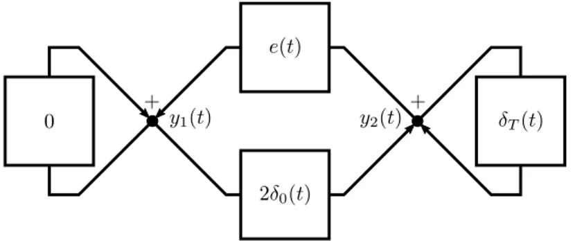
Block diagrams used in control theory provide an alternative to the system-of-equations approach for the modelling of dynamical systems: in this context, dynamical systems are specified as diagrams made of blocks and wires as in figure 1. Blocks are independent input-output systems with their own behaviors: each block specifies how to compute the values of its output variables given the values of its input variables (and optionally of some local initial state). In figure 1, each rectangle is a block and the symbol it holds defines its behavior. Wires connect these blocks to build larger systems: they specify how the input of each block is computed as a combination of the outputs of all blocks.
Figure 1: Block diagram of a simple delay system.
This classic description – actually a graph representation in disguise – offers new indsights into the structural properties of dynamical systems. In section 3.1, we complete for delay systems the informal definition of block diagrams that we have given so far and expose the connexion with graph theory. Then, in section 3.2, we focus on causality to design sound composition rules of subsystems, that ensure the well-posedness of the initial-value problem for the global system.
3.1 Block Diagrams
For linear time-invariant systems, block diagrams can always be decomposed into elementary input-output systems with a scalar input u(t) and a scalar out-put y(t), defined for t > 0, and characterized by a scalar convolution kernel
k∗. Additionally, for delay systems, only two types of elementary subsystems are required: the integrator, whose kernel is the Heaviside step function e, and (scalar) finite-memory delay operators. By definition, the behavior of an
ele-mentary system is governed by
y(t) = (k∗∗ u)(t) + (k∗∗ ω)(t), t > 0;
where ω, a scalar function defined on [−r, 0] that represents a finite memory of
A block diagram embeds a collection of such systems into a (directed, labeled) graph structure: each vertice i refers to an output variable yiand each edge j→ i is labeled with a scalar kernel k∗= Kij∗; the global initial state is determined by the collection of functions ωij for every edge j→ i. The functional analytic
representation of this system is
yi(t) = ∑ j (Kij∗ ∗ yj)(t) +∑ j (Kij∗ ∗ ωij)(t), t > 0. (13) For example, the block diagram depicted in figure 1 has two nodes – associated to variables y1 and y2 – and four edges – whose labels are K11∗ = 0, K12∗ = e,
K21∗ = 2δ0 and K22∗ = δT. Then y1(t), defined for t > 0, satisfies
y1(t) = (0∗ y1)(t) + (e∗ y2)(t) + (0∗ ω11)(t) + (e∗ ω12)(t)
= (e∗ y2)(t) + (e∗ ω12)(t)
which, since (e∗ ω12)(t) is a constant c for t > 0, is the integral form of the
differential equation ˙y1(t) = y2(t) with initial value y1(0) = c. On the other
hand y2(t), also defined for t > 0, satisfies
y2(t) = (2δ0∗ y1)(t) + (δT ∗ y2)(t) + (2δ0∗ ω21)(t) + (δT ∗ ω22)(t)
and since (2δ0∗ω21)(t) = (δT∗ω22)(t) = 0 for any t > r, eventually the equation
y2(t) = 2y1(t) + y2(t− T ) holds and the behavior of the system is ruled by a
DDAE system. This is not accidental, since the following result holds:
Theorem. Every DDAE system has a canonical block diagram representation. Proof. Suppose that for some constant vector f
x(t) = (e∗ A∗∗ x)(t) + (e ∗ B∗∗ y)(t) + f
y(t) = (C∗∗ x)(t) + (D∗∗ y)(t) , t > 0
and
(x(0+), x|[−r,0], y|[−r,0]) = (ϕ, χ, ψ).
The vector f is uniquely determined by the initial state. We may define the auxiliary variable w(t) for t > 0 by w(t) = (A∗∗ x)(t) + (B∗∗ y)(t), and rewrite
the first equation of the DDAE system as
x(t) = (e∗ w)(t) + (e ∗ υ)(t), t > 0
for any function υ : [−r, 0] 7→ Cn such that (e∗ υ)(0) = f. It is now plain that
the variable z(t) = (x(t), w(t), y(t)) defined for t > 0, the matrix kernel and the initial state K∗= A0∗ eIn0 B0∗ C∗ 0 D∗ , ωij = (χ, υ, ψ)j (14)
satisfy zi(t) =∑ j (Kij∗ ∗ zj)(t) + ∑ j (Kij∗ ∗ ωij), t > 0. (15)
which is the functional analytic representation of a block diagram. ■
3.2 Causality Analysis
We say that a scalar input-output system is causal (resp. strictly causal) if its convolution kernel is causal (resp. strictly causal). For example, since the kernel of the integrator is the function e, it is strictly causal:
e{0} =
∫
{0}
e(t) dt = 0.
A (discrete or pure) delay of T > 0 seconds satisfies y(t) = u(t− T ); its kernel
is k∗= δT and it is strictly causal. Similarly, a distributed delay with bounded
delay r, defined by the equation
y(t) =
∫ 0
−r
h(θ)u(t + θ)dθ
for some locally integrable function h : [−r, 0] → R, is also strictly causal. A
gain y(t) = ku(t) is causal, but it is strictly causal only if k = 0.
Definition – Causality Loop. A causality loop of a block diagram with kernel
matrix K∗of size n× n is a finite sequence of integers i0, i1, . . . , ij in{1, . . . , n}
such that i0 = ij and for any ℓ ∈ {0, . . . , j − 1}, the system with kernel k∗ℓ = Ki∗
ℓ+1iℓ is not strictly causal.
The block diagram of figure 1 has no causality loop, since the only element of its matrix K∗ which is not strictly causal is K21∗ = 2δ0 which is not on the matrix
diagonal. The following result is applicable in this case:
Theorem. If the block diagram representation (14)-(15) of DDAE system (5)
has no causality loop then D{0} is nilpotent.
Proof. Let K∗ be the kernel matrix of the block diagram representation of DDAE system (5). In this proof, for any matrix-valued measure M , we denote
M0 the matrix M{0}. Let A[K] be the adjacency matrix of the block diagram
directed graph, stripped off its strictly causal edges:
A[K]ij = 1 if [K0]ij̸= 0 0 otherwise.
The graph-theoretic concept of loop corresponds to our definition of causality loop. Element (i, j) of the p-th power A[K]p of the adjacency matrix is the
number of distinct paths with p edges between vertices j and i. If there is a loop of length p in the block diagram, there is also a loop whose length is an arbitrary multiple of p, hence the adjacency matrix is not nilpotent. Conversely, if the adjacency matrix is not nilpotent, there is a pair (i, j) such that A[K]n
ij ̸= 0;
since any path between j and i goes through n + 1 vertices and the graph has only n distinct vertices, at least one of them is repeated: the path necessarily contains a loop.
Now, ifA[K]p= 0 for some p∈ N∗ then [K
0]p= 0. Indeed, since A[K]p ij = ∑ ℓ1,...,ℓp−1 A[K]iℓ1. . .A[K]ℓp−1j
and all elements of the adjacency matrix are non-negative, if its p-th power is zero, there is for each term in the sum above at least one factorA[K]νµwhich is zero and thus [K0]pνµ= 0. Consequently, since
[K0] p ij = ∑ ℓ1,...,ℓp−1 [K0]iℓ1. . . [K0]ℓp−1j,
the p-th power of K0 is also zero. But for any integer p≥ 2, we have
[K0]p= A00 00 B00 C0 0 D0 p = B0[D00]p−2C0 00 B0[D00]p−1 [D0]p−1C0 0 [D0]p . Consequently, if the block diagram has no causality loop,A[K] is nilpotent and
the matrix D0= D{0} is also nilpotent. ■
Note that the absence of causality loop does not necessarily provide explicitness: for example, the delay operator D of the DDAE system governed by y1(t) = y2(t)
and y2(t) = y1(t− 1) satisfies D{0} = [ 0 1 0 0 ]
which is not zero. However, it is plain that its block-diagram representation has no causality loop: it contains only one subsystem which is not strictly causal and this subsystem connects variable y1 to the other variable y2. This is sufficient
to ensure its well-posedness:
Corollary. A DDAE system without causality loop is well-posed.
Proof. If DDAE system (5) has no causality loop, the matrix D{0} is nilpotent
and [D{0}]m= 0. Consequently, the matrix I
m− D{0} is invertible:
[Im− D{0}]−1 = Im+ D{0} + · · · + [D{0}]m−1.
Integrator
Pure Delay
Distributed Delay
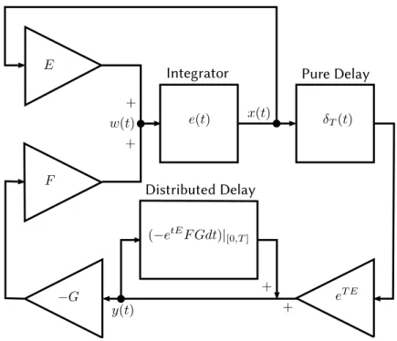
Figure 2: FSA closed-loop system block diagram. Each rectangular block char-acterizes an input-output system by its (function or measure) convolution kernel. A triangle with symbol K represents a gain: a system whose output y(t) and input u(t) satisfy y(t) = Ku(t).
3.3 Block Diagram of the FSA System
In the block diagram representation of system (3), the auxiliary variable w satisfies
w(t) = Ex(t)− F Gy(t), t > 0.
Since x(t) = e∗ w(t) + e ∗ υ(t) is the only (system of) equation(s) with some
variable wj in the right-hand side or some variable xi in the left hand-side,
there is a unique outgoing edge of wj (with a nonzero label) which is also the
unique incoming edge of the variable xj. This label is the function e, strictly
causal, thus no causality loop may contain either of the components of the state variables w or x. Now the possible causality loops that could remain would contain only vertices which are components of the state variable y. But the edge between yjand yi is Hij∗ where H∗= (−e
tEF Gdt)|
[0,T ]. Again, this kernel
is a function and hence is strictly causal. Thus no such loop may exist and the initial-value problem is well-posed.
This analysis may also be carried out graphically on figure 2. Once the in-tegrator, the pure delay and the distributed delay – which are strictly causal subsystems – are removed from the diagram, it is plain that there is no loop and thus that the system has no causality loop.
4 Stability
4.1 Test in the Laplace Domain
There is a general and simple test in the Laplace domain for the exponential stability of a DDAE system. It can also be used to determine its growth bound, defined as the infimum of the σ+ such that for any initial value, there is a
κ > 0 such that the solution satisfies ∥(x(t), xt, yt)∥X ≤ κeσ+t for any t > 0; exponential stability corresponds to a negative growth bound.
A few definitions are in order first: the Laplace transformLL of a compactly
supported measure L is the function defined onC by
LL(s) =
∫
e−stdL(t).
The Laplace transform of L∗ satisfiesLL∗(s) = L(t 7→ est). The characteristic matrix of the system is then defined as
∆(s) = [ sIn 0 0 Im ] − L [ A∗ B∗ C∗ D∗ ] (s) (16)
We may now state the criterion:
Theorem. The growth bound σ of a DDAE system without causality loop is:
σ = sup{ℜ(s) | s ∈ C, det ∆(s) = 0}. (17) The proof of this theorem is carried out in (Boisgérault 2013) in the case of explicit systems. Here, we expose the proof in the general case.
Lemma. DDAE systems (5) and (10) have simultaneously singular
character-istic matrices ∆(s) and ∆†(s).
Proof. Let J = Im− D{0}, E = J−1C and F = J−1(D− D|{0}); we have LE∗= J−1LC∗ and LF∗= J−1(LD∗− D{0})
and since Im+ J−1D{0} = J−1, Im− LF∗= J−1(Im− LD∗). Finally,
∆†(s) = [ sIn 0 0 Im ] − L [ A∗ B∗ E∗ F∗ ] (s) = [ In 0 0 J−1 ] ∆(s) and the characteristic matrices are simultaneously singular. ■ The determinant and adjugate of the characteristic matrix ∆† have a quasi-polynomial structure: det ∆†(s) = n ∑ i=0 ci(s)si, adj ∆†(s) = n ∑ i=0 Ci(s)si (18)
where the ci (resp. Ci) are entire functions (resp. matrices of entire functions)
bounded on any right-hand plane. It is plain that the leading coefficient of the characteristic function is given by cn(s) = det ∆0(s) where ∆0 is the
character-istic matrix of the system y(t) = F yt.
Lemma – Zero Clusters. Let Hσbe the open right half-plane{s ∈ C | ℜ(s) > σ} and let Zη be the set of points whose distance to the zeros of det ∆0 is at
most η.
For any σ∈ R and ϵ > 0, there is a η > 0 such that:
i. any connected component Λ of the set Zη is bounded,
ii. Λ is a subset of Hσ−ϵ whenever Λ∩ Hσ ̸= ∅,
iii. | det ∆0| has a positive lower bound on Hσ−ϵ\ Zη.
The proof (from (Boisgérault 2013)) is given in the appendix for the sake of completeness.
Lemma – Characteristic Function Zeros. Let σ∈ R. If the function det ∆0
has an infinite number of zeros on Hσ, the function det ∆†has an infinite number of zeros on Hσ−ϵ for any ϵ > 0.
Proof. Suppose that det ∆0 has an infinite number of zeros in Hσ and let η > 0 be as in the zero clusters lemma. The zeros of det ∆0 are isolated, thus
the collection of components Λ of Zη such that Λ∩ Hσ ̸= ∅, which is locally
finite by construction, is also infinite: for any compact set K, there is a Λ such that Λ∩ K = ∅.
Since det ∆†(s) has a quasi-polynomial structure with leading coefficient det ∆0(s) sn and since det ∆0(s) has a positive lower bound on Hσ−ϵ \ Zη,
there is a compact set K such that | det ∆†(s)− sndet ∆
0(s)| < |sndet ∆0(s)|
whenever s∈ Hσ−ϵ\ Zη and s̸∈ K. Rouché’s theorem is applicable to any of the components Λ in the complement of K, each of which contains at least one zero of det ∆0. Thus, det ∆† has an infinite number of zeros in Hσ−ϵ. ■
We can associate to the initial-value problem (5), or (10) which is equivalent, a one-parameter family of operators (exp(At))t≥0 defined by
(x(t+), xt, yt) = exp(At)(ϕ, χ, ψ) for t ≥ 0, (ϕ, χ, ψ) ∈ X.
It is a strongly continous semigroup on the product space X; its infinitesimal generatorA is defined by
A(ϕ, χ, ψ) = (Aχ + Bψ, ˙χ, ˙ψ)
on the domain
{(ϕ, χ, ψ) ∈ Cn× W1,2([−r, 0], Cn+m)| χ(0) = ϕ, ψ(0) = Eχ + F ψ}.
The resolvent operator (sI−A)−1exists if and only if ∆†(s) is non-singular and
moreover, for any real number σ there are constants κσ and λσ such that
∥(sI − A)−1∥ ≤ κσ∥∆†(s)−1∥ + λσ (19)
ifℜs ≥ σ and det ∆†(s)̸= 0 (see Salamon (1984)).
We may now prove the main result:
Proof. Let s(A) be the spectral bound of A. We show that for any σ > s(A), ∥∆†(s)−1∥ is bounded on Hσ. Thus, by inequality (19),∥(sI−A)−1∥ is similarly
bounded and the Gearhart-Prüss theorem proves the result.
The quasi-polynomial structure of the adjugate matrix provides for some κ≥ 0
∥adj ∆†(s)∥ ≤ κ(1 + |s|n)
on Hσ. Since the resolvent operator is defined on Hσ−ϵ for any ϵ > 0 such that s(A) < σ − ϵ, det ∆† has no zero in Hσ−ϵ. Thus, by the characteristic function
zeros lemma, det ∆0 has at most a finite number of zeros on Hσ−ϵ/2 and thus
has a positive lower bound κ′. It follows from the quasipolynomial structure of det ∆† that
| det ∆†(s)| ≥ κ′
2(1 +|s|
n)
on Hσ except on some compact set K; by continuity of det ∆†, this estimate
still holds on all of Hσ with a possibly smaller κ′. Finally, for any s ∈ Hσ, ∥∆†(s)−1∥ = ∥adj ∆†(s)∥/| det ∆†(s)| ≤ 2κ/κ′. ■
4.2 Stability of the FSA System
Since the kernels of FSA system (3) are given by (11) and (12), its characteristic matrix satisfies
∆(s) = [
sIn− E F G −e(sIn−E)T In+ P (s)F G
]
where P (s) is the analytic extension to C of the meromorphic function
s7→ [sIn− E]−1(In− e(sIn−E)T).
A straightforward computation provides ∆(s) [ In 0 In In ] = [ sIn− E + F G F G P (s)(sIn− E + F G) In+ P (s)F G ]
and the right-hand side of this equation can be factored into [ In 0 P (s) In ] [ In F G 0 In ] [ sIn− E + F G 0 0 In ] .
Thus, the characteristic function satisfies
det ∆(s) = det(sIn− E + F G)
and it roots are the eigenvalues of E− F G. When the delay-free system ˙x(t) = Ex(t) + F u(t) is controllable, finite-dimensional control theory provides a gain
matrix G that assigns these eigenvalues to n arbitrary locations in the complex plane, and thus we may achieve a “finite spectrum assignment” of the closed-loop system. In particular, it’s possible to select a gain matrix G which exponentially stabilizes system (3).
Appendix
We provide in this appendix a proof of the zero clusters lemma. First we derive some properties of det ∆0by expressing it as the Laplace transform of a complex
measure µ. Let Σm be the set of permutations of{1, ..., m} and
det∗M = ∑ σ∈Σm
sgn(σ)M1,σ(1)∗ . . . ∗ Mm,σ(m).
As ∆0(s) = Im−LF∗(s), det ∆0=Lµ where µ = det∗(δ0Im−F∗). The complex
measure µ is a sum of convolution products of m complex measures supported on [0, r], hence it is supported on [0, mr]. Consequently, det ∆0 is an entire
function that satisfies the inequality
| det ∆0(s)| ≤ |µ|([0, mr]) max(1, exp(−ℜ(s)mr)). (20)
Since F{0} = 0, we also have µ{0} = 1, which yields
lim
ℜs→+∞det ∆0(s) = 1. (21)
We may now proceed to the proof:
Proof (Zero Clusters Lemma). The function z 7→ det ∆0(iz) meets the
assumptions of theorem VIII in (Levinson 1940) and is of exponential type mr. Thus, the number of distinct zeros N (ρ) of det ∆0whose modulus is less than ρ is
such that lim supρ→+∞N (ρ)/ρ≤ 2mr/π. If the component of Zη that contains
a zero s is unbounded, there are at least n + 1 zeros in the closed disk centered at s of radius 2ηn and thus lim supρ→+∞N (ρ)/ρ ≥ 1/2η. Consequently, if η < π/4mr, every connected component of Zη is bounded.
The proofs of statements ii. and iii. use a similar argument. In each case we consider a sequence sn of complex numbers of bounded real part and the
func-tions fn(s) = det ∆0(s + iℑsn). Since inequality (20) holds, these functions are
locally uniformly bounded, hence there is a subsequence of sn which converges
to some real number x and, by Montel’s theorem, a corresponding subsequence of fn that converges locally uniformly to an entire function f∞. By (21), f∞is
not identically zero, thus by Hurwitz’s theorem, if m is the multiplicity of x if
f∞(x) = 0, or 0 otherwise, for any sufficiently small δ > 0, det ∆0 has exactly
m zeros in the open disk B(sn, δ) for an infinite number of values of n.
To prove ii., we assume the existence of a sequence Λn of connected components
of Zηn where ηn → 0 and such that Λn∩ Hσ ̸= ∅ but Λn ̸⊂ Hσ−ε. The Λn
are eventually bounded and there is a tuple of zeros in Λn with a first element
such thatℜs + ηn > σ, a last element such thatℜs − ηn≤ σ − ϵ and a distance
between consecutive points that is at most 2ηn. Let sn to be the first element
of this tuple; the real part of this sequence is bounded by (21). But for any
δ > 0, the number of zeros in B(sn, δ) converges to +∞, a contradiction with
the previous paragraph.
To prove iii., we assume the existence of a sequence sn in Hσ−ϵ\ Zη such that
we may select sn such that ℜsn → x. Now, f∞(x) = limn→+∞fn(ℜsn) = 0,
thus for some δ < η and for some value of n, there is at least one zero of det ∆0
in B(sn, δ), which is a contradiction. ■
References
Bensoussan, Alain, Giuseppe Da Prato, Michel C. Delfour, and Sanjoy K. Mitter. 2006. Representation and Control of Infinite Dimensional Systems (Systems &
Control: Foundations & Applications). Birkhauser.
Boisgérault, Sébastien. 2013. “Growth bound of delay-differential algebraic equations.” C. R., Math., Acad. Sci. Paris 351 (15-16). Elsevier
(Else-vier Masson), Issy-les-Moulineaux; Académie des Sciences, Paris: 645–48. doi:10.1016/j.crma.2013.08.001.
Delfour, M.C., and J. Karrakchou. 1987. “State space theory of linear time invariant systems with delays in state, control, and observation variables. I, II.”
Journal of Mathematical Analysis and Applications.
Fell, J.M.G., and R.S. Doran. 1988. Representations of *-algebras, locally
compact groups, and Banach *- algebraic bundles. Vol. 1: Basic representation theory of groups and algebras. Boston, MA etc.: Academic Press, Inc.
Hale, J. K. 1977. Theory of Functional–differential Equations. Springer–Verlag, Berlin–Heidelberg–New York.
Levinson, Norman. 1940. Gap and density theorems. American Mathematical Society (AMS). Colloquium Publications. 26. New York: American Mathemat-ical Society (AMS). VIII, 246 p.
Manitius, Andrzej Z., and Andrzej W. Olbrot. 1979. “Finite spectrum assign-ment problem for systems with delays.” IEEE Trans. Autom. Control 24: 541–53. doi:10.1109/TAC.1979.1102124.
Mirkin, Leonid, and Natalya Raskin. 2003. “Every stabilizing dead-time con-troller has an observer-predictor-based structure.” Automatica 39 (10): 1747–54. doi:10.1016/S0005-1098(03)00182-1.
Salamon, D. 1984. Control and observation of neutral systems. Research Notes in Mathematics, 91, Boston-London-Melbourne: Pitman Advanced Publishing Program. 207 p.