Revisiting Value Prediction

(1)

HAL Id: hal-00758713

https://hal.inria.fr/hal-00758713

Submitted on 29 Nov 2012

HAL is a multi-disciplinary open access

archive for the deposit and dissemination of

sci-entific research documents, whether they are

pub-lished or not. The documents may come from

L’archive ouverte pluridisciplinaire HAL, est

destinée au dépôt et à la diffusion de documents

scientifiques de niveau recherche, publiés ou non,

émanant des établissements d’enseignement et de

Arthur Perais, André Seznec

To cite this version:

Arthur Perais, André Seznec. Revisiting Value Prediction. [Research Report] RR-8155, INRIA. 2012,

pp.22. �hal-00758713�

(2)

0249-6399 ISRN INRIA/RR--8155--FR+ENG

RESEARCH

REPORT

N° 8155

November 2012

Prediction

Arthur Perais, André Seznec

(3)

(4)

RESEARCH CENTRE

RENNES – BRETAGNE ATLANTIQUE

Arthur Perais, André Seznec

Project-Team ALF

Research Report n° 8155 — November 2012 — 22 pages

Abstract: Value prediction was proposed in the mid 90’s to enhance the performance of high-end microprocessors. Unfortunately, to the best of our knowledge, there are no Value Prediction implementations available on the market. Moreover, the research on Value Prediction techniques almost vanished in the early 2000’s as it was more effective to increase the number of cores than to dedicate silicon to Value Prediction. However, high-end processor chips currently feature 8-16 high-end cores and the technology will allow to implement 50-100 of such cores on a single die in a foreseeable future. Amdahl’s law suggests that the performance of most workloads will not scale to that level. Therefore, dedicating more silicon area to single high-end core will be considered as worthwhile for future multicores, either in the context of heterogeneous multicores or homogeneous multicore. In particular, spending transistors on specialized, performance and/or power optimized units, such as a value predictor. In this report, we first build on the concept of value prediction. We introduce a new value predictor VTAGE harnessing the global branch history. VTAGE directly inherits the structure of the indirect jump predictor ITTAGE. We show that VTAGE is able to predict with a very high accuracy many values that were not correctly predicted by previously proposed predictors, such as the FCM predictor and the stride predictor. Compared with these previously proposed solutions, VTAGE can accommodate very long prediction latencies. The introduction of VTAGE opens the path to the design of new hybrid predictors. Three sources of information can be harnessed by these predictors: the global branch history, the differences of successive values and the local history of values. We show that the predictor components using these sources of information are all amenable to very high accuracy at the cost of some prediction coverage. Using SPEC 2006 benchmarks, our study shows that with a large hybrid predictor, in average 56.76% of the values can be predicted with a 99.48% accuracy against respectively 55.50%and 98.62% without advanced confidence estimation and the VTAGE component. Key-words: Value Prediction, VTAGE, hybrid predictors

(5)

formance des processeurs haut de gamme. Malheureusement, à notre connaissance, aucune implémentation n’est disponible sur le marché. De plus, la recherche dédiée aux techniques de prédiction a presque disparue au début des années 2000 car il était plus intéréssant d’augmenter le nombre de cœurs que de dédier du silicium à cette technique. Cependant, les processeurs haut de gamme possèdent de nos jours 8 à 16 cœurs et les progrès technologiques futurs permettront d’implémenter 50 à 100 cœurs similaires aux cœurs actuels sur une seule puce. De plus, la loi d’Amdahl suggère que la performance de la majorité des programmes ne passera pas à l’échelle sur un tel nombre de cœurs. Conséquemment, dédier plus de surface de silicium à un unique cœur haute performance sera considéré comme digne d’intérêt pour les futurs multicœurs, que ce soit dans le contexte des multicœurs hétérogènes ou homogènes. En particulier, dépenser des transistors dans des unités optimisées pour la performance et/ou la consommation, tel qu’un prédicteur de valeur. Dans ce rapport, nous commençons par augmenter le concept de prédic-tion de valeurs. Nous introduisons un nouveau prédicteur de valeur VTAGE tirant parti de l’historique global de branchement. VTAGE hérite directement de la structure du prédicteur de sauts indirects ITTAGE. Nous montrons que VTAGE est capable de prédire avec une très haute précision un grand nombre de valeurs n’étant pas prédites correctement par les prédicteurs proposés précédemment, tels que le prédicteur FCM ou le prédicteur Stride. Contrairement à ces solutions, VTAGE n’est pas impacté par la latence de la prédiction. L’introduction de VTAGE rend aussi possible l’utilisation de nouveaux prédicteurs hybrides. Trois sources d’informations peuvent être utilisées par ces prédicteurs : L’historique global de branchement, la différence en-tre les valeurs successivement produites et l’historique local des valeurs. Nous montrons que les composants utilisant ces sources d’informations peuvent tous atteindre une très haute précision au prix d’une perte de couverture. En utilisant des benchmarks de la suite SPEC 2006, notre étude montre qu’avec un grand prédicteur hybride, en moyenne 56.76% des valeurs peuvent être prédites avec une précision de 99.48%, contre respectivement 55.50% et 98.62% sans notre méchanisme d’estimation de confiance avancé et VTAGE.

(6)

1 Introduction

Around 2020, IC technology might allow to build processor chips integrating 50-100 superscalar cores. Intrinsically parallel workloads strongly benefit from additional cores. Yet the software industry is moving towards parallel applications at a relatively slow pace, while Amdahl’s law [1] emphasizes the need for performance on sequential code sections. Dedicating more silicon area to single thread performance is becoming worth to reconsider either in the context of heterogeneous multicores, as suggested in [7] or in the context of homogeneous general-purpose multicores. Some architectural techniques were proposed in the late 90’s for high-end uniprocessor but were not implemented at the beginning of the multicore era; among these techniques was Value Prediction [10], which we revisit in this paper.

Superscalar processors leverage Instruction Level Parallelism (ILP) to increase sequential performance by concurrently executing several independent instructions from the same control flow. However, ILP is limited and no more than a few instructions can be executed in parallel [6]. This is due to both control and data dependencies between instructions in the code. As a consequence, being able to break these dependencies might be leveraged for direct sequential performance gains.

To accommodate control dependencies, Branch Prediction is universally used in processor design. The processor can continue fetching instructions speculatively ignoring control depen-dencies. Similarly, on out-of-order execution processors, Register Renaming is used to truly remove false data dependencies (Write-After-Write and Write-After-Read) on registers. How-ever, nowadays true data dependencies (Read-After-Write) on registers are always enforced by stalling the pipeline.

Lipasti et al. proposed Value Prediction [10] to speculatively ignore true register RAW dependencies. By speculating on the result of instructions, Value Prediction allows for early speculative execution of instructions requiring the predicted value. Value Prediction leverages Value Locality, that is the observation that dynamic instructions tend to produce results that were already generated by a previous instance of the same static instruction [10]. Value Prediction is usually approached as a way to further improve sequential performance by implementing it in a state of the art pipeline. However, it should be noted that instead of aiming for the ultimate sequential performance, Value Prediction can also be viewed as an alternative to out-of-order execution [13].

Previous work in this field led to moderately to highly accurate predictors [11, 15, 18]. How-ever, accuracy was shown to be critical due to misprediction penalties [19]. If no selective replay is implemented then the penalty of a value misprediction can be as high as the cost of a branch misprediction. Therefore, even a slight drop in accuracy might lead to a big performance loss.

In this paper, we present a new value predictor component: The Value TAGE predictor (VTAGE). This predictor leverages the global branch history and is amenable to very high confidence. We show that VTAGE captures some value predictability that is captured neither by previously proposed value predictors leveraging local value history nor by stride-based predictors. Consequently, we show that one can build very accurate predictors with high prediction coverage through combining a local value history predictor, a stride value predictor and VTAGE.

The remainder of this paper is organized as follow: Section 2 describes related work. Section 3 introduces our new value predictor component, VTAGE. In Section 4, we describe how to improve all the predictors in order to achieve very high accuracy on high confidence predictions. Section 5 summarizes our evaluation methodology while Section 6 details the results we obtained. Finally, Section 7 provides some directions for future research.

(7)

2 Related Work

2.1 Value Predictors

Lipasti and Shen introduced Value Locality in [9, 10]. Value Locality states that a given dynamic instruction is likely to produce a result that was also produced by a previous instance. Value Locality exists for both instruction results and effective addresses. They propose the last value prediction (LVP), which consists in always predicting that the result of an instruction is the result produced by the last instance of the corresponding static instruction.

Sazeides and Smith defined two types of value predictors in [15]. On the one hand, Com-putational predictors generate a prediction by applying a function to the value(s) produced by the previous instance(s) of the instruction. For instance, the Last Value predictor uses the iden-tity function while a Stride predictor uses the addition of a constant (stride) as its function. A Two-Delta Stride [4] predictor is similar except for the fact that it uses two strides: one stride is always updated and the second stride is only updated if the first stride has seen the same value two consecutive times. The latter is used to make the prediction.

On the other hand, Context-Based predictors rely on patterns in the value history of a given static instruction to generate the speculative result of the current instance. The main representatives of this category are Finite Context Method predictors (FCM). Such predictors are usually implemented as two levels structures. The first level (Value History Table or VHT) records a value history - possibly compressed - and is accessed using the instruction address. The history is then hashed to form the index of the second level (Value Prediction Table or VPT), which contains the actual prediction. A confidence estimation mechanism is usually added in the form of saturating counters in either the first level table or the second level table [2, 14]. These two families of value predictors are complementary to some extent since they are expert at predicting distinct instructions.

Real implementations of FCM-like predictors may be very difficult because several instances of the same instructions might be in the pipeline at the same time. Consequently, a speculative history must be kept for each in-flight instruction.

Nakra et al. use global branch history for predicting values [11]. The Per-Path Stride pre-dictor (PS) is a stride-based prepre-dictor using the global branch history to select the stride to be added to the result produced by the last instance. First, the instruction address is used to access the last value in the Value History Table (VHT), while the stride is selected in the Stride History Table (SHT) using a hash of the history and the PC. Then, the two values are added to form the prediction.

Yet, to accommodate the misprediction recovery, value predictors must be very accurate. In [19], Zhou et al. showed that even when using a very smart mechanism to handle recovery (namely selective replay), accuracy is still fundamental to benefit from Value Prediction. Even in the idealistic case where faulting instructions can get back in the reissue queue in only one cycle, the average speedup nearly vanishes as the misprediction rate increases from 0% to 15%. Granted a conventional confidence mechanism, we found that existing predictors can manage to reach around 96% accuracy. However, bridging the gap between 96 and 99% is necessary to reach speedups in accordance with the cost of Value Prediction. This observation gets even more relevant as the width and the depth of the pipeline grows, since more and more instructions can be in flight at a given instant.

2.2 Indirect Jump Target Prediction

The prediction of the results of particular instructions, namely indirect jumps, has received a particular attention. Since our VTAGE predictor is directly derived from the ITTAGE predictor

(8)

[17], we detail the latter.

It has been observed that most of the correlations between branches are found between close ones (in terms of dynamic branch instructions executed), and fewer correlations are found be-tween distant branches. However, to achieve high accuracy and coverage, capturing correlations between distant branches is necessary. Seznec proposed the TAgged GEometric predictor in [17] to fulfill this very requirement. This scheme is well suited for branch prediction but also for indirect branch target prediction, as demonstrated by the ITTAGE predictor [17].

The idea is to have several tables - components - storing predictions. Each table is indexed by a different number of bits of the global branch history, hashed with the PC of the branch instruction. The different lengths form a geometric series. These tables are backed up by a base predictor, which is accessed using only the instruction address. In ITTAGE, an entry of a tagged component consists of a partial tag, a 1-bit usefulness counter u used by the replacement policy, a full address targ giving the prediction and a 2-bit hysteresis counter ctr. An entry of the base predictor simply consists of the prediction and the hysteresis counter.

When a prediction must be provided, all components are accessed in parallel to check for a hit. The component with a hit accessed with the longest history is called the provider component. It will provide the prediction to the pipeline. The component that would have provided the prediction had there been a miss in the provider component is called the alternate component. In some cases, it is more interesting to take the prediction of the alternate component (e.g. when the provider entry was allocated recently). This property is monitored by a global counter.

Once the prediction is made, only the provider is updated. On both a correct or an incorrect prediction, ctr1_{and u}2_{are updated. On a misprediction only, targ is replaced if ctr is equal to 0}

and a new entry is allocated in a component using a longer history than the provider: all “upper” components are accessed to see whether one of them has an entry that is not useful (u is 0) or not. If not, the u counter of all matching entries are reset but no entry is allocated. Otherwise, a new entry is allocated in one of the components whose corresponding entry is not useful. The component is chosen randomly. We refer the reader to [17] for a more detailed description.

3 Exploiting Branch Outcomes to Correlate Instruction

Re-sults

3.1 Introducing the Value TAgged GEometric Predictor

From our current perspective, ITTAGE could be considered as a value predictor specialized in predicting indirect branch targets, since they are contained in registers. Therefore, we apply the same principles for the Value TAgged GEometric history length predictor, but for predicting the result of any instruction. To do so, the global branch history and the program counter are used to index multiple predictor tagged tables. The matching entry with the longest history provides the prediction. The set of history lengths form a geometric series, therefore enabling to capture correlation with short history vectors as well as very long history vectors. In this paper, we will consider a predictor featuring 6 tables in addition to a base - untagged - component, a single useful bit per entry in the tagged components and a 3-bit hysteresis counter ctr per entry in every component. The tag of tagged components is 10+rank-bit long with rank varying between 1 and 6. The minimum history length is 2 and the maximum length is 64 as we found that this values provide the best results in our experiments. Lastly, as suggested by Seznec in [16], we

1_{ctr = ctr + 1}_{if correct or ctr − 1 if incorrect. Saturating arithmetic.} 2_{u = correct && altpred 6= pred}_{if the provider is not the base predictor.}

(9)

use the 3-bit hysteresis counters as confidence counters. We reset the hysteresis counter on a misprediction.

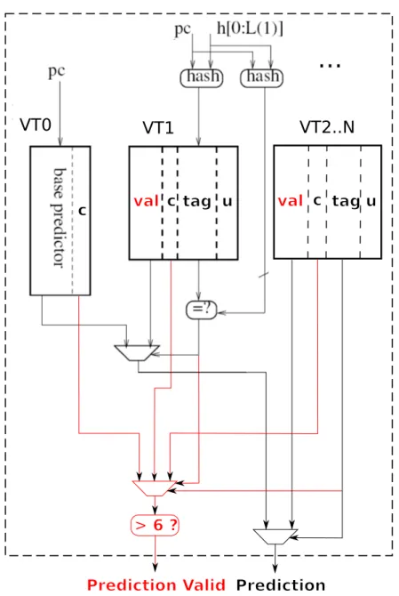
Figure 1: N-components VTAGE predictor. Val is the prediction, c is the hysteresis counter (acting as confidence counter), u is the useful bit used by the replacement policy to find an entry to evict.

Fig. 1 describes a N-component VTAGE predictor. It works similarly to the ITTAGE pre-dictor: all components are checked in parallel to find the provider and alternate components. Then, we check the confidence counter of the component actually making the prediction to see if it is saturated. If yes, we let the prediction proceed, otherwise, no prediction is made for the current instruction.

(10)

3.2 Prediction Latency is not an Issue on VTAGE

If VTAGE features large tables then the prediction latency can be quite high. However, prediction latency is not a major issue on VTAGE since the values are needed rather late in the pipeline (after register renaming stage). This has to be contrasted with conventional branch predictors, local value history predictors and stride value predictors. For branch predictors, we need the result of the prediction to predict the next branch. For the local history predictor, we need the (predicted or computed) results of the previous occurrences of the instruction to compute the prediction. The same goes for the stride predictors: they need the immediate previous value to compute the current prediction. On the contrary, VTAGE only needs the current branch history and should be much more resilient to delayed updates: By nature, it can predict without knowing the outcome of the previous instruction instance.

4 Maximizing Accuracy Through Confidence on Value

Pre-dictors

Predictor #Entries Tag _{Sat, Inc, Dec) Sat. Prob.}Conf(Thr, Rand filter B-hist Width

LVP [9] 4096 Full (52) (7, 7, 1, 7) 1/16

-2D-Str [4] 4096 Full (52) (7, 7, 1, 7) 1/16 -PS [11] _{1024 (4-way, VHT)}1024 (4-way, SHT) Full (54)_{Full (54)} (7, 7, 1, 7)_- 1/16_- 2 -o4-FCM 4096 (VHT) Full (52) (7, 7, 1, 7) 1/32

-[2, 15] 2048 (VPT) - - -

-VTAGE _6×1024 (Base)_{512 (T-comp)} _{10 + rank}- (7, 7, 1, 7) 1/32 -(7, 7, 1, 7) 1/32 11, 27, 642, 4, 6,

.

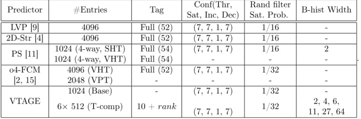
Table 1: Layout Summary. For VTAGE predictor, rank is the position of the tagged component and varies from 1 to 6.

We already mentioned in Section 2 that the performance cost of a value misprediction will be quite high. The effective misprediction penalty depends on the actual design implemented to handle the misprediction. Therefore, associating a confidence counter with each predictor entry is needed on every predictor. If one uses predictions only when the confidence counter is saturated then the accuracy will be in the 96-98% range for predictors such as LVP, FCM, the stride predictor or even VTAGE (see Section 6). However a 96-98% accuracy will not lead to a significant enough performance increase even with advanced selective replay for the mispredicted instruction and all the dependent instructions [19].

In [16], Seznec addressed the issue of isolating a class of very high level confidence branch predictions on the TAGE predictor. He showed that predictions provided by saturated counters are high confidence, but that it is possible to increase the level of confidence for this class by filtering the transition of the counter from nearly saturated to saturated using a random filter. On a correct prediction and if the providing counter is nearly saturated it is set to saturated only with a low probability (e.g. 1 out of 16 or 1 out of 1325). The transition from saturated to nearly saturated is always performed on a misprediction. This method allows to increase the prediction accuracy on the high level confidence prediction class at the cost of a decrease of its coverage. Riley et al. also considered some form of probabilistic counters in [12].

(11)

All the value predictors we consider in our evaluation have (or were added) confidence coun-ters, allowing to discriminate between high confidence and low confidence predictions. Saturated confidence counters correspond to high confidence predictions. In order to reinforce the accu-racy on high confidence predictions, we use the same random transition from nearly saturated to saturated as for the TAGE branch predictor. Moreover, the confidence counter is reset on a misprediction.

The results we present in Section 6 show that through applying such a simple modification to the predictor update automaton, value predictors are amenable to very high accuracy on high confidence predictions, but at the cost of decreasing the coverage of the predictors.

5 Evaluation Methodology

5.1 Test Suite

We gathered all results using PIN and the x86_64 ISA. As our test suite, we used all benchmarks from the SPEC’06 suite. We compiled the benchmarks using gcc3_{. We fed all benchmarks their}

respective reference workloads. Instrumentation begins with the 30Bth_{instruction and lasts until}

200 million instructions have been retired. Each component tries to predict all results (including floating point values) as well as effective addresses. Note that since a single instruction (hence PC) can lead to two predictions (address and result), we left-shift the PC by one and add either 0 or 1 to differentiate the two predictions when necessary. Furthermore, as PIN only exposes committed instructions, we assume that the predictors and branch histories are immediately updated.

The number of benchmarks is high (12 for SPEC’06INT and 17 for SPEC’06FP). Conse-quently, we only report cumulated results as well as results for a few of them, because several benchmarks behave in the same manner when it comes to Value Prediction. Specifically, we chose three integer benchmarks (perlbench, bzip2 and gobmk) and three floating point bench-marks (namd, soplex and lbm).

5.2 Value Predictors

5.2.1 Single Component Predictors

We study the behavior of several distinct value predictors in addition to the VTAGE predictor. On the one hand, three computational predictors in the form of the Last Value predictor [9], the 2-delta Stride predictor (2D-Str) [4] and the Per-Path Stride predictor [11]. On the other hand, a context-based predictors in the form of a generic order 4 FCM predictor (o4-FCM) [2, 15] as it outperformed the 2-level predictor (with a threshold of 12 so as to favor accuracy) of Wang et al. [18] in our experiments.

For this study we consider medium size predictors whose parameters are illustrated in Table 1. Each of these predictors necessitates about 256-512 Kbits of storage for implementation. We did not make any attempt to optimize the area of the predictors, e.g. full strides are used as well as full tags when relevant, so as to maximize accuracy. Therefore, the effective sizes should be viewed as an upper bound rather than an absolute requirement to achieve a given performance level. Indeed, it has been shown that partial strides cover most of what full strides can cover [13]. Similarly, full tags might not be a cost-effective way to maximize accuracy due to the presence of confidence estimation.

3_{gcc -O3 -mfpmath=sse -march=native -mtune=native -msse4.1 -mno-mmx -m64 (-O1 for perlbench). GCC}

(12)

0 10 20 30 40 50 60 70 80 90 100 LVP 2D-Str PS FCM VTAGE 90 91 92 93 94 95 96 97 98 99 100 Coverage Accuracy Predictor

400.perlbench - Single Predictors - General Purpose

Coverage Accuracy (a) 400.perlbench - w/o Filter

400.perlbench - Single Predictors - General Purpose

Coverage Accuracy (b) 400.perlbench - w/ Filter 0 10 20 30 40 50 60 70 80 90 100 LVP 2D-Str PS FCM VTAGE 90 91 92 93 94 95 96 97 98 99 100 Coverage Accuracy Predictor

401.bzip2 - Single Predictors - General Purpose

Coverage Accuracy (c) 401.bzip2 - w/o Filter

401.bzip2 - Single Predictors - General Purpose

Coverage Accuracy (d) 401.bzip2 - w/o Filter

445.gobmk - Single Predictors - General Purpose

Coverage Accuracy (e) 445.gobmk - w/o Filter

445.gobmk - Single Predictors - General Purpose

Coverage Accuracy (f) 445.gobmk - w/ Filter

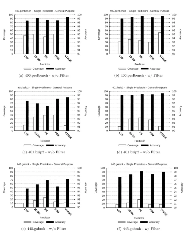
Figure 2: SPEC’06INT, general-purpose register prediction. Accuracy and coverage of distinct predictors with and without random saturation filtering.

(13)

average_int - Single Predictors - General Purpose

Coverage Accuracy (a) Average INT - w/o Filter

average_int - Single Predictors - General Purpose

Coverage Accuracy (b) Average INT - w/ Filter

Figure 3: SPEC’06INT average, general-purpose register prediction. Accuracy and coverage of distinct predictors with and without random saturation filtering.

As we have pointed out that accuracy is particularly important on value prediction, we simulated all predictors assuming a basic confidence counter mechanism, and we only use the predictions when the confidence counter is saturated. Table 1 describes the configurations of these confidence counters.

We simulated these predictor components with and without the random filter described in Section 4 so as to illustrate the loss of coverage that can be expected when aiming for such high accuracy. The probability used for the random filter was determined in order to achieve an accuracy of 99% or more for all components. The predictors can use a lower probability if even higher accuracy is needed. Adapting the probability at run-time, as suggested in [16], could also be considered.

5.2.2 Hybrid Predictors

We also focus on combination of several predictors - 2 and 3-component hybrids - so as to evaluate the potential of VTAGE to predict instructions not covered by any other prediction generation method. We do not consider all possible combinations as there would be too many, however, we retained the ones we found the most interesting.

First, for studying the complementarity of the components only, we will only consider the different sets of predictable results of each components among a given hybrid predictor. That is, we do not look and accuracy and coverage but only at the respective prediction sets of each components.

Nonetheless, to gain insight on what actual coverage can be expected, we apply a realistic selection mechanism to hybrid value predictors. Specifically, if only one component predicts, its prediction is naturally selected. When two or more predictors predict, the selection works as follows: use a majority vote if the three component predict and at least two provide the same result, do not predict if the three components disagree. Use a saturating 5-bit counter to monitor the respective efficiency of pairs of components to select among two predictions when there are only two components predicting. While very basic, this selection mechanism proved to be very effective in our simulations, in particular when we applied random filtering.

(14)

400.perlbench - Single Predictors - Address

Coverage Accuracy (a) 400.perlbench - w/o Filter

400.perlbench - Single Predictors - Address

Coverage Accuracy (b) 400.perlbench - w/ Filter 0 10 20 30 40 50 60 70 80 90 100 LVP 2D-Str PS FCM VTAGE 90 91 92 93 94 95 96 97 98 99 100 Coverage Accuracy Predictor

401.bzip2 - Single Predictors - Address

Coverage Accuracy (c) 401.bzip2 - w/o Filter

401.bzip2 - Single Predictors - Address

Coverage Accuracy (d) 401.bzip2 - w/ Filter 0 10 20 30 40 50 60 70 80 90 100 LVP 2D-Str PS FCM VTAGE 90 91 92 93 94 95 96 97 98 99 100 Coverage Accuracy Predictor

445.gobmk - Single Predictors - Address

Coverage Accuracy (e) 445.gobmk - w/o Filter

445.gobmk - Single Predictors - Address

Coverage Accuracy (f) 445.gobmk - w/ Filter

Figure 4: SPEC’06INT, address prediction. Accuracy and coverage of distinct predictors with and without random saturation filtering.

(15)

average_int - Single Predictors - Address

Coverage Accuracy (a) Average INT - w/o Filter

average_int - Single Predictors - Address

Coverage Accuracy (b) Average INT - w/ Filter

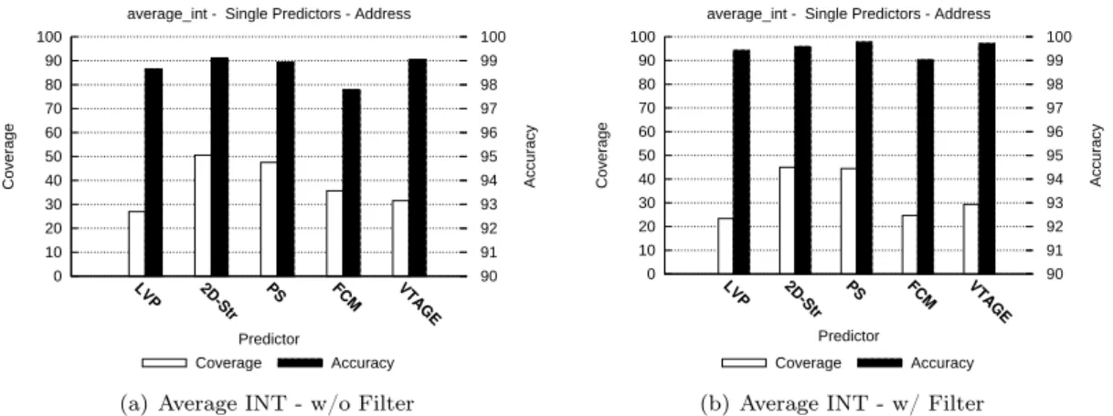
Figure 5: SPEC’06INT average, address prediction. Accuracy and coverage of distinct predictors with and without random saturation filtering.

5.3 Metrics

In this study, we only focus on the qualities of Value Prediction per se. Performance impact of Value Prediction is very dependent on many parameters such as the structure of the superscalar processor and the precise recovery mechanisms for mispredictions and will be addressed in future work. Therefore we will only display accuracy and coverage.

For each predictor, we collect the number of correct, incorrect and not predicted results and deduce accuracy and coverage. Accuracy is the amount of correct predictions out of the attempted predictions, i.e.:

Accuracy = correct (correct + incorrect)

Coverage is the amount of VP-eligible results the predictor is able to capture, i.e.: Coverage = correct

(VP-eligible results)

6 Simulation Results

In this section, we present results for three categories of instruction results, integer arithmetic, address computation and floating point operations.

6.1 Single Predictors

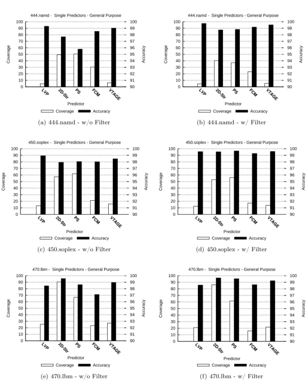
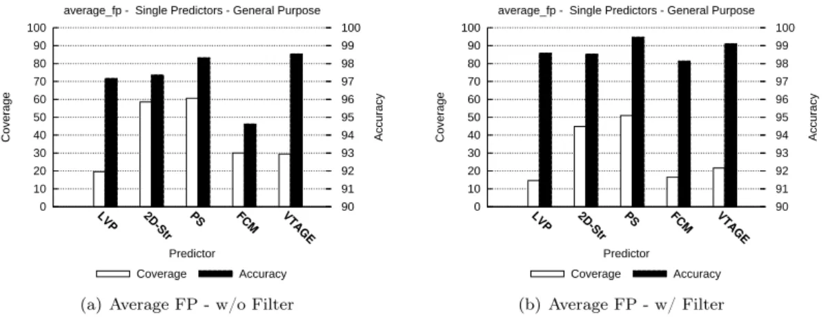
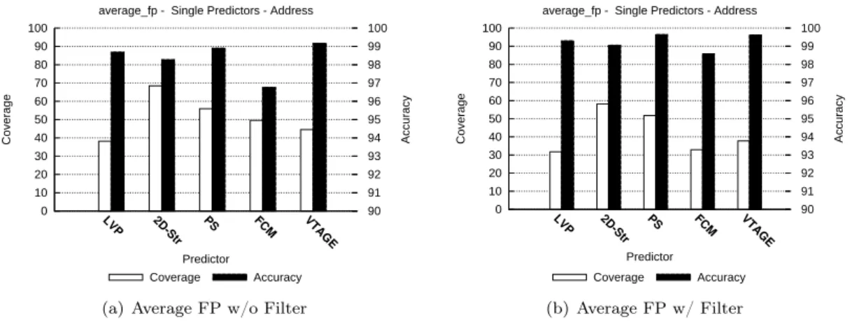
Figs. 2 through 9 respectively summarize the accuracy and coverage of the considered predictors with and without the random filter for some representative benchmarks of the SPEC’06INT and SPEC’06FP suite for general-purpose results and addresses. Figs. 10 and 11 summarizes them for floating point results on SPEC’06FP benchmarks. The bottom part of each figure illustrates the arithmetic mean obtained on either SPEC’06INT or SPEC’06FP.

(16)

444.namd - Single Predictors - General Purpose

Coverage Accuracy (a) 444.namd - w/o Filter

444.namd - Single Predictors - General Purpose

Coverage Accuracy (b) 444.namd - w/ Filter 0 10 20 30 40 50 60 70 80 90 100 LVP 2D-Str PS FCM VTAGE 90 91 92 93 94 95 96 97 98 99 100 Coverage Accuracy Predictor

450.soplex - Single Predictors - General Purpose

Coverage Accuracy (c) 450.soplex - w/o Filter

450.soplex - Single Predictors - General Purpose

Coverage Accuracy (d) 450.soplex - w/ Filter 0 10 20 30 40 50 60 70 80 90 100 LVP 2D-Str PS FCM VTAGE 90 91 92 93 94 95 96 97 98 99 100 Coverage Accuracy Predictor

470.lbm - Single Predictors - General Purpose

Coverage Accuracy (e) 470.lbm - w/o Filter

470.lbm - Single Predictors - General Purpose

Coverage Accuracy (f) 470.lbm - w/ Filter

Figure 6: SPEC’06FP, general-purpose register prediction. Accuracy and coverage of distinct predictors with and without random saturation filtering.

(17)

average_fp - Single Predictors - General Purpose

Coverage Accuracy (a) Average FP - w/o Filter

average_fp - Single Predictors - General Purpose

Coverage Accuracy (b) Average FP - w/ Filter

Figure 7: SPEC’06FP average, general-purpose register prediction. Accuracy and coverage of distinct predictors with and without random saturation filtering.

6.1.1 Without Random Filters

From Figs. 2 through 5, we can observe that integer computations are usually better predicted with stride-based predictors, except in the case of perlbench where VTAGE cover more predic-tions.

From Fig. 6 through 9, we can see that floating point benchmarks behave similarly to integer ones: stride-based predictors cover more results than context-based predictors: up to 30% more results on average for general-purpose results. This is understandable as the computation heavy part of those benchmarks is composed of floating point operations. Therefore, we expect the general-purpose computations to be more regular, hence predictable. This phenomenon is less pronounced on addresses but can still be observed. Accuracy is nearing 98% for LVP and PS but FCM lags behind at 95% for general-purpose results, on average.

The behavior of predictions of floating point values is also interesting. Context-based predic-tors appear as more efficient since coverage is slightly higher on average: 3 to 4% of the overall predictions. Accuracy is around 99% for computational predictors and 98% for context-based ones. However, some benchmark such as namd and lbm exhibit very little FP predictability. Also, note that due to the very nature of floating point values (three separate fields: sign, ex-ponent and mantissa), conventional stride-based predictors will lose efficiency if partial strides are used. This phenomenon does not appear here since we use strides of the same length as the prediction.

6.1.2 With Random Filters

The considered figures also show accuracy and coverage for the same benchmarks when adding the random filter to all predictors. We show the probabilities we used in Table 1. All predictors now feature an accuracy which is close to 99% on average on both SPEC’06INT and SPEC’06FP, at a cost of between 3 and 11% in coverage (2 to 3% for floating point values). FCM is the least precise although its accuracy is always greater than 98%. In general, the penalty in coverage is less pronounced for VTAGE than for FCM.

(18)

444.namd - Single Predictors - Address

Coverage Accuracy (a) 444.namd - w/o Filter

444.namd - Single Predictors - Address

450.soplex - Single Predictors - Address

Coverage Accuracy (c) 450.soplex - w/o Filter

450.soplex - Single Predictors - Address

Coverage Accuracy (d) 450.soplex - w/ Filter 0 10 20 30 40 50 60 70 80 90 100 LVP 2D-Str PS FCM VTAGE 90 91 92 93 94 95 96 97 98 99 100 Coverage Accuracy Predictor

470.lbm - Single Predictors - Address

Coverage Accuracy (e) 470.lbm - w/o Filter

470.lbm - Single Predictors - Address

Coverage Accuracy (f) 470.lbm - w/ Filter

Figure 8: SPEC’06FP, address prediction. Accuracy and coverage of distinct predictors with and without random saturation filtering.

(19)

average_fp - Single Predictors - Address

Coverage Accuracy (a) Average FP w/o Filter

average_fp - Single Predictors - Address

Coverage Accuracy (b) Average FP w/ Filter

Figure 9: SPEC’06FP average, address prediction. Accuracy and coverage of distinct predictors with and without random saturation filtering.

or recover some lost coverage but this choice is dependent on the misprediction recovery policy, among other design choices. Still, a probability of 1/32 is generally sufficient to near 99.5% accuracy for VTAGE when FCM will need to use a lower one (further decreasing its coverage) to reach that accuracy level on all prediction types. Adapting the probability at run-time could also be considered to achieve a predetermined level of accuracy as suggested in [16].

6.1.3 Summary

To summarize, we showed that given a random filter, all existing predictors including VTAGE are amenable to a very high accuracy, at a slight to noticeable cost in coverage. For the predictors size we considered, computational predictors are more storage-efficient except for floating point results where context-based predictors appear slightly more adapted. Previous work has already noted that for context-based predictors to beat computational predictor, bigger sizes need to be considered [14]. Given the supposed availability of a large number of transistors, using context-based predictors such as VTAGE is a direction to further explore. Moreover, using hybrid predictors is a simple way to increase coverage [15].

6.2 Hybrid Value Predictors

To achieve high coverage, hybridizing values predictors is necessary. To that extent, we present results for 2- and 3-component predictors using the random filter mechanism. Fig. 12 summa-rizes the amount of predictions exclusively captured by a given component in a specific hybrid, abstracting any selection mechanism. By lack of space, we only report numbers cumulated on the whole SPEC’06 suite and we consider all types of predictions (general-purpose, addresses and floating point). Therefore, rather than giving us insight on what speedup can be expected, these numbers reflect the predictability exposed by the overall suite to different prediction methods when they are combined.

We observe that hybrid predictors made of a context-based component and a stride-based component indeed show good complementarity, as expected [15]. The computational component is generally able to exclusively capture slightly more than two times more predictions than the

(20)

444.namd - Distinct Predictors - Floating Point

Coverage Accuracy (a) 444.namd - w/o filter

444.namd - Distinct Predictors - Floating Point

450.soplex - Distinct Predictors - Floating Point

Coverage Accuracy (c) 450.soplex - w/o filter

450.soplex - Distinct Predictors - Floating Point

Coverage Accuracy (d) 450.soplex - w/ filter 0 10 20 30 40 50 60 70 80 90 100 LVP 2D-Str PS FCM VTAGE 90 91 92 93 94 95 96 97 98 99 100 Coverage Accuracy Predictor

470.lbm - Distinct Predictors - Floating Point

Coverage Accuracy (e) 470.lbm - w/o filter

470.lbm - Distinct Predictors - Floating Point

Coverage Accuracy (f) 470.lbm - w/ filter

Figure 10: SPEC’06FP, floating point prediction. Accuracy and coverage of distinct predictors with and without random saturation filtering.

(21)

average_fp - Distinct Predictors - Floating Point

(a) Average FP - w/o filter

average_fp - Distinct Predictors - Floating Point

Coverage Accuracy (b) Average FP - w/ filter

Figure 11: SPEC’06FP average, floating point prediction. Accuracy and coverage of distinct predictors with and without random saturation filtering.

0 10 20 30 40 50 60 70 80 90 100

FCM+2D-Str VTAGE+2D-StrFCM+PS VTAGE+PS VTAGE+FCM 2D-Str+FCM+VTAGEPS+FCM+VTAGE

Percentage of Instrumented Instructions

average - Hybrids Summary

1st Correct Only 2nd Correct Only 3rd Correct Only Correct Shared Incorrect Not Predicted

Figure 12: Average complementarity of different hybrid components. SPEC’06, all predictions (general-purpose, addresses, FP).

(22)

0 10 20 30 40 50 60 70 80 90 100

2D-Str+FCM_w/o_filter2D-Str+FCM PS+FCM_w/o_filterPS+FCM 2D-Str+FCM+VTAGEPS+FCM+VTAGE 95

96 97 98 99 100 Coverage Accuracy

average - Hybrids Summary

Coverage Accuracy

Figure 13: Average accuracy and coverage of 2 and 3-component hybrid predictors using the selection mechanisms detailed in 5. A random filter is used for confidence except for bars labelled with _w/o_filter.

context-based component. The amount of predictions captured by both components is also close to the number of predictions exclusively captured by the computational component.

However, an interesting phenomenon is that the hybrid predictor made of two context-based components (namely FCM and VTAGE) also shows complementarity. Specifically, on average, VTAGE exclusively predicts 15.11% of the results, FCM 11.13% and both do predict another 15.66%. Recall that this is in fact the upper bound of the attainable coverage. This behavior implies that a 3-component hybrid featuring a computational component, FCM and VTAGE can yield an even better coverage.

The two rightmost bars of Fig. 12 describe the prediction sets of such 3-component hy-brids. Even though the sets of exclusively predictable results of the two context-based com-ponents are quite small, VTAGE can bring an additional coverage of respectively 7.02% (2D-Str+FCM+VTAGE) and 7.29% (PS+FCM+VTAGE). The computational component can once again exclusively predict more results (13.26% for 2D-Str and 16.22% for PS) while FCM lags be-hind at respectively 6.65% (2D-Str+FCM+VTAGE) and 6.98% (PS+FCM+VTAGE). Nonethe-less, there is potential for a 3-component hybrid featuring VTAGE.

To gauge what accuracy and coverage can be attained using a realistic selector, we ran the benchmark suite using the mechanism described in Section 5. For 3-component hybrid predictors, we use a majority vote selector and three 5-bit saturating counters. For 2-component hybrid predictors, we use a simple 5-bit saturating counter. Fig. 13 summarizes the numbers when considering such mechanisms. Specifically, we can attain 56.76% coverage and 99.48% accuracy with our 3-component PS+FCM+VTAGE when PS+FCM (resp. PS+FCM without filter) culminates at 49.83% (resp. 55.5%) coverage and 99.46% (resp. 98.62%) accuracy. In essence, VTAGE is able to bring back the coverage lost due to the addition of the random filter to the PS+FCM and 2D-Str+FCM predictors, while keeping the overall accuracy near 99.5%.

(23)

7 Key Directions for Future Work

Collecting accuracy and coverage of value predictors is not sufficient to assert the performance benefit. We need to Evaluate a value predictor in a realistic pipeline to gauge its effective impact. To that extent, our future work will focus on simulating the VTAGE predictor and its hybrid extensions, and assess the actual speedup they can yield. In order to do so, many possibilities exist regarding the implementation of Value Prediction. In this section, we discuss some of these possibilities.

7.1 Impact of Speculative Updates and Speculative History

Theoretically, the predictor can be accessed as soon as the instruction address is known, but the prediction can only be updated once the result is known, that is, several cycles after the fetch stage. From previous works in branch prediction [8], the impact on such delayed updates is known to be limited on the accuracy of the branch predictor, but might slightly impact the coverage of high confidence predictions. We have to verify that this property also stands for value predictors such as VTAGE.

In the case of context-based predictors using local history, however, speculative updates imply that each entry can contain a speculative history, with the associated overhead. Supporting speculative value history is a challenge in itself on a deep pipeline, especially when a single entry can be accessed several times before it is updated by a committed instruction. Coverage might also be affected by the following phenomenon: if one of the in-flight occurrences is low confidence then the speculative history is also low confidence. The two same phenomena potentially apply to stride-based predictors.

7.2 Prediction Criticality

Several studies make the observation that the speedup obtainable from Value Prediction is related with the number of critical results correctly predicted rather than with the predictor coverage [3, 5, 13]. For instance, previous studies have shown that predicting the result of load instructions is important [3, 10], especially as the gap between processor speed and memory speed is large. Calder et al. state that only predicting the result of load instructions can provide up to 75% of the potential speedup while only predicting 30% of the VP-eligible instructions [3].

The challenge is to identify critical instructions and/or critical instances of these instructions and to limit the use of predictions to these instructions. This might allow to determine which predictor component(s) should be favored in an effective implementation. Additionally, it might guide the choice of components in the predictor.

8 Conclusion

Even though Value Prediction has not been considered for current commercially available mi-croprocessors, the move toward heterogeneous architectures calls for very effective superscalar cores to quickly execute the sequential workloads. Given the availability of a large number of transistors, Value Prediction appears as a possibility to increase performance.

In this paper, we have made two contributions that may favor the introduction of value predictors in effective hardware.

First we have derived the Value TAGE predictor from the ITTAGE predictor by leveraging the similarities between Indirect Target Branch Prediction and Value Prediction. We have shown that the baseline VTAGE predictor is able to reach fairly high coverage and high accuracy, in the

(24)

range of what can be attained with existing predictors augmented with conventional confidence counters when necessary. Since VTAGE uses global branch history instead of per-instruction value history, it appears more easily implementable than other context-based predictor using local value history. Due to its structure, VTAGE should be much more efficient in a wide-issue, deeply pipelined superscalar processor because of its resiliency to speculative history and prediction latency: only the current branch history - which can be provided by the branch predictor - is required to predict and its prediction is needed very late. Consequently, incorporating VTAGE alone in a processor might prove to be a worthy tradeoff between coverage/accuracy and ease of implementation.

Second, we have shown that adding a random filter to force the confidence counters to saturate with a low probability is beneficial: A very high accuracy (> 99%) can be ensured for nearly all the value predictors at some cost in coverage. This cost is reasonable for VTAGE (always < 5%) but can reach roughly 10% for other predictors in some cases. Nonetheless, a very high accuracy is especially interesting since the performance benefit that can be expected from value prediction can be seriously impaired by the cost of mispredictions.

Furthermore, we have verified that computational and context-based predictors are comple-mentary to some extent. However, among context-based predictors, local value history-based and global branch history-based predictors exclusively predict a decent amount of results. This can be leveraged to increase prediction coverage.

As a consequence, we studied the possibility of using 3-component hybrid predictors composed of VTAGE, FCM and PS/2D-Str. We showed that using a very simple selector and the random filter to maximize accuracy, we can attain 56.76% coverage on average while maintaining 99.48% accuracy on SPEC2006 workload, when the PS+FCM has significantly less coverage (49.83%) for a similar accuracy (99.46%).

References

[1] G.M. Amdahl. Validity of the single processor approach to achieving large scale computing capabilities. In Proceedings of the spring joint computer conference, April 18-20, 1967., pages 483–485. ACM, 1967.

[2] M. Burtscher. Improving Context-Based Load Value Prediction. PhD thesis, University of Colorado, 2000.

[3] B. Calder, G. Reinman, and D.M. Tullsen. Selective value prediction. In Proceedings of the 26th International Symposium on Computer Architecture, 1999., pages 64–74. IEEE, 1999. [4] R.J. Eickemeyer and S. Vassiliadis. A load-instruction unit for pipelined processors. IBM

Journal of Research and Development, 37(4):547–564, 1993.

[5] J. González and A. González. The potential of data value speculation to boost ilp. In Proceedings of the 12th international conference on Supercomputing, pages 21–28. ACM, 1998.

[6] J.L. Hennessy and D.A. Patterson. Computer architecture: a quantitative approach. Morgan Kaufmann Pub, fifth edition, 2012.

[7] M.D. Hill and M.R. Marty. Amdahl’s law in the multicore era. Computer, 41(7):33–38, 2008.

(25)

[8] D.A. Jiménez. Reconsidering complex branch predictors. In Proceedings of the Ninth In-ternational Symposium on High-Performance Computer Architecture, 2003., pages 43–52. IEEE, 2003.

[9] M.H. Lipasti and J.P. Shen. Exceeding the dataflow limit via value prediction. In Proceedings of the 29th annual ACM/IEEE international symposium on Microarchitecture, pages 226– 237. IEEE Computer Society, 1996.

[10] M.H. Lipasti, C.B. Wilkerson, and J.P. Shen. Value locality and load value prediction. ASPLOS-VII, 1996.

[11] T. Nakra, R. Gupta, and M.L. Soffa. Global context-based value prediction. In Proceedings of the Fifth International Symposium On High-Performance Computer Architecture, 1999., pages 4–12. IEEE, 1999.

[12] Nicholas Riley and Craig B. Zilles. Probabilistic counter updates for predictor hysteresis and stratification. In HPCA, pages 110–120, 2006.

[13] B. Rychlik, J. Faistl, B. Krug, and J.P. Shen. Efficacy and performance impact of value prediction. In Proceedings of the International Conference on Parallel Architectures and Compilation Techniques, 1998., pages 148–154. IEEE, 1998.

[14] Y. Sazeides and J.E. Smith. Implementations of context based value predictors. Techni-cal report, Department of ElectriTechni-cal and Computer Engineering, University of Wisconsin-Madison.

[15] Y. Sazeides and J.E. Smith. The predictability of data values. In Proceedings of the 30th Annual IEEE/ACM International Symposium on Microarchitecture, 1997., pages 248–258. IEEE, 1997.

[16] A. Seznec. Storage free confidence estimation for the tage branch predictor. In Proceedings of the 17th International Symposium on High Performance Computer Architecture, 2011., pages 443–454. IEEE, 2011.

[17] A. Seznec and P. Michaud. A case for (partially) tagged geometric history length branch prediction. Journal of Instruction Level Parallelism, 8:1–23, 2006.

[18] K. Wang and M. Franklin. Highly accurate data value prediction using hybrid predictors. In Proceedings of the 30th annual ACM/IEEE international symposium on Microarchitecture, pages 281–290. IEEE Computer Society, 1997.

[19] H. Zhou, C. ying Fu, E. Rotenberg, and T. Conte. A study of value speculative execution and misspeculation recovery in superscalar microprocessors. Technical report, Department of Electrical & Computer Engineering, North Carolina State University, pp.–23, 2000.

(26)

Campus universitaire de Beaulieu