HAL Id: hal-00362625
https://hal.archives-ouvertes.fr/hal-00362625
Submitted on 19 Feb 2009
HAL is a multi-disciplinary open access
archive for the deposit and dissemination of
sci-entific research documents, whether they are
pub-lished or not. The documents may come from
teaching and research institutions in France or
abroad, or from public or private research centers.
L’archive ouverte pluridisciplinaire HAL, est
destinée au dépôt et à la diffusion de documents
scientifiques de niveau recherche, publiés ou non,
émanant des établissements d’enseignement et de
recherche français ou étrangers, des laboratoires
publics ou privés.
Estimation of the Absolute Orientation of a Five-link
Walking Robot with Passive Feet
Yannick Aoustin, Gaëtan Garcia, Philippe Lemoine
To cite this version:
Yannick Aoustin, Gaëtan Garcia, Philippe Lemoine. Estimation of the Absolute Orientation of a
Five-link Walking Robot with Passive Feet. Armando Carlos de Pina Filho. Humanoid Robots:
New Developments, I-Tech Education and Publishing, Vienna, Austria, Chap. 3, pp. 31-44, 2007,
Advanced Robotic Systems, 978-3-902613-00-4. �hal-00362625�
Estimation of the Absolute Orientation of a
Five-link Walking Robot with Passive Feet.
Yannick Aoustin, Gaëtan Garcia, Philippe Lemoine
Institut de Recherche en Communications et Cybernétique de Nantes (IRCCyN),
École Centrale de Nantes, Université de Nantes, U.M.R. 6597, 1 rue de la Noë,
BP 92101, 44321 Nantes Cedex 3, France.
e-mail: surname.name@irccyn.ec-nantes.fr
1. Introduction
One of the main objectives of current research on walking robots is to make their gaits more fluid by introducing imbalance phases. For example, for walking robots without actuated ankles, which are under actuated in single support, dynamically stable walking gaits have been designed with success (Aoustin & Formal’sky 2003; Chevallereau et al. 2003; Zonfrilli et al. 2002; Aoustin et al. 2006; Pratt et al. 2001; Westervelt et al.). Both the design of reference motions and trajectories and the control of the mechanism along these trajectories usually require the knowledge of the whole state of the robot. This state contains internal variables which are easy to measure using encoders for example, and also the absolute orientation of the robot with respect to the horizontal plane. For robots with unilateral constraints with the ground, it may not be possible to derive the latter information from internal measurements, as in the case of the absolute orientation of a biped in single support. Of course, technological solutions exist such as accelerometers, gyrometers, inertial units… But the implementation of these solutions is expensive and difficult.
In order to overcome these difficulties, we propose to use a state observer which, based on the measurements of the joint variables and on a dynamic model of the robot, provides estimates of the absolute orientation of the walking robot during imbalance phases. This strategy was first validated in simulation for a three link biped without feet, using nonlinear high gain observers and a nonlinear observer based on sliding modes with a finite time convergence (Lebastard et al. 2006a) and (Lebastard et al. 2006b), for walking gaits composed of single support phases and impacts. The main drawback with this family of observers is that, when only some of the degrees of freedom are measured, a state coordinates transformation is necessary to design their canonical form (Gauthier & Bornard 1981; Krener & Respondek 1985; Bornard & Hammouri 1991; Plestan & Glumineau 1997).
In this chapter, the observer is an extended Kalman filter and it is applied to
SemiQuad,
a prototype walking robot built at our institute. SemiQuad is a five link mechanism with a platform and two double-link legs. It is designed to study quadruped gaits where both front legs (resp. rear legs) have identical movements. Its unique front leg (resp. rear leg) acts as the two front legs (resp. rear legs) of the quadruped, so that SemiQuad can be considered as an implementation of a virtualquadruped, hence its name
.
The legs have passive (uncontrolled) feet that extend in the frontal plane. Due to this, the robot is stable in the frontal plane. Four motors located in haunches and knees drive the mechanism. The locomotion of the prototype is a planar curvet gait. In double support, our prototype is statically stable and over actuated. In single support, it is unstable and under actuated.The reference walking gaits have been designed using an intuitive strategy which is such that the absolute orientation is not required. Still, it contains imbalance phases during which the observer can be used, and its results evaluated. The estimation results being correct, such an observer can be used for contexts where the absolute angle is necessary. Furthermore, the idea can be useful for other types of walking robots, such as bipeds with imbalance phases.
The organization of this chapter is the following. Section 2 is devoted to the model of
SemiQuad. It also contains the data of its physical parameters. The intuitive gaits which were
designed for SemiQuad are presented in section 3. The statement of the problem of estimation of the absolute orientation of SemiQuad is defined in Section 4. Simulation results and experimental results avec presented in section 5. Section 6 presents our conclusions and perspectives.
2. Presentation and dynamic models of SemiQuad
2.1 SemiQuad
The prototype (see figure 1) is composed of a platform and two identical double-link legs with knees. The legs have passive (uncontrolled) feet that extend in the frontal plane. Thus, the robot can only execute 2D motions in the sagittal plane, as considered here. There are four electrical DC motors with gearbox reducers to actuate the haunch joints between the platform and the thighs and the knee joints. Using a dynamic simulation, we have chosen parameters of the prototype (the sizes, masses, inertia moments of the links) and convenient actuators. The parameters of the four actuators with their gearbox reducers are specified in Table 1. The lengths, masses and inertia moments of each link of SemiQuad are specified in Table 2.
DC motor
+gearbox length (m) mass (kg) gearbox ratio Rotor inertia (kg.m2)
Electromagnetical torque constant (N.m)/A in haunch In knee 0.23 0.23 2.82 2.82 50 50 3.25 10-5 2.26 10-5 0.114 0.086 Table 1. Parameters of actuators
physical parameters of each link mass (kg) length (m) Center of mass locations (m) Moment of inertia (kg
.
m2)around the center of mass Ci (I=1,…,5)
links 1 and 5: shin link 3: platform +actuators in each haunch
links 2 and 4: thigh +actuators in each knee
m1 = m5 = 0.40 m3 = 6.618 m2 = m4 = 3.21 l1 = l5 = 0.15 l3 = 0.375 l2 = l4=0.15 s1 = s5 = 0.083 s3 = 0.1875 s2 = s4 = 0.139 I1 = I5 = 0.0034 I3 = 0.3157 I2 = I4 = 0.0043
Table 2. Parameters of SemiQuad
The maximum value of the torque in the output shaft of each motor gearbox is 40 N
.
m . This saturation on the torques is taken into account to design the control law in simulation and in experiments. The total mass of the quadruped is approximately 14 kg. The four actuated joints of the robot are each equipped with one encoder to measure the angular position. The angular velocities are calculated using the angular positions. Currently the absolute platform orientation angleα
(see figure 2) is not measured. As explained before, the proposed walking gait does not require this measurement. Each encoder has 2000 pts/rev and is attached directly to the motor shaft. The bandwidth of each joint of the robot is determined by the transfer function of the mechanical power train (motors, gearboxes) and the motor amplifiers that drive each motor. In the case of SemiQuad, we have approximately a 16 Hz bandwidth in the mechanical part of the joints and approximately 1.7 kHz for the amplifiers. The control computations are performed with a sample period of 5 ms (200 Hz). The software is developped in C language.Fig. 2. SemiQuad’s diagram: generalized coordinates, torques, forces applied to the leg tips, locations of mass centers.
2.2 Dynamic model of SemiQuad
Figure 2 gives the notations of the torques, the ground reactions, the joint variables and the Cartesian position of the platform. Using the equations of Lagrange, the dynamic model of
SemiQuad can be written:
+ + = Γ + 1 + 2 e e e e e e R 1 R 2 D q&& H q& G B D R D R (1) with, ⎡ ⎤ = ⎢⎣ ⎥⎦ T T : e p p
q q x z . The vector q is composed of the joint actuated variables and the absolute orientation of the platform, = ⎢⎡ ⎤
⎥
⎣ ⎦
T
: 1 2 3 4
q θ θ θ θ α ;
(
x ,z are the Cartesian p p)
coordinates of the platform center. The joint angle variables are positive for counter clockwise motion. D (q)e
(
7 7 is the inertia positive definite matrix. The matrix ×)
e
H (q,q)&
(
7 7 represents the Coriolis and centrifugal forces and ×)
G (q)e(
7 1×)
is the vectorof the gravity forces. Be is a constant matrix composed of ones and zeros. Each matrix
j R
D (q)(7 2× ) ( j =1,2 ) is a jacobian matrix which represents the relation between feet Cartesian velocities and angular velocities. It allows to take into account the ground reaction
j
R on each foot. If foot j is not in contact with the ground, then Rj= ⎣⎡0,0 . The ⎤⎦T
term = ⎢⎡ ⎤ ⎥
⎣ ⎦
Γ Γ Γ Γ Γ T
: 1 2 3 4 is the vector of four actuator torques. Let us assume that during
the single support, the stance leg acts as a pivot joint. Our hypothesis is that the contact of the swing leg with the ground results in no rebound and no slipping of the swing leg. Then, in single support, equation (1) can be simplified and rewritten as:
+ + = Γ
Dq Hq G B&& & (2) As the kinetic energy =K 1q DqT
2& & does not depend on the choice of the absolute frame (see (Spong, M. & Vidyasagar M. 1991)) and furthermore variable α defines the absolute orientation of SemiQuad, the inertia matrix D
(
5 5×)
does not depend on α , and then D D θ θ θ θ . As =(
1, 2, 3, 4)
for the case of equation (1), the matrix H(q,q)&
(
5 5×)
represents the Coriolis and centrifugal forces and G(q)(
5 1×)
is the vector of gravity forces. B is a constant matrix composed of ones and zeros. Equation (2) can be written under the following state form:(
Γ)
= + Γ⎡
⎤
⎢
⎥
⎣
-1⎦
rel q x = f(x) g(q ) D -Dq - G + B & & & (3)With x= ⎣⎡qT q&T⎤⎦Tand the joint angle vector ⎡ ⎤
= ⎢⎣ ⎥⎦
T
1 2 3 4
rel
q θ θ θ θ . The state space is defined as ∈ ⊂ 10=
{
=⎣⎡ T &T⎦⎤T & <& < ∞ ∈ −π π]
]
5}
M
x X R x q q q q ; q , . From these definitions, it is clear that all state coordinates are bounded.
2.3 Discrete Model
Our objective is to design an extended Kalman filter with a sampling period ∆ to observe the absolute orientation α . Then it is necessary to find a discrete model equivalent to (3). A possible solution is to write ≈ + −
∆
k 1 k
x x
= + ∆ + Γ
k+1 k k relk k
x x (f(x ) g(q ) ) (4)
For SemiQuad, we have preferred to sample the generalized coordinates and their velocities using approximations to a different order by a Taylor development:
∆ ∆ ∆2x(t)+ + ∆nx (t)n + x(t + ) = x(t) + x(t) + ... ε
2! n! &&
& , (5)
From (5), developments to second order and first order have been used for the generalized coordinates and their velocities, respectively. Limiting the order where possible limits the noise, but using second order developments for position variables introduces their second order derivative and allows to make use of the dynamic model.
2 k 1 k k k 5 1 k 1 k k q q q q q q q 2 0 + × + ⎛ ⎞ ⎛≈ ⎞+ ∆⎛ ⎞+∆ ⎛ ⎞ ⎜ ⎟ ⎜ ⎟ ⎜ ⎟ ⎜ ⎟ ⎝ ⎠ ⎝ ⎠ ⎝ ⎠ ⎝ ⎠ & &&
& & && (6)
With this method, a discrete model of (3) is calculated. If we add the equation corresponding to the measurement of the joint angles, we obtain the following system:
(
)
1 1 2 3 4 4 4 + = Γ = = θ θ θ θ = = s k k k T x k k k x f (x , ) y h(x ) Cx with C I (7)2.4 Impulsive impact equation
The impact occurs at the end of the imbalance phase, when the swing leg tip touches the ground, i.e. :
{
f}
x S∈ = x X q=q∈ where q is the final configuration of SemiQuad. The instant of impact f
is denoted by T . Let us use the index 2 for the swing leg, and 1 for the stance leg during the i
imbalance phase in single support. We assume that: ♦ the impact is passive, absolutely inelastic;
♦ the swing leg does not slip when it touches the ground; ♦ the previous stance leg does not take off;
♦ the configuration of the robot does not change at the instant of impact.
Given these conditions, at the instant of an impact, the contact can be considered as impulsive forces and defined by Dirac delta-functions Rj=IRj∆ −(t T )i (j=1, 2). Here
j Nj Tj
T
R R R
I = ⎣⎡I I ⎤⎦ , is the vector of the magnitudes of the impulsive reaction in leg j (Formal’sky 1974). The impact model is calculated by integrating (1) between Ti−(just before
impact) and Ti+(just after impact) . The torques provided by the actuators at the joints, and
Coriolis and gravity forces, have finite values, thus they do not influence the impact. Consequently the impact equation can be written in the following matrix form:
(
)
1 1 2 2e e e R R R R
D (q) q&+−q− =D (q)I +D (q)I (8) Here, q is the configuration of SemiQuad at t T= , i q& and e− q& are the angular velocities just e+
before and just after impact, respectively. Furthermore, the velocity of the stance leg tip before impact is null. Then we have:
1 02 1 T R e D q+ × = & (9)
After impact, both legs are stance legs, and the velocity of their tip becomes null:
1 2 4 1 0 T R e T R D q D + × ⎛ ⎞ = ⎜ ⎟ ⎜ ⎟ ⎝ ⎠& (10)
3. Walking gait strategy for SemiQuad
By analogy with animal gaits with no flight phase, SemiQuad must jump with front or back leg to realize a walking gait. There is no other way to avoid leg sliding. Then it is necessary to take into account that SemiQuad is under actuated in single support and over actuated in double support. Let us briefly present the adopted strategy to realize a walking gait for SemiQuad. It was tested first in simulation to study its feasibility and then experimentally (Aoustin et al. 2006). A video can be found on the web page
http://www.irccyn.ec-nantes.fr/irccyn/d/en/equipes/Robotique/Themes/Mobile. Figure 4 represents a sequence of stick configurations for one step to illustrate the gait. Let us consider half step n as the current half step, which is composed of a double support, a single support on the rear leg and an impact on the ground. During the double support, SemiQuad has only three degrees of freedom. Then its movement can be completely prescribed with the four actuators. A reference movement is chosen to transfer the platform centre backwards. This is done by defining a polynomial of third order for both Cartesian coordinates xp and zp. The coefficients of these polynomials are
calculated from a choice of initial and final positions, of the initial velocity and an intermediate position of the platform centre. The reference trajectories for the four actuated joint variables are calculated with an inverse geometric model. Then, by folding and immediately thrusting the front leg, the single support phase on the rear leg starts. During this imbalance phase,
SemiQuad has five degrees of freedom and its rotation is free around its stance leg tip in the sagittal plane. Reference trajectories are specified with third order polynomial functions in time for the four actuated inter-link angles. However, the final time Tp of these polynomial
functions is chosen smaller than the calculated duration Tss of the single support phase, such
that before impact the four desired inter-link angles(θ i = 1,...,4) become constant. Using this id
strategy, we obtain the desired final configuration of our prototype before the impact even if Tss is not equal to the expected value.
= + + + = θ ≤ ≤ 2 3 0 1 2 3 p id ie p p ss id θ a a t a t a t if t < T θ (T ) if T t T (11) The coefficients of these polynomials are calculated from a choice of initial, intermediate
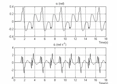
and final configurations and of the initial velocity for each joint link. Just after impact, the next half step begins and a similar strategy is applied (figure 4). The tracking of the reference trajectories is achieved using a PD controller. The gains, which were adjusted using pole placement, were tested in simulation and in experiments. Figure 3 shows the evolutions of the absolute orientation variable α(t) and its velocity α(t)& , obtained from the simulation of SemiQuad for five steps. These graphs clearly show that the dynamics of the absolute orientation cannot be neglected in the design of a control law based on a state feedback. The durations of the double support phase and the single support phase are 1.5 s and 0.4 s respectively.
Fig. 3. Evolution of α(t) and α(t)& in simulation during the walking gait for five steps.
4. Observation of the absolute orientation of SemiQuad
System (3) is generically observable if the following matrix O has a full rank (see (Plestan & Glumineau 1997)), which is equal to 10, with ( k ,...,k )1 p the p observability indexes.
(
− −)
Ο = k1 1 kp 1
1 f 1 p f p
dh ... dL h ... dh ... dL h (12) where dh is the gradient vector of function h (see system (7)) with respect to the state vector
x, and dLfh is the Lie derivative of h along the vector field f. We have also checked that the
equivalent property is satisfied by the discrete model. This means that, at each sampling time tk, it is possible to find an observability matrix with 10 independent rows or columns.
Having checked system observability, we propose an Extended Kalman Filter to observe the absolute orientation. The design of this Extended Kalman Filter is now described.
In practice, due to uncertainty in the determination of parameters and to angular measurement errors, system (3), and of course system (7), are only approximations. A standard solution is to represent modelling and measurement errors as additive noises disturbing the system.
Let us consider the associated ``noisy’’ system:
(
)
1 + = Γ + α = = + β s k k k k T 1 2 3 4 k k k x f (x , ) y C(x ) θ θ θ θ (13)In the case of a linear system, if αkand βk are white Gaussian noises, mutually
independent and independent of x, the Kalman filter is an optimal estimator. When the system is not linear, it is possible to use the Extended Kalman Filter (EKF) by linearizing the evolution equation fs and the observation equation (which is in our case linear) around the
interest and the effectiveness of the Extended Kalman Filter have been proved in many experimental cases. The EKF is very often used as a state observer (Bonnifait & Garcia 1998).
(a) Double support (half step n) : The projection of the platform center
is halfway between the leg tips
(f) Double support (end of half step n and start of half step n+1): Just after landing with an impact of the front leg. After half step
n, the platform center has moved forward.
(b) Double support (half step n) : The projection of the platform center is
closer to the back leg tip
(g) Double support (half step n+1) : The projection of the platform center is
closer to the front leg tip.
(c) Double support (half step n): The front leg is unbent just before take off (before the single support)
(h) Double support (half step n+1): The back leg is unbent just before take off
(before the next single support phase)
(d) Single support (half step n): Just after jump of the front leg,
the front leg is bent.
(i) Single support (half step n+1) : Just after jump of the back leg,
the back leg is bent.
(e) Single support (half step n): The distance between the leg tips
is larger than in the previous double support phase.
(j) Single support (half step n+1): The distance between the leg tips is smaller than
in the previous double support phase.
Fig. 4. Plot of half steps n and n+1 of SemiQuad. as a sequence of stick figures. In the case of our system, the equations of the EKF are:
1 1 − + − α + = Γ = + s k k k T k k k k x f (x , ) P A P A Q ) ) (14)
• a posteriori estimation: uses data available at tk+1
(
)
(
)
1 1 1 1 1 10 10 1 1 1 − − + + + + + − × + + + = + − = − k k k k k k k k x x K y Cx P I K C P ) ) (15) with: = ∂ ⎛ ⎞ = ⎜∂ ⎟ ⎝ ⎠ k s k x x f A x ) and(
)
− − − β + = + + + 1 T T k 1 k 1 k 1 K P C CP C QHere yk+1 are the measured joint variables, which are the first four components of vector xk
at time tk, and Cx)k+1- is the a priori estimation of these joint variables. Q and α Q are the β
covariance matrices of αkand βk, K is the Kalman gain and P the estimated covariance
matrix of prediction ( -P at tk) and estimation ( P at tk) errors.
5. Simulation and experimental results.
For the simulation and experimental tests, the physical parameters defined in section 2 are used. The sampling period ∆ is equal to 5 ms. The incremental encoders having N=2000 points per revolution, the variance of measurement is taken equal to π2
(
3∆N2)
=8.225 10-4.The errors of incremental encoders being independent, we have chosen Q =8.225 10β -4 I4 4× .
The components of Qαfor the configuration variables are determined by trial and error
from simulation and experimental results. The components of Qαfor velocity variables are
derived from the values for position variables, taking into account the sampling period, and are larger than those corresponding to position variables.
− − ⎛ ⎞ = ⎜ ⎟ ⎝ ⎠ 10 5x5 5x5 α 5 5x5 5x5 3.0 10 I 0 Q 0 3.0 10 I
The initialization of the covariance matrix P takes into account a determination of α less precise and fixes the variances on the velocities, as for Qα, taking into account of the sampling period.
− ⎛ ⎞ ⎜ ⎟ = ⎜ ⎟ ⎜ ⎟ ⎝ ⎠ 10 4x4 4x1 4x5 -5 0 1x4 1x5 -2 5x4 5x1 5x5 8 10 I 0 0 P 0 1.7 10 0 0 0 5 10 I
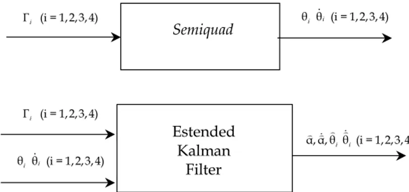
All the tests in simulations and in experiments were done following the scheme of figure 5. In simulations, the joint variables θiand their velocities θ& (i=1,2,3,4) obtained by integration of i
the direct dynamic model of SemiQuad and the control torques Γi (i=1,2,3 4) are the inputs of
the Extended Kalman Filter. For the experimental tests, the joint variables θi (i=1,2,3 4) are
measured and differentiated to obtain the velocities θ& . These eight variables, together with i
the four experimental torques Γ (i=1,2,3,4) are the inputs of the Extended Kalman Filter. In i
Semiquad
i Γ (i = 1,2,3, 4)Estended
Kalman
Filter
i i . θ θ (i = 1,2,3,4) i Γ (i = 1,2,3, 4) i i ) ) ) )& & α, α, θ θ (i = 1,2,3,4) i i . θ θ (i = 1,2,3,4)Fig. 5. Principle of tests of the Extended Kalman Filter with SemiQuad.
5.1 Simulation results
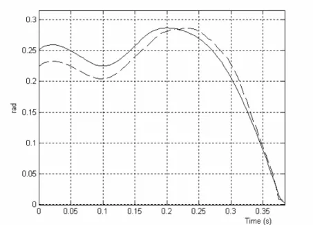
Figure 6 shows the evolution of the estimated and real orientations of the platform during a single support phase of the cyclic walking gait of SemiQuad. The initial error, which has been set to 0.0262 rad (1.5 degree), is rapidly reduced, andthe estimated orientation converges towards the real orientation. Let us notice that a maximum value of 1.5 degree for the initial error is reasonable because experimentally α(0)) is determined by the geometric model at the end of the previous double support.
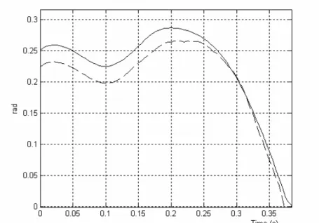
In the model used by the observer, we do not consider any friction. We have performed robustness tests of our estimator by adding a viscous friction, Γ =i F θv i
(i=1,2,3,4), and a Coulomb friction Γ =i F θ& (i=1,2,3,4) to the simulation model. Figure s i
7 shows the estimated and real orientations of the platform of SemiQuad in the case when a viscous friction is added. The coefficient Fv equals to 0.1 N.m.s/rad. Similarly,
figure 8 shows the estimated and the real orientations of the platform of SemiQuad in the case of a Coulomb friction, with a coefficient Fs equal to 0.2 N.m. Last robustness
test (figure 9) presents the estimated and real orientations of the platform of
SemiQuad with an inertia reduced by 5% for the platform in the simulator. In practice, 5% precision on inertia is feasible (see identification results in (Lydoire & Poignet 2003)).
From these robustness tests, we can conclude that we have no finite time convergence. However, the final relative errors of the estimated orientations of the platform of SemiQuad are small. Since it will be possible to update the initial condition of the estimator during the next double support phase, with the measurements of the encoders and the geometrical relations, such errors are not a problem.
5.2 Experimental results
At each step, the estimator is initialized with the configurations and the velocities at the end of the previous double support phase. At each sampling time, velocities are obtained by the usual differentiation operation = i − i −
i
θ (k∆) θ ((k 1)∆) θ
∆
& (i=1,2,3 4). No filtering is
applied to smooth the measured joint variables θi, their velocities θ& and the four torques i i
Fig. 6. Absolute orientation α(t) of the platform: real (solid) and estimated (dashed).
Fig. 7. Absolute orientation α(t) of the platform: real (solid) and estimated (dashed), with a supplement viscous friction.
Fig. 8. Absolute orientation α(t) of the platform: real (solid) and estimated (dashed), with a supplement Coulomb friction.
Fig. 9. Absolute orientation α(t) of the platform: real (solid) and estimated (dashed), with an error on the inertia of the platform.
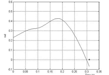
Figure 10 shows the estimation of the absolute orientation of the platform α(t) . The duration of the single support phase is 15% smaller than in simulation. It can probably be explained by the fact that our knowledge of the physical parameters of the robot is not perfect, and that we neglected effects such as friction in the joints.
Currently, there is no experimental measured data about the evolution of α(t) in single support, because SemiQuad is not equipped with a sensor such as a gyrometer or a gyroscope. However, in double support, using the geometric and kinematic models it is possible to calculate α(t) and α(t)& . In addition to providing initial conditions for the observer, this also allows to calculate the orientation at the end of the single support phase, just after impact. The corresponding value is displayed as a star on the next graph, and is equal to 0.01 rad (0.57 degree). The difference between this value and the estimated value at the same instant is almost 3 degrees.
Fig. 10. Estimation of the absolute orientation α(t) of the platform using the experimental data.
6. Conclusion
An application of the digital Extended Kalman Filter has been presented for the problem of estimating the absolute orientation of SemiQuad, a 2D dynamically stable walking robot. There are some differences between simulations and experiments, but the results still prove the ability of our observer to yield a short term estimation of the orientation of the robot. The precision is sufficient for the estimation to be useful for calculating the dynamic model and monitoring the balance of the robot. This task is important for SemiQuad, and vital for bipeds, to which the idea is also applicable (see Lebastard, Aoustin, & Plestan 2006 for a different type of observer). Given the possibility to re-initialize the observer at each double support phase, even if very short, as it can be for bipeds, the observer can provide the absolute orientation over time without the use of any additional sensor, which was the goal of our work.
In a near future, we plan to equip SemiQuad with a gyrometer to fully evaluate the performance of our estimator over time. Our perspective is to use the estimated orientation in advanced feedback controllers.
7. References
Aoustin, Y. & Formal’sky, A. (2003). Control design for a biped: Reference trajectory based on driven angles as function of the undriven angle, Journal of Computer and System
Sciences International, Vol. 42, No. 4, (July-August 2003) 159-176.
Chevallereau, C.; Abba, G.; Aoustin, Y.; Plestan, F. ; Westervelt, E. R.; Canudas de Wit, C. & Grizzle, J. W. (2003). Rabbit: A testbed for advanced control theory, IEEE Control
Systems Magazine, Vol. 23, (October 2003) No. 5, 57-78.
Zonfrilli, F.; Oriolo, M. & Nardi, T. (2002). A biped locomotion strategy for the quadruped robot Sony ers-210, Proceedings of IEEE Conference on Robotics and Automation, pp. 2768-2774.
Aoustin, Y.; Chevallereau, C. & Formal’sky, A. (2006). Numerical and experimental study of the virtual quadruped-SemiQuad, Multibody System Dynamics, Vol. 16, 1-20. Pratt, J.; Chew, C. M.; Torres, A.; Dilworth, P. & Pratt, G. (2001). Virtual model control: an
intuitive approach for bipedal locomotion, International Journal of Robotics Research, Vol. 20, No. 2, 129-143.
Westervelt, E. R.; Grizzle, J. W. & Koditschek, D. E. (2003). Hybrid zero dynamics of planar biped walkers, IEEE Transactions on Automatic Control, Vol. 48, No. 1, (February 2003) 42-56. Lebastard, V.; Aoustin, Y. & Plestan, F. (2006). Observer-based control of a walking biped
robot without orientation measurement, Robotica, Vol. 24, 385-400.
Lebastard, V.; Aoustin, Y. & Plestan F. (2006) . Absolute orientation estimation for observer-based control of a five-link biped robot, Springer Verlag Series Notes on Control and
Information Sciences, Editor: K. Kozlowski, Springer, vol. 335, Lecture Notes in Control and Information Sciences, 2006.
Gauthier, J.P. & Bornard, G. (1981). Observability for any u(t) of a class of nonlinear system.
IEEE Transactions on Automatic Control, 26(4): 922-926.
Krener, A. & Respondek, W. (1985). Nonlinear observers with linearization error dynamics,
SIAM Journal Control Optimization, Vol. 2, 197-216.
Bornard, G. & Hammouri, H. (1991). A high gain observer for a class of uniformly observable systems, Proceedings of the 30th IEEE Conference on Decision and Control,
pp. 1494-1496.
Plestan, F. & Glumineau, A. (1997). Linearisation by generalized input-ouput injection,
Systems and Control Letters, Vol. 31, 115-128.
Spong, M. & Vidyasagar M. (1991). Robot dynamics and control, John Wiley, New-York. Formal’sky, A. M. (1982). Locomotion of Anthropomorphic Mechanisms, Nauka, Moscow [In
Russian], 368 pages.
Bonnifait, P. & Garcia, G. (1998). Design and experimental validation of an odometric and goniometric localization system for outdoor robot vehicles, IEEE Transactions on
Robotics and Automation, Vol. 14, No. 541-548.
Lydoire, F. & Poignet, Ph. (2003). Experimental dynamic parameters identification of a seven dof walking robot, Proceedings of the CLAWAR’03 Conferencel, pp. 477-484.