HAL Id: tel-01761768
https://hal.archives-ouvertes.fr/tel-01761768
Submitted on 9 Apr 2018HAL is a multi-disciplinary open access archive for the deposit and dissemination of sci-entific research documents, whether they are pub-lished or not. The documents may come from teaching and research institutions in France or abroad, or from public or private research centers.
L’archive ouverte pluridisciplinaire HAL, est destinée au dépôt et à la diffusion de documents scientifiques de niveau recherche, publiés ou non, émanant des établissements d’enseignement et de recherche français ou étrangers, des laboratoires publics ou privés.
Romain Brault
To cite this version:
Romain Brault. Large-scale operator-valued kernel regression. Machine Learning [cs.LG]. Université Paris Saclay, 2017. English. �NNT : 2017SACLE024�. �tel-01761768�
16, 2017 s u p e rv i s o r:
Professor (Prof.) Florence d’Alché-Buc l o c at i o n:
46, Rue Barrault, 75013 — Paris, France d i g i ta ly s i g n e d d o c u m e n t:
gpg --keyserver keys.gnupg.net \
--recv-keys A276D73294A106E2544FFF9E3E5B5D0B181C5E04 gpg --verify ThesisRomainBrault.pdf.asc ThesisRomainBrault.pdf
In this thesis we study scalable methods to perform regression with Operator-Valued Kernelsin order to learn vector-valued functions.
When data present structure, or relations between them or their different components, a common approach is to treat the data as a vector living in an appropriate Hilbert space rather than a collec-tion of real numbers. This representacollec-tion allows to take into account the structure of the data by defining an appropriate space embbed-ing the underlyembbed-ing structure. Thus many problems in machine learn-ing can be cast into learnlearn-ing vector-valued functions. Operator-Valued Kernels and vector-valued Reproducing Kernel Hilbert Spaces provide a theoretical and practical framework to address the issue of learn-ing vector-valued functions by naturally extendlearn-ing the well-known framework of scalar-valued kernels. In the context of scalar-valued functions learning, a scalar-valued kernel can be seen a similarity measure between two data points. A solution of the learning prob-lem has the form of a linear combination of theses similarities with respect to weights (to determine), in order to have the best “fit” of the data. When dealing with Operator-Valued Kernels, the evaluation of the kernel is no longer a scalar similarity, but a function (an operator) acting on vectors. A solution is then a linear combination of operators with respect to vector weights.
Although Operator-Valued Kernels generalize strictly scalar-valued kernels, large scale applications are usually not affordable with these tools that require an important computational power along with a large memory capacity. In this thesis, we propose and study scalable methods to perform regression with Operator-Valued Kernels. To achieve this goal, we extend Random Fourier Features, an approx-imation technique originally introduced for scalar-valued kernels, to Operator-Valued Kernels. The idea is to take advantage of an approxi-mated operator-valued feature map in order to come up with a linear model in a finite dimensional space.
First we develop a general framework devoted to the approxima-tion of shift-invariant Mercer kernels on Locally Compact Abelian groups and study their properties along with the complexity of the algorithms based on them. Second we show theoretical guarantees by bounding the error due to the approximation, with high probability. Third, we study various applications of Operator Random Fourier Features to different tasks of Machine learning such as multi-class
framework with other state of the art methods. Fourth, we conclude by drawing short-term and mid-term perspectives.
q
and with sufficient computational speed to make use of machine-learning techniques, but our knowledge of the basic principles of these techniques is still rudimentary. Lacking such knowledge, it is necessary to specify methods of problem solution in minute and exact detail, a time-consuming and costly procedure. Programming computers to learn from experience should eventually eliminate the need for much of this detailed programming effort.” — Arthur Samuel [145]
A C K N O W L E D G E M E N T S
First of all I would like to express my sincere gratitude to my advisor Prof. Florence d’Alché-Buc for guiding me, the continuous support during this Ph. D thesis and her insightful remarks.
Besides my advisor, I would also like to thank my thesis jury Prof. Liva Ralaivola and Prof. Paul Honeine for their time.
This thesis would not have been possible without my collaborators Dr. Markus Heinonen and Dr. Maxime Sangnier, whose help have been precious to develop fully my ideas and publish. I would like to thank Dr. Nicolas Goix, Dr. Nicolas Drougard and Maël Chiapino with whom it has been a pleasure to collaborate on a paper. Big thank to Alexandre Gramfort for helping me through the deployment of operalib in the context of the misssion Paris-Saclay Center for Data Science.
I would also like to acknowledge the Université d’Évry-val-d’Essonne for hosting and funding1 me for the first part of my thesis and Télécom ParisTech for the second part.
This manuscript is dedicated to my parents and family for backing me up during this three years and especially my grand parents for welcoming me any week-end to their place to rest.
I am also thankful to all my colleagues at Evry: Néhémy Lim, Yves-Stan Le Cornec, Adel Mezime, Sebastien Maurais, Vincent Chau, Céline Brouard, Arnaud Fouchet, Frédéric Papadopoulos, Markus Heinonen, Laurent Poligny and Jean-Baptiste Meuniere and also
1 PhD grant numbered 76391.
Maël Chiapino, Ana Korba, Albert Thomas, Adil Salim and Jean La-font for the great conversations at work as well as the pub!
q
i i n t ro du c t i o n 1
1 outline and motivations 3
1.1 Motivation . . . 4
1.2 Outline . . . 4
2 on learning efficently scalar-valued functions 7 2.1 About statistical learning . . . 8
2.1.1 Introduction to kernel methods . . . 11
2.1.2 Towards large scale learning with kernels . . . . 14
3 background 21 3.1 Notations . . . 22
3.1.1 Algebraic structures . . . 22
3.1.2 Topology and continuity . . . 22
3.1.3 Measure theory . . . 23
3.1.4 Vector spaces, linear operators and matrices . . 24
3.2 Elements of abstract harmonic analysis . . . 26
3.2.1 Locally compact Abelian groups . . . 26
3.2.2 The Haar measure . . . 29
3.2.3 Even and odd functions . . . 30
3.2.4 Characters . . . 30
3.2.5 The Fourier Transform . . . 33
3.2.6 Representations of Groups . . . 35
3.3 On Operator-Valued Kernels . . . 36
3.3.1 Definitions and properties . . . 36
3.3.2 Shift-Invariant OVK on LCA groups . . . 43
3.3.3 Examples of Operator-Valued Kernels . . . 44
3.3.4 Some use of Operator-valued kernels . . . 48
ii c o n t r i b u t i o n s 51 4 operator-valued random fourier features 53 4.1 Motivation . . . 54
4.2 Theoretical study . . . 54
4.2.1 Sufficient conditions of existence . . . 56
4.2.2 Examples of spectral decomposition . . . 62
4.2.3 Functional Fourier feature map . . . 67
4.3 Operator-valued Random Fourier Features . . . 69
4.3.1 Building Operator-valued Random Fourier Fea-tures . . . 69
4.3.2 From Operator Random Fourier Feature maps to OVKs . . . 72
4.3.3 Examples of Operator Random Fourier Feature maps . . . 75
4.3.4 Regularization property . . . 78
4.4 Conclusions . . . 80
5 bounding the error of the orff approximation 81 5.1 Convergence with high probability of the ORFF estimator 82 5.1.1 Random Fourier Features in the scalar case and decomposable OVK . . . 84
5.1.2 Uniform convergence of ORFF approximation on LCA groups . . . 85
5.1.3 Dealing with infinite dimensional operators . . 90
5.1.4 Variance of the ORFF approximation . . . 91
5.1.5 Application on decomposable, curl-free and divergence-free OVK . . . 93
5.2 Conclusions . . . 94
6 learning with feature maps 95 6.1 Learning with OVK . . . 96
6.1.1 Supervised learning within VV-RKHS . . . 96
6.1.2 Learning with Operator Random Fourier Fea-ture maps . . . 100
6.2 Solving ORFF-based regression . . . 103
6.2.1 Gradient descent methods . . . 103
6.2.2 Complexity analysis . . . 108
6.3 Efficient learning with ORFF . . . 109
6.3.1 Case of study: the decosubmposable kernel . . 110
6.3.2 Linear operators in matrix form . . . 113
6.3.3 Curl-free kernel . . . 116
6.3.4 Divergence-free kernel . . . 117
6.4 Experiments . . . 117
6.4.1 Learning with ORFF vs learning with OVK . . 117
6.5 Conclusion . . . 123
7 consistency and generalization bound for orff 125 7.1 Generalization bound . . . 126
7.1.1 Generalization by bounding the function space complexity . . . 127
7.1.2 Algorithm stability . . . 130
7.2 Consistency of learning with ORFF . . . 131
7.3 Discussion . . . 135
8 application to time series modelling 137 8.1 Introduction . . . 138
8.2 Operator-Valued Kernels for Vector Autoregression . . 138
8.3 Operator-Valued Random Fourier Features . . . 141
8.3.1 Numerical Performance . . . 143
8.3.2 Simulated data . . . 143
8.3.3 Influence of the number of random features . . 144
8.3.4 Real datasets . . . 145
iii c o n c l u s i o n a n d w o r k i n p ro g r e s s 147
9 work in progress 149
9.1 Learning function-valued functions . . . 150
9.1.1 Quantile regression . . . 150
9.1.2 Functional output data . . . 151
9.1.3 ORFF for functional output data . . . 151
9.1.4 Many quantile regression . . . 155
9.1.5 One-class SVM revisited . . . 157 9.2 Operalib . . . 160 10 conclusion 163 10.1 Contributions . . . 164 10.2 Perspectives . . . 165 iv a p p e n d i x 167 a p ro o f s o f t h e o r e m s 169 a.1 Proof of the error bound with high probability of the ORFF estimator . . . 170
a.1.1 Epsilon-net . . . 170
a.1.2 Bounding the Lipschitz constant . . . 171
a.1.3 Bounding the error on a given anchor point . . 172
a.1.4 Union Bound and examples . . . 176
a.2 Proof of the ORFF estimator variance bound . . . 181
b m i s c e l l a n e o u s 183 b.1 Learning with semi-supervision . . . 184
b.1.1 Representer theorem and feature equivalence . 184 b.1.2 Gradients . . . 189
b.1.3 Complexity . . . 191
c r e l e va n t p i e c e o f c o d e 195 c.1 Python code for figure 3.1 . . . 196
c.2 Python code for figure 5.1 . . . 197
c.3 Python code for figure 5.3 . . . 199
c.4 Python code for figure 5.4 . . . 201
c.5 Python code for figure 5.5 . . . 204
c.6 Python (tensorflow) code for continuous quantile re-gression . . . 207
d o n e c l a s s s p l i t t i n g c r i t e r i a f o r r a n d o m f o r e s t s 211 d.1 Background on decision trees . . . 215
d.2 Adaptation to the one-class setting . . . 216
d.2.1 One-class splitting criterion . . . 216
d.2.2 Prediction: scoring function of the forest . . . . 220
d.2.3 OneClassRF: a Generic One-Class Random For-est algorithm . . . 221
d.3 Benchmarks . . . 222
d.3.1 Default parameters of OneClassRF . . . 222
d.3.2 Results . . . 222
d.4.1 Underlying model . . . 224
d.4.2 Adaptive approach . . . 226
d.5 Conclusion . . . 227
d.6 Further insights on the algorithm . . . 228
d.6.1 Interpretation of parameter gamma . . . 228
d.6.2 Alternative scoring functions . . . 228
d.6.3 Alternative stopping criteria . . . 229
d.6.4 Variable importance . . . 229
d.7 Hyper-parameters of tested algorithms . . . 229
d.8 Description of the datasets . . . 231
d.9 Further details on benchmarks and outlier detection re-sults . . . 232
Figure 2.1 Borel’s strong law of large numbers. . . 10
Figure 2.2 Separation of nested circles with linear classifier 11 Figure 2.3 A scalar-valued feature map . . . 15
Figure 3.1 Riesz map, dual spaces and adjoints. . . 25
Figure 3.2 Synthetic 2D curl-free field . . . 46
Figure 3.3 Synthetic 2D divergence-free field . . . 47
Figure 4.1 Relationships between feature-maps. . . 68
Figure 4.2 Approximation of a function in a vv-RKHS us-ing different realizations of Operator Random Fourier Feature . . . 72
Figure 5.1 ORFF reconstruction error . . . 82
Figure 5.2 decomposable ORFF variance bound . . . 92
Figure 5.3 Curl-free ORFF variance bound . . . 92
Figure 6.1 ORFF equivalence theorem. . . 104
Figure 6.2 ORFF equivalence theorem with overfitting. . . 105
Figure 6.3 Efficient decomposable Gaussian ORFF . . . . 116
Figure 6.4 Efficient curl-free Gaussian ORFF . . . 116
Figure 6.5 Efficient divergence-free Gaussian ORFF . . . . 117
Figure 6.6 Prediction Error in percent on the MNIST dataset versus D, the number of Fourier fea-tures . . . 119
Figure 6.7 Empirical comparison between curl-free ORFF, curl-free OVK, independent ORFF, indepen-dent OVK on a synthetic vector field regression task. . . 120
Figure 6.8 Decomposable kernel on the third dataset: R2 score vs number of data in the train set (N) . 121 Figure 6.9 Decomposable kernel on the third dataset: R2 score vs number of data in the train set (N) for different number for different number of random samples (D). . . 122
Figure 9.1 Learning a continuous quantile function with ORFF regression. . . 152
Figure 9.2 Learning many quantile with joint OVK re-gression. . . 153
Figure 9.3 Learning a continuous quantile function with ORFF regression. . . 156
Figure 9.4 Continuous OCSVM: proportion of inlier with respect to nu . . . 159
Figure 9.5 Continuous OCSVM for outlier detection . . . 161
Figure B.1 ORFF equivalence theorem (semi-supervised) 190
Figure B.2 ORFF multiclass semi-supervised . . . 194
Figure D.1 Outliers distribution G in the naive and adap-tive approach. . . 216
Figure D.2 Adaptative splitting criteria . . . 218
Figure D.3 One Class Random Forest level-sets . . . 220
Figure D.4 Illustration of the standard splitting criterion on two modes when the proportion γ varies. . 230
Figure D.5 Performances of the novelety detection algo-rithms . . . 232
Figure D.6 Performances of the outlier detection algorithms233
Figure D.7 ROC and PR curves for OneClassRF (novelty detection framework) . . . 234
Figure D.8 ROC and PR curves for OneClassRF (outlier detection framework) . . . 234
Figure D.9 ROC and PR curves for IForest (novelty de-tection framework) . . . 234
Figure D.10 ROC and PR curves for IForest (outlier detec-tion framework) . . . 235
Figure D.11 ROC and PR curves for OCRFsampling (nov-elty detection framework) . . . 235
Figure D.12 ROC and PR curves for OCRFsampling (out-lier detection framework) . . . 235
Figure D.13 ROC and PR curves for OCSM (novelty detec-tion framework) . . . 236
Figure D.14 ROC and PR curves for OCSM (outlier detec-tion framework) . . . 236
Figure D.15 ROC and PR curves for LOF (novelty detection framework) . . . 236
Figure D.16 ROC and PR curves for LOF (outlier detection framework) . . . 237
Figure D.17 ROC and PR curves for Orca (novelty detection framework) . . . 237
Figure D.18 ROC and PR curves for Orca (outlier detection framework) . . . 237
Figure D.19 ROC and PR curves for LSAD (novelty detec-tion framework) . . . 238
Figure D.20 ROC and PR curves for LSAD (outlier detec-tion framework) . . . 238
Figure D.21 ROC and PR curves for RFC (novelty detection framework) . . . 238
Figure D.22 ROC and PR curves for RFC (outlier detection framework) . . . 239
Table 3.1 Mathematical symbols and their signification (part 1). . . 27
Table 3.3 Mathematical symbols and their signification (part 2). . . 28
Table 3.5 Classification of Fourier Transforms in terms of their domain and transform domain. . . 33
Table 6.1 Efficient linear-operators for different ORFF. . 112
Table 6.3 Time complexity of efficient linear-operators for different ORFF. . . 115
Table 6.5 Error (% of nMSE) on SARCOS dataset. . . 123
Table 8.1 Sequential SCV-MSE and computation times for VAR(1), ORFFVAR and OKVAR on syn-thetic data (Settings 1, 2 and 3). . . 144
Table 8.2 SVC-MSE with respect to D the number of ran-dom features for ORFFVAR. . . 145
Table 8.3 SCV-MSE and computation times for ORFF-VAR, VAR(1) and OKVAR on real datasets. . . 146
Table D.1 Original datasets characteristics . . . 221
Table D.3 Results for the novelty detection setting. . . . 223
Table D.4 Results for the outlier detection setting . . . . 240
ACML Asian Conference in Machine Learning
AUC Area Under the Curve
c. f. confer
cum. cumulative
ECML European Conference in Machine Learning
e. g. exempli gratia
FT Fourier Transform
i. e. id est
IForest Isolation Forest
i. i. d. independent identically distributed
KDD The Assotiation for Computing Machinery’s Spe-tial Interest Group on Knowledge Discovery and Data Mining
L-BFGS-B Limited-memory BroydenFletcherGoldfarb-Shanno algorithm for Bound constraind opti-mization
LCA Locally Compact Abelian
LOF Local Outlier Factor
LSAD Least Squares Anomaly Detection
MGF Moment Generating Function
N. A. Not Available
NORMA Naive Online regularized Risk Minimization Al-gorithm
OCRFsampling One-Class Random Forest Sampling OCSM One-Class Support Vector Machine
OKVAR Operator-Valued Kernel-Based Vector Autore-gressive
OneClassRF One-Class Random Forest
ONORMA Operator-valued Naive Online regularized Risk Minimization Algorithm
ORFF Operator-valued Random Fourier Feature ORFFVAR Operator-valued Random Fourier Feature Vector
Autoregressive
OVK Operator-Valued Kernel
PD Positive definite
p. d. f probibility density function
POVM Positive Operator-Valued Measure
PR Precision Recall
PSD Positive Semi-definite
RF Random Forest
RFC Random Forest Clustering
RFF Random Fourier Feature
RKHS Reproducing Kernel Hilbert Space ROC Receiver Operating Characteristic
r. v. random variable
SCV Sequential cross-validation
SCV-MSE Sequential cross-validation Mean Squared Error SPSD Symmetric Positive Semi-definite
SVM Support Vector Machine
UCI University of California Irvine
VAR Vector Autoregressive
VC-dimension Vapnik-Chernonenkis dimension
VV-RKHS Vector Valued Reproducing Kernel Hilbert Spa-ce
w. r. t. with respect to q
1
O U T L I N E A N D M O T I VAT I O N SIn this chapter we present our motivations as well as the structure of the present manuscript.
Contents
1.1 Motivation . . . 4 1.2 Outline . . . 4
1.1 motivation
This thesis is dedicated to the definition of a general and flexible approach to learn vector-valued functions together with an efficient implementation of the learning algorithms. To achieve this goal, we study shallow architectures, namely the product of a (nonlinear) operator-valued feature eΦ(x) and a parameter vector θ such that e
f(x) = eΦ(x)∗θ, and combine two appealing methodologies: Operator-Valued Kernel Regression and Random Fourier Features.
Operator-Valued Kernels [5, 34, 41, 84, 113] extend the classic scalar-valued kernels to functions with values in some output Hil-bert space. As in the scalar case, Operator-Valued Kernels (OVKs) are used to build Reproducing Kernel Hilbert Spaces (RKHS) in which representer theorems apply as for ridge regression or other appro-priate loss functional. In these cases, learning a model in the RKHS boils down to learning a function of the form f(x) =∑N
i=1K(x, xi)αi where x1, . . . , xN are the training input data and each αi, i= 1, . . . , N is a vector of the output space Y, and each K(x, xi) is an operator on vectors of Y.
However, OVKs suffer from the same drawbacks as classic (scalar-valued) kernel machines: they scale poorly to large datasets because they are exceedingly demanding in terms of memory and computa-tions. We propose to approximate OVKs by extending a methodology called Random Fourier Features (RFFs) [12,94,139,144,164,167,191] so far developed to speed up scalar-valued kernel machines. The RFF approach linearizes a shift-invariant kernel model by generating ex-plicitly an approximated feature map ˜φ. RFFs has been shown to be efficient on large datasets and has been further improved by effi-cient matrix computations such as [94, “FastFood”] and [61, “SORF”], which are considered as the best large scale implementations of ker-nel methods, along with Nyström approaches proposed in Drineas and Mahoney [55]. Moreover thanks to RFFs, kernel methods have been proved to be competitive with deep architectures [51,108,192]. 1.2 outline
Chapter 2. In this introductory chapter we recall some elements of the statistical learning theory started by Vapnik [177]. Then we recall kernel methods [9] which are used to construct spaces of scalar-valued functions (called RKHSs) that are used model and learn non linear dependencies from the data. We finish by a literature review on large-scale implementations of kernel methods based on random Fourier features [139] and the Nyström method [185].
Chapter 3. In this chapter, to conclude the introduction, we de-velop briefly the mathematical tools used throughout this manuscript. We give a full table of notations, and present elements of functional analysis [93] and abstract harmonic analysis [65]. Then we turn our attention to the case where the functions we want to learn are not real-valued, but vector-valued. To learn vector-valued functions we define Operator-Valued Kernels [41, 113] that generalize the scalar-valued kernel presented inChapter 2. We conclude by giving a non-exhaustive list of Operator-Valued Kernels along with the context in which they have been used.
Chapter 4. In this first contribution chapter we present a general-ization of the RFF framework introduced in Chapter 2 [29]. This is based on an operator-valued Bochner theorem proposed by Carmeli et al. [41]. We use this theorem to show how to construct an Operator-valued Random Fourier Feature (ORFF) from an OVK. Conversely we also show that it is possible to construct an ORFF from the regulariza-tion properties it induces rather than from an OVK. We give various examples of ORFF maps such as an ORFF map for the decomposable kernel, the curl-free kernel and the divergence-free kernel.
Chapter 5. In this contribution chapter we refine the bound on the OVK approximation with ORFF we first proposed in [29] and presented in [28]. It generalizes the proof technique of Rahimi and Recht [139] to OVK on LCA groups thanks to the recent results of Koltchinskii [92], Minsker [121], Sutherland and Schneider [167], and Tropp [175]. As a Bernstein bound it depends on the variance of the estimator for which we derive an “upper bound”.
Chapter 6. This contribution chapter focus on explaining how to define an efficient implementation and algorithm to train an ORFF model. First we recall the supervised ridge regression with OVK and the celebrated representer theorem [182]. Then we show under which conditions learning with an ORFF is equivalent to learn with a ker-nel approximation. Eventually we give the gradient for the ridge re-gression problem, useful to find an optimal solution with gradient descent algorithms, as well as a closed form algorithm. We conclude by showing how viewing ORFFs as linear operators rather than ma-trices yields a more efficient implementation and finish with some numerical applications on toy and real-world datasets.
Chapter 7. This contribution chapter deals with a generalization bound for the a regression problem with ORFF based on the results of Maurer [112] and Rahimi and Recht [140]. We also discuss the case of Ridge regression presented inChapter 6.
Chapter 8. This contribution chapter shows how to use the ORFF methodology for non-linear vector autoregression. It is an instanti-ation of the ORFF framework to X = Y = (Rd,+). We also give a generalization of a stochastic gradient descent [51] to ORFF. This is a joint work with Néhémy Lim and Florence d’Alché-Buc and has been published at a workshop of ECML. It is based on the previous work of Lim et al. [101] for time series vector autoregression with operator-valued kernels [30].
Chapter 9. To conclude our work we present some work in progress. We show practical applications of operator-valued kernels acting on an infinite dimensional space Y. We give two examples. First we show how to generalize many quantile regression to learn a con-tinuous function of the quantiles on the data. Second we apply the same methodology to the One-Class Support Vector Machine (OCSM) algorithm in order to learn a continuous function of all the level sets. We conclude by presenting Operalib, a python library developed dur-ing this thesis which aims at implementdur-ing OVK-based algorithms in the spirit of Scikit-learn [132].
2
O N L E A R N I N G E F F I C E N T LY S C A L A R - VA L U E D F U N C T I O N S“For such a model there is no need to ask the question “Is the model true?”. If “truth” is to be the “whole truth” the answer must be “No”. The only question of interest is “Is the model illuminating and useful?””. — George Box [27]
In this chapter we recall some elements of the statistical learning the-ory started by Vapnik [177]. Then we recall kernel methods [9] which are used to construct spaces of real-valued functions (called RKHS) that are used model and learn non linear dependencies from the data. We finish by a litterature review on large-scale implementation of ker-nel methods based on random Fourier features [139] and the Nyström method [185].
Contents
2.1 About statistical learning . . . 8 2.1.1 Introduction to kernel methods . . . 11
2.1.2 Towards large scale learning with kernels . 14
2.1 about statistical learning
We focus on the context of supervised learning. Supervised learn-ing aims at buildlearn-ing a function that predicts an output from a given input, by exploiting a “training set” composed of pairs of observed inputs/outputs. Denote X, an input space and Y, the output space. In this chapter, Y ⊆ R. When Y = { 1, . . . , C }, we talk about supervised classification. When Y = R, supervised learning corresponds to usual regression. We are given an independent identically distributed (i. i. d.) sample of size N of traning data s = (xi, yi)Ni=1, drawn from an un-known but fixed joint probability law Pr. We call learning algorithm, a function A that takes a class of functions F, a training sample s and re-turns a function in F. The learning algorithm can be studied through many angles, from a computational point of view to a statistical point of view.
From a limited number of observations, we wish to build a func-tion that captures the relafunc-tionship between the two random variables Xand Y. More specifically, we search for a function f in some class of functions, denoted F and called the hypothesis class such that the f ∈ F makes good predictions for the pair (X, Y) distributed accord-ing Pr. To convert this abstract goal into a mathematical definition, we define a local loss function L : X × F × Y → R+ that evaluates the capacity of a function f to predict the outcome y from an input x.
Hence, the goal of supervised learning is to find a function f ∈ F that minimizes the following criterion, called the true risk associated to L:
R (f)= EPr[L(X, f, Y)], (2.1)
using the training dataset. However, this definition comes with an im-portant issue: we do not know Pr(X, Y) and thus we cannot compute this risk nor minimize it. A first proposition is to replace this true risk by its empirical counterpart, the empirical risk, i. e. the empirical mean of the loss computed on the training data:
Remp (f, s) = 1 N N ∑ i=1 L(xi, f, yi).
Since the training data are usually supposed to be i. i. d., the cele-brated strong law of large numbers tells us that for any given function fin F, the empirical risk converges almost surely to the true risk.
Intuitively the empirical risk measures the performance of a model on the training data, while the true risk measures the performance of a model with respect to all the possible experiments (even the ones that are not present in the training set). Although the convergence of
the empirical risk to the true risk is guaranteed by the strong law of large numbers, for a given value of N, the function produced by min-imization of the empirical risk may suffer from overfitting, i. e. being too much adapted to the training data and having a poor behavior on new unseen data.
Generalization error bounds, first introduced by the seminal work of Vapnik [178] in the context of supervised binary classification and then largely studied in wider contexts (see for instance, Mohri, Ros-tamizadeh, and Talwalkar [122]), provide a tool to understand how the difference between the true risk and the empirical risk behaves given N, the size of the sample used to compute the empirical risk, and d, a measure of the capacity the hypothesis class. These bounds usually take the following form. For any δ ∈ (0, 1), with probability 1 − δ, the following holds for any function f ∈ F of capacity |F| ∈ R:
R(f) ⩽ Remp (f, s) + C(δ, N, |F|)
Especially for the functions of interest fsreturned by a learning algo-rithm, we have
R(fs) ⩽ Remp (fs, s) + C(δ, N, |F|).
Usually it is expected from the quantity C(δ, N, |F|) to increase with the capacity of the class of functions |F|, and to decrease when the number of points N increases. This suggests to control the complexity of the hypothesis class while minimizing the empirical risk. In other words, is the class of functions F is not too big, we expect that a low empirical risk implies a low true risk in particular when the number of training points N is large. Also when δ goes to zero, it is expected for C(δ, N, |F|) to go to infinity since 1 − δ is the probability of the bound to be valid1.
Most of the approaches in machine learning, and specifically in su-pervised learning, are based on regularizing approaches: in this case, learning algorithms minimize the empirical loss while controlling a penality term on the model f. In Subsection 2.1.1, we will choose an hypothesis class as an Hilbert space where the penalty can be ex-pressed as the ℓ2norm in this Hilbert space.
There is a crucial difference between the strong law of large num-bers and the generalization property of a learning algorithm. The strong law of large numbers holds after a model f has been selected and fixed in F. Thus minimizing the empirical risk does not yield ipso facto a model that minimizes the true risk (which measures the adequation of the model on unseen data). This can be illustrated by an intuitive example adapted from Cornuéjols and Miclet [47, page 64] and the infinite monkey theorem.
Figure 2.1: Borel’s strong law of large numbers.
Example 2.1 Suppose we have a recruiter (a learning algorithm) whose task is to select the best students from a pool of candidates (the class of functions). Given ten students the recruiter makes them pass a test with N questions. If the exam is well constructed and there are enough questions the recruiter should be able to retrieve the best student.
Now suppose that ten million monkeys ≫ N take the test and answer randomly to the questions. Then with high probability a monkey will score better or as well as the best student (strong law of large numbers). Can we say then that the recruiter has identified the best student?
Intuitively we see that when the capacity of the class of function grows (the number of students and random monkeys), the performance of the best element a posteriori (minimizing the empirical risk) is not linked to the future performance (minimizing the true risk). In the present example we see that the capacity of the class of function is too large with respect to the number of data and thus presents a risk of overfitting.
On the contrary the generalization property ensures that the difference between the empirical risk and the true risk is controlled because the bound does not depend on a single fixed model, but on the whole class of functions. In this case if there are too many random monkeys, C(δ, N, |F|) will blow-up, resulting in a poor generalization property.
A slightly stronger requirement is the consistency of learning algo-rithm. Given a loss function L and a class of function F there exists a optimal solutions that minimize the true risk.
f∗ ∈ arg min f∈F
R(f) .
The excess risk is defined as the difference between the empirical risk of a model returned by a learning algorithm and f∗. A learning algorithm is said to be consistent when it is possible to bound the excess risk uniformly over all the solutions returned by a learning algorithm.
be Positive Semi-definite (PSD) if for any (x1, . . . , xN) ∈ XN, the (Gram) matrix
K =(k(xi, xj)
)i=N,j=N
i=1,j=1 ∈ MN,N(R) is Symmetric Positive Semi-definite (SPSD)2.
The following proposition gives necessary and sufficient conditions to obtain a SPSD matrix:
Proposition 2.1 (SPSD matrix). K is SPSD if and only if it is symmetric and one of the following assertions holds:
• The eigenvalues of K are non-negative
• for any column vector c= (c1, . . . , cN)T∈ MN,1(R), cTKc =
N ∑ i,j=1
ciKijcj⩾0
One of the most important property of PD kernels [122] is that a PD kernel defines a unique RKHS. Note that the converse is also true. Theorem 2.1 (Aronszajn [9]). Suppose k is a symmetric, positive definite kernel on a set X. Then there is a unique Hilbert space of functions H on X for which k is a reproducing kernel, i. e.
(2.2a) ∀x ∈ X, k(·, x) ∈ H
(2.2b) ∀h ∈ H, ∀x ∈ X, h(x) = ⟨h, k(·, x)⟩H.
His called a reproducing kernel Hilbert space (Reproducing Kernel Hilbert Space) associated to k, and will be denoted, Hk.
Another way to use Aronszajn’s results is to state the feature map property for the PSD kernels.
Proposition 2.2 (Feature map). Suppose k is a symmetric, positive defi-nite kernel on a set X. Then, there exists a Hilbert space H and a mapping φfrom X to H such that:
∀x, x′ ∈ X, k(x, x′) = ⟨φ(x), φ(x′)⟩ H.
The mapping φ is called afeature map and H, a feature space.
Remark 2.1 Aronszajn’s theorem tells us that there always exists at least one feature map, the so-calledcanonical feature map and the feature space associate, the Reproducing Kernel Hilbert Space Hk
φ(x) = k(·, x)
and H= Hk. However there exists several pairs of feature maps and features spaces for a given kernel k.
2 Note that for historical reasons valid kernels are called “Positive Definite kernels”, although for any sequences of points the corresponding Gram matrix needs only to be (symmetric) Positive Semi-Definite [67].
2.1.1.2 Learning in Reproducing Kernel Hilbert Spaces
Back to learning and minimizing the empirical risk, a fair question is how to pick-up functions that minimize the empirical risk, in a space Hk with infinite cardinality in polynomial time? The answer comes from the regularization and interpolation theory. To limit the size of the space in which we search for the function minimizing the empirical risk we add a regularization term to the empirical risk.
Rλ(f, s) = Remp(f, s) +λ2 ∥f∥2Hk = 1 N N ∑ i=1 L(xi, f, yi) + λ 2 ∥f∥ 2 Hk
and we minimize Rλinstead of Remp. Then the representer theorem (also called minimal norm interpolation theorem) states the follow-ing.
Theorem 2.2 (Representer theorem, Wahba [182]). If fs is a solution ofarg minf∈H
kRλ(f, s), where λ > 0 then fs =
∑N
i=1k(·, xi)αi.
We note the vector α = (αi)Ni=1 and the matrix K = (k(xi, xk))Ni,k=1. Because of the representer theorem, stating that a solution of the em-pirical risk minimization is a linear combination of kernel evaluations weighted by a vector α, with mild abuse of notation we identify the function f ∈ Hk with the vector α. Thus we rewrite the loss L(x, f, y) as L(x, α, y). Then we can rewrite
Rλ(α, s) = 1 N N ∑ i=1 L(xi, α, yi) + λ 2 ⟨α,Kα⟩2,
and f(xi) = (Kα)i for any xi in the training set. For instance if we choose L(x, f, y) = 12|f(x) − y|2to be the least square loss, then
L(xi, α, yi) = 1
2|(Kα)i− yi|2.
In this case L is convex in α, thus it is possible to derive a polynomial time (in N) algorithm minimizing Rλ for the least square loss, which is called kernel Ridge regression:
(2.3) Rλ(α, s) = 1 2N Kα − (yi)Ni=1 22+λ 2 ⟨α,Kα⟩2.
As a result of the representer theorem we see that we search a min-imizer over α ∈ RN instead of f ∈ H
k. By strict convexity and co-ercivity of Rλ, and because K + λIN is invertible3 for any λ > 0, a solution is αs = arg minα∈RNRλ(α, s) = (K/N + λIN)
−1(y
i)Ni=1. This is an O(N3) algorithm.
3 Note that although K + λIN is always invertible if λ > 0, choosing a too small value of λ can leads to an ill-conditioned system if the eigenvalues of K + λIN are too small.
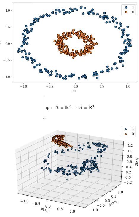
Another way of describing positive definite kernels and RKHS con-sists in defining a feature map φ : X → H where H is a Hilbert space. Then any function in Hkcan be written f(x) = ⟨φ(x), θ⟩HIn a nutshell the function φ is called feature map because it “extracts characteristic elements from a vector”. Usually a feature map takes a vector in an input space with low dimension and maps it to a potentially infinite dimensional Hilbert space. Put it differently, any function in Hk is the composition of linear functional θ∗with a non linear feature map φ. Thus if the feature map φ is fixed (which is equivalent to fixing the kernel), it is possible to “learn” with a linear class of functions θ∈ H (seeFigure 2.3). If we note
ϕ=(φ(x1) . . . φ(xN))
the “matrix” where each column represents the feature map evalu-ated at the point xiwith 1 ⩽ i ⩽ N, the regularized risk minimization with the least square loss reads
Rλ(θ, s) = 1 2N ϕTθ −(y i)Ni=1 22+ λ 2 ∥θ∥ 2 2.
and if λ > 0 the unique minimizer is θs = ( ϕϕT/N+ λI H )−1ϕ. This is an Ot ( dim(H)2(N + dim H)).
time complexity algorithm. This algorithm seems more appealing than its kernel counterpart when many data are given since once the space H has been fixed, the algorithm is linear in the number of training points. However many questions remains. First although it is possible to design a feature map ex nihilo, can we design systemat-ically a feature map from a kernel? For some kernels (e. g. the Gaus-sian kernel) it is well known that the Hilbert space corresponding to it has dimension dim(H) = ∞. Is it possible to find an approximation of the kernel such that dim(H) < ∞? If such a construction is possible and we know that N training data are available, is it possible to have a sufficiently good approximation4with dim(H) ≪ N?
2.1.2 Towards large scale learning with kernels
Motivated by large scale applications, different methodologies have been proposed to approximate kernels and feature maps. This subsec-tion briefly reminds the main approaches based on Random Fourier Features and Nyström techniques. Notice that another line of research concerns online learning method such as NORMA developed in [90], later extended to the operator-valued kernel case by Audiffren and
4 When dim(H) ⩾ N then is it is better to use the kernel algorithm than the feature algorithm. This is called the kernel trick.
−1.0 −0.5 0.0 0.5 1.0 x1 −1.0 −0.5 0.0 0.5 1.0 x2 1 0 y φ: X = R2→ H = R3 ϕ(x)1 −1.0 −0.5 0.0 0.5 1.0 ϕ(x)2 −1.0−0.5 0.00.5 1.0 ϕ (x) 3 −0.2 0.0 0.2 0.4 0.6 0.8 1.0 1.2 1 0
Figure 2.3: We map the two circles in R2 to R3. In R3it is now possible to
separate the circles with a linear functional: a plane. We used the feature map φ(x) = 0.82 cos(1.76x1+ 2.24x2+ 2.75) cos(0.40x1+ 1.87x2+ 5.6) cos(0.98x1−0.98x2+ 6.05) .
Here φ : R2 → R3 has been chosen as a realization of an RFF
map (seeEquation 2.5). A “cleaner” feature map adapted to this problem could have been
φ(x) = x1 x2 x21+ x22 .
Kadri [10]. We start with the seminal work of Rahimi and Recht [139] who show that given a continuous shift-invariant kernel (∀x, z, t ∈ X, k(x + t, z + t) = k(x, z)), it is possible to obtain a feature map called RFF that approximate the given kernel.
2.1.2.1 Random Fourier Features map
The Random Fourier Features methodology introduced by Rahimi and Recht [139] provides a way to scale up kernel methods when kernels are Mercer and translation-invariant. We view the input space Xas a group endowed with the addition. Extensions to other group laws such as Li, Ionescu, and Sminchisescu [98] are described in Sub-subsection 4.2.2.2 within the general framework of operator-valued kernels.
Denote k : Rd× Rd → R a positive definite kernel on X = Rd. A kernel k is said to be shift-invariant or translation-invariant for the addition if for for all (x, z, t) ∈(Rd)3 we have k(x + t, z + t) = k(x, z). Then, we define k0: Rd→ R the function such that k(x, z) = k0(x − z). k0 is called the signature of kernel k. Bochner’s theorem [65] is the theoretical result that leads to the Random Fourier Features.
Theorem 2.3 (Bochner’s theorem). Any continuous positive definite function is the Fourier Transform of a bounded non-negative Borel measure. It implies that any positive definite, continuous and shift-invariant kernel k, has a continuous and positive semi-definite signature k0, which is the Fourier Transform F of a non-negative measure µ. Hence we have k(x, z) = k0(x − z) =∫Rdexp (−i⟨ω, x − z⟩) dµ(ω) = F [k0](ω).
Moreover µ = F−1[k
0]. Without loss of generality, we assume that µ is a probability measure, i. e.∫Rddµ(ω) = 1 by renormalizing the kernel
since ∫ Rd dµ(ω) = ∫ Rdexp (−i⟨ω, 0⟩) dµ(ω) = k0 (0).
and we can write the above equation as an expectation over µ. For all x, z ∈ Rd
k0(x − z) = Eµ [
exp(−i⟨ω, x − z⟩)].
Eventually, if k is real valued we only write the real part, k(x, z) = Eµ[cos⟨ω, x − z⟩]
= Eµ[cos⟨ω, z⟩ cos⟨ω, x⟩ + sin⟨ω, z⟩ sin⟨ω, x⟩]. Let⊕D
j=1xjdenote the Dd-length column vector obtained by stacking vectors xj∈ Rd. The feature map eφ: Rd → R2Ddefined as
(2.4) e φ(x) = √1 D D ⊕ j=1 ( cos ⟨x, ωj⟩ sin ⟨x, ωj⟩ ) , ωj ∼ F−1[k0]i. i. d.
is called a Random Fourier Features (map). Each ωj, j = 1, . . . , D is in-dependently and identically sampled from the inverse Fourier trans-form µ of k0. This Random Fourier Features map provides the fol-lowing Monte-Carlo estimator of the kernel: ek(x, z) = eφ(x)∗φ(z). Us-e ing trigonometric identities, Rahimi and Recht [139] showed that the same feature map can also be written
(2.5) ˜φ(x) = √ 2 D D ⊕ j=1 ( cos(⟨x, ωj⟩ + bj) ) ,
where ωj ∼ F−1[k0], bj ∼ U(0, 2π) i. i. d.. The feature map defined byEquation 2.4andEquation 2.5have been compared in Sutherland and Schneider [167] where they give the condition under wich Equa-tion 2.4 has lower variance than Equation 2.5. For instance for the Gaussian kernel,Equation 2.4has always lower variance. In practice,
Equation 2.5 is easier to program. In this manuscript we focus on random Fourier feature of the form given inEquation 2.4.
The dimension D governs the precision of this approximation, whose uniform convergence towards the target kernel (as defined in Theorem 2.3) can be found in Rahimi and Recht [139] and in more recent papers with some refinements proposed in Sutherland and Schneider [167] and Sriperumbudur and Szabo [164]. Finally, it is important to notice that Random Fourier Features approach only requires two steps before the application of a learning algorithm: (1) define the inverse Fourier transform of the given shift-invariant ker-nel, (2) compute the randomized feature map using the spectral dis-tribution µ. Rahimi and Recht [139] show that for the Gaussian kernel k0(x − z) = exp(−γ∥x − z∥22), the spectral distribution µ is a Gaussian distribution. For the Laplacian kernel k0(x − z) = exp(−γ∥x − z∥1), the spectral distribution is a Cauchy distribution.
We now focus on another famous way of obtaining feature maps for any scalar valued kernel called the Nyström method.
2.1.2.2 Nyström approximation
To overcome the bottleneck of Gram matrix computations in kernel methods, Williams and Seeger [185] have proposed to generate a low-rank matrix approximation of the Gram matrix using a subset of its columns. Since this feature map is based on a decomposition of the Gram matrix, the feature map resulting from the Nyström method is data dependent. Let k : X2 → R be any scalar-valued kernel and let
s= (xi)Ni=1
be the training data. We note a subsample of the training data sM= (xi)Mi=1
where M ⩽ N and sMis a subsequence of s. Then construct the Gram matrix KMon the subsequence sM. Namely
KM= ( k(xi, xj) ) M i,j=1.
Then perform the singular-valued decomposition KM = UΛUT. The Nyström feature map is given by
˜φ(x) = Λ−1/2UT(⊕M
i=1k(x, xi) )
.
Here M plays the same role as D in the RFF case: it controls the quality of the approximation. Let K be the full Gram matrix on the training data s, let
Kb= (
k(xi, xj)
)i=N,j=M i=1,j=1 .
Then it is easy to verify that ϕTϕ = K
bK†MKTb ≈ K, where K†M is the pseudo-inverse of KM and the quantity KbK†MKTb is a low rank approximation of the Gram matrix K.
2.1.2.3 Random features vs Nyström method
The main conceptual difference between the Nyström features and the Random Fourier Feature is that the Nyström construction is data dependent, while the RFF is not. The advantage of random Fourier feature lies in their fast construction. For N data in Rd, it costs O(NDd) to featurize all the data. For the Nyström features it costs O(M2(M + d)). Moreover if one desires to add a new feature, the RFF methodology is as simple as drawing a new random vector ω ∼ F−1[k0], compute cos(⟨ω, x⟩ + b), where b ∼ U(0, 2π) and concate-nate it the existing feature. For the Nyström features one needs to recompute the singular value decomposition of the new augmented Gram matrix KM+1.
To analyse the RFF and Nyström features authors usually study the approximation error of the approximate Gram ma-trix and the targer kernel ϕTϕ −K (see [55, 142, 190]) or the supremum of the error between the approximated kernel and the true kernel over a compact subset X of the support if k: sup(x,z)∈C⊆X2
˜φ(x)T˜φ(z) − k(x, z) (see Bach [12], Rahimi and Recht [139], Rudi, Camoriano, and Rosasco [144], and Sutherland and Schneider [167]). Because Bartlett and Mendelson [17] showed that for generalization error to be below ϵ ∈ R>0 for kernel methods is O(N−1/2), the number of samples M or D required to reach some ap-proximation error below ϵ should not grow faster than O(M−1/2) for the Nyström method or O(D−1/2) for the RFF method to match kernel learning. Concerning the Nyström method, Yang et al. [190] suggest
that the number of samples M is reduced to O(M−1) to reach an error below ϵ when the gap between the eigenvalues of K is large enough. As a result in this specific case, one should sample M = O(√N) Nyström features to ensure good generalization. On the other hand Rahimi and Recht [140] reported that the generalization performance of RFF learning is O(N−1/2+ D−1/2), which indicates that D = O(N) features should be sampled to generalize well. As a result the com-plexity of learning with the RFF seems not to decrease. However the bounds of Rahimi and Recht [140] are suboptimal and very recently (end of 2016) Rudi, Camoriano, and Rosasco [144] proved that in the case of ridge regression (Equation 2.3), the generalization error is O(N−1/2+ D−1) meaning that D = O(√N) random features are required for good generalization with RFFs. We refer the interested reader to Yang et al. [190] for an empirical comparison between the Nyström method and the RFF method.
2.1.2.4 Extensions of the RFF method
The seminal idea of Rahimi and Recht [139] has opened a large lit-erature on random features. Nowadays, many classes of kernels other than translation invariant are now proved to have an efficient random feature representation. Kar and Karnick [87] proposed random fea-ture maps for dot product kernels (rotation invariant) and Hamid et al. [77] improved the rate of convergence of the approximation error for such kernels by noticing that feature maps for dot product kernels are usually low rank and may not utilize the capacity of the projected feature space efficiently. Pham and Pagh [135] proposed fast random feature maps for polynomial kernels.
Li, Ionescu, and Sminchisescu [98] generalized the original RFF of Rahimi and Recht [139]. Instead of computing feature maps for shift-invariant kernels on the additive group (Rd,+), they used the generalized Fourier transform on any locally compact abelian group to derive random features on the multiplicative group (Rd
>0,∗). In the same spirit Yang et al. [189] noticed that an theorem equivalent to Bochner’s theorem exists on the semi-group (Rd
+,+). From this they derived “Random Laplace” features and used them to approximate kernels adapted to learn on histograms.
To speed-up the convergence rate of the random features approx-imation, Yang et al. [188] proposed to sample the random variable from a quasi Monte-Carlo sequence instead of i. i. d. random vari-ables. Le, Sarlós, and Smola [94] proposed the “Fastfood” algorithm to reduce the complexity of computing a RFF –using structured matrices and a fast Walsh-Hadarmard transform– from Ot(Dd) to Ot(D log(d)). More recently Felix et al. [61] proposed also an algo-rithm “SORF” to compute Gaussian RFF in Ot(D log(d)) but with
bet-ter convergence rates than “Fastfood” [94]. Mukuta and Harada [124] proposed a data dependent feature map (comparable to the Nystro ¨m method) by estimating the distribution of the input data, and then finding the eigenfunction decomposition of Mercer’s integral opera-tor associated to the kernel.
In the context of large scale learning and deep learning, Lu et al. [108] showed that RFFs can achieve performances comparable to deep-learning methods by combining multiple kernel learning and composition of kernels along with a scalable parallel implementation. Dai et al. [51] and Xie, Liang, and Song [186] combined RFFs and stochastic gradient descent to define an online learning algorithm called “Doubly stochastic gradient descent” adapted to large scale learning. Yang et al. [192] proposed and studied the idea of replac-ing the last fully interconnected layer of a deep convolutional neural network [95] by the “Fastfood” implementation of RFFs.
Eventually Yang et al. [191] introduced the algorithm “À la Carte”, based on “Fastfood” which is able to learn the spectral distribution corresponding to a kernel rather than defining it from the kernel. Very recently Kawaguchi, Xie, and Song [88] proposed to use semi-random features which are a tradeoff between the random features based on kernel methods (e. g. RFFs) and the trainable layer in deep learning.
3
B A C K G R O U N DIn this chapter we introduce briefly the mathematical tools used throughout this manuscript. We give a full table of notations, and present elements of functional analysis [93] and abstract hamonic analysis [65]. Then we turn our attention to the case when the func-tions we want to learn are not real-valued, but vector-valued. To learn vector-valued functions we define Operator-Valued Kernels that gen-eralize the scalar-valued kernel presented inChapter 2. We conclude by giving a non-exhaustive list of Operator-Valued Kernels and in which context they have been used.
Contents
3.1 Notations . . . 22 3.1.1 Algebraic structures . . . 22
3.1.2 Topology and continuity . . . 22
3.1.3 Measure theory . . . 23
3.1.4 Vector spaces, linear operators and matrices 24
3.2 Elements of abstract harmonic analysis . . . 26
3.2.1 Locally compact Abelian groups . . . 26
3.2.2 The Haar measure . . . 29
3.2.3 Even and odd functions . . . 30
3.2.4 Characters . . . 30
3.2.5 The Fourier Transform . . . 33
3.2.6 Representations of Groups . . . 35
3.3 On Operator-Valued Kernels . . . 36 3.3.1 Definitions and properties . . . 36
3.3.2 Shift-Invariant OVK on LCA groups . . . . 43
3.3.3 Examples of Operator-Valued Kernels . . . 44
3.3.4 Some use of Operator-valued kernels . . . 48
3.1 notations
In this section we summarize briefly important notions used through-out this document. It is mainly based on books and lecture notes of Cotaescu [49] and Kurdila and Zabarankin [93].
3.1.1 Algebraic structures
We note K any Abelian1 field and call its elements scalars. R is the
1
Commutative.
Abelian field of real numbers and C is the Abelian field of complex numbers. The unit pure imaginary number√−1 ∈ C is denoted i and the Euler constant exp(1) ∈ R is denoted e. N represents the set of natural numbers and Nn, n ∈ N the set of natural numbers smaller or equal to n. For any space S, Sd, d ∈ N represents the Cartesian product space Sd= S × · · · × S. For any two algebraic structures S and S′ we write S ∼= S′ if there exist an isomorphism between these two structures. If a + ib = x ∈ C then x = a − ib ∈ C denotes the complex conjugate. By extension if x ∈ R, x = x ∈ R.
3.1.2 Topology and continuity
In order to define a proper notion of continuity, we focus on topo-logical spaces. A topotopo-logical space is a pair of sets (X, Tx) where X describes the points considered, and Txdescribes the possible neigh-bourhoods. The standard axioms of topology suppose that Tx ⊆ P(X) is a collection of subsets of X such that the empty set and X itself belongs to Tx, any (finite or infinite) union of members of Tx still belongs to Tx and the intersection of any finite number of members of Tx still belongs to Tx. The elements of Tx are called open sets and the collection Tx is a topology on X. If (X, Tx) and (Y, Ty) are topo-logical spaces, a function f is said to be continuous if for every open set V ∈ Ty, the inverse image f−1(V) = { x ∈ X | f(x) ∈ V } is an open subset of Tx. Since the notion of continuity depends on open sets, it depends on the topology of the spaces X and Y.
If (X, Tx) is a topological space and x is a point in X, a neighbour-hood of x is a subset V of X that includes an open set U containing x. A topological space X is said to be Hausdorff (T2) when all distinct points in X are pairwise neighbourhood-separable. i. e. if there exists a neighbourhood U of x and a neighbourhood V of y such that U and V are disjoint. It implies the uniqueness of limits of sequences and existence of nets used throughout this thesis. Therefore in the whole document we always assume that a topological space X is Haussdorff.
A topological space is said to be second countable if it has a count-able base. Every second-countcount-able space is separcount-able and Lindelöf2
(The reverse implications do not hold). A space is metrisable if and 2
Every open cover has a countable subcover.
only if it is second countable.
A topological space is said to be separable if there exists a sequence (xn)n∈N∗ of elements of X such that every nonempty open subsets of
the space contains at least one element of the sequence. Separability plays an important role in numerical analysis because many theorems have only constructive proofs for separable spaces. Such constructive proofs can be turned into algorithms which is the primary goal of this work. In this document we also assume that any topological space is separable if there is no specific mention of the contrary. Moreover we recall that a Hilbert space is separable if and only if it has a countable orthonormal basis (Hence separable Hilbert spaces are second count-able). Hence an operator between two separable Hilbert spaces can be written as an infinite dimensional matrix. In some cases we also introduce Polish spaces which are separable topological spaces X that have at least one metric d such that (X, d) is complete. Then d induces the topology Txof X. As metrisable spaces, Polish spaces are always second countable. Moreover every second countable locally compact Hausdorff space is a Polish space and every separable Banach space is a Polish space.
If X and Y are two topological spaces, we denote by F(X; Y) the topological vector space of functions f : X → Y and C(X; Y) ⊂ F(X; Y) the subspace of continuous functions, endowed with the product topology (topology of pointwise convergence).
3.1.3 Measure theory
A σ-algebra on X is a set M ⊆ P(X) of subsets of X, containing the empty set, which is closed under taking complements and countable unions. A pair (X, M) where X is a set and M is a σ-algebra is called a measure space. The Borel σ-algebra B(X) is a σ-algebra generated by the open sets of X. A measure on a measurable space (X, B(X)) is a map µ : B(X) → R+ which is zero on the empty set and countably additive, i. e. for any subset (Zn)n∈Nis a sequence of pairwise disjoint measurable sets, µ ( ∪ n∈N Zn ) = ∑ n∈N µ(Zn).
We note N(m, σ) the Gaussian distribution with mean m ∈ R and variance σ2 ∈ R. U(a, b) is the uniform distribution with support (a, b) and S(m, σ) is the hyperbolic secant distribution with mean m and variance σ2.
3.1.4 Vector spaces, linear operators and matrices
Given any vector space H over an Abelian field K, the (continuous) dual space1H∗is defined as the set of all continuous linear functionals x∗ : H → K. When H is a vector space, there is a natural duality pairing between H∗ and H defined for all x∗ ∈ H∗ and all z ∈ H as (x∗, z)
H∗,H = x∗(z) = x∗z. The duality paring (·, ·)H∗,H is then a
bilinear form.
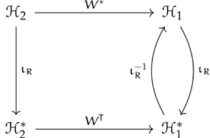
Let H1 and H2 be two vector spaces. We call operator any lin-ear function from H1 to H2. The transpose (or dual) of an oper-ator W : H1 → H2 is defined as WT : H∗
2 → H∗1 such that WT : x∗ 7→ x∗(W). It is characterized by the relation (x∗, Wz)
H∗ 2,H2 = ( WTx∗, z)H∗ 1,H1 for all x ∗ ∈ H∗
2 and all z ∈ H1. An operator is called self-dual when WT= W.
Let H1 and H∈ be two vector space. We set L(H1; H2) to be the space of bounded (linear) operators from H1 to H2. The vector space H1 is called the domain, noted Dom and H2 the codomain. We use the shortcut notation L(H) = L(H; H). Interestingly if H1 and H2 are normed vector spaces, they can be viewed as topological vector spaces, and the notion of continuity coincides with that of bounded-ness. We recall that the norm of a linear operator is given by
∥W∥H∞,H2 = sup x̸=0 ∥Wx∥H2 ∥x∥H1 . If W ∈ L(H1, H2) Ker W = { x ∈ Dom (W) | Wx = 0 }
denotes the kernel (nullspace), which is a vector subspace of the do-main and
Im W = { y ∈ H2| y= Wx, x ∈ Dom (W) }
the image (range) which is a vector subspace of the codomain H2. If H is an Hilbert space on a field K we denote its scalar product by ⟨·, ·⟩Hand its norm by ∥·∥H. When the base field of H is R, ⟨·, ·⟩H is a bilinear form. When the base field of H is C, ⟨·, ·⟩His a sesquilinear form.
1 The continuous dual space is also called topological dual space. This must be differ-entiate from the algebraic dual space, which is the space of linear functionals from the original vector-space to its base field. Hence the continuous dual space is a subset of the algebraic dual space. The continuous and the algebraic dual space only match when considering finite dimensional vector-spaces
Let H be a Hilbert space. From Riesz’s representation theorem, there is a unique isometric isomorphism ιR : H → H∗ such that for any x and y ∈ H, (ιR(x), y)H∗,H = ⟨x, y⟩H and ∥ιR(x)∥H∗ = ∥x∥H. The
Riesz map ιR is self-dual, thus if H is a Hilbert space, H is reflexive. i. e. H∗∗ ∼= H. When the base field of H is C, then the Riesz map ιR is an anti-linear form since ⟨·, ·⟩His sesquilinear and (·, ·)H∗,His bilinear. In the same way when the base field of H is R then ιR is linear since both ⟨·, ·⟩Hand (·, ·)H∗,Hare bilinear. If H is a Hilbert space we make the dual space H∗ a Hilbert space by endowing it with the inner product ⟨x∗, z∗⟩
H∗ = ⟨ι−1R (x∗), ι−1R (z∗)⟩H for all x∗, z∗∈ H∗.
Let H1 and H2 be two Hilbert spaces. The adjoint of an operator W : H1 → H2 is the unique mapping W∗ : H2 → H1 such that ⟨W∗x, z⟩
H1 = ⟨x, Wz⟩H2 for all x ∈ Dom (W∗), z ∈ Dom (W). Its ex-istence is guaranteed by Riesz’s representation theorem. An operator W : Dom (W) ⊆ H → H is said to be symmetric when W∗ = W, and self-adjoint when W is bounded, symmetric, Dom (W∗) = Dom (W) and Dom (W) is dense in H. If W is bounded, symmetric and Dom (W) = H then W is self-adjoint. Notice that the transpose is linked to the adjoint by the relation W∗ = ι−1
R WTιR. When H is a Hilbert space, if x ∈ H, we always define x∗ ∈ H∗to be
x∗= ιR(x) = ⟨x, ·⟩H. H2 H1 H2∗ H∗1 W∗ ιR ιR WT ι−R1
Figure 3.1: Riesz map, dual spaces and adjoints.
Let H be a separable Hilbert space and let (ei)i∈N∗ be a basis of
H. We call (e∗
i)i∈N∗ the dual basis of H, the basis of H∗ such that
for all i, j ∈ N∗, e∗
i(ej) = ⟨ei, ej⟩H = δij. In the whole document we consider that H∗ is always equipped with the dual basis of H. For a vector x ∈ H with a basis (ei)i∈N∗ we write xi = e∗i(x). For a linear operator W : H1 → H2 where H1 and H2 are Hilbert spaces with respective basis (ei)i∈N∗ and (ej′)j∈N∗, we note Wi = Wei and
Wij= e∗j(Wei). Eventually given two separable Hilbert spaces H1and H2, an operator W : H1 → H2, (ei)i∈N∗ a basis of H1 and (ei′)i∈N∗ a
basis of H2we have (WT)
We call matrix M of size (m, n) ∈ N2on an Abelian field K a collec-tion of elements M = (mij)1⩽i⩽m,1⩽j⩽n, mij ∈ K. We note Mm,n(K) the vector space of all matrices. If H1 and H2 are two separable Hil-bert spaces on an Abelian field K, any linear operator L ∈ L(H1; H2) can be viewed as a (potentially infinite) matrix. Let n = dim(H1), m = dim(H2) and let B = (ei)ni=1 and C = (ei′)mi=1 be the respec-tive bases of H1 and H2. We note matB,C : L(H1; H2) → Mm,n(K) such that M = matB,C(L) = (e′∗jLei)1⩽i⩽n,1⩽j⩽m ∈ Mm,n(K). Let M1∈ Mm,n(K) and M2 ∈ Mn,l(K). The product between two matri-ces is written M1M2 ∈ Mm,l(K) and obey (M1M2)ij=∑nk=1MikMkj. Given two linear operator L1 ∈ L(H1; H2) and L2 ∈ L(H2; H3) we have L1L2∈ L(H1; H3) and i
matB,D(L1L2) = matB,C(L1)matC,D(L2).
The operator matB,C is a vector space isomorphism allowing us to identify L(H1; H2) with Mmn(K) where n = dim(H1) and m = dim(H2). All these notations are summarized in Tables 3.1 and 3.3.
3.2 elements of abstract harmonic analysis 3.2.1 Locally compact Abelian groups
Definition 3.1 (Locally Compact Abelian (LCA) group.). A group X endowed with a binary operation ⋆ is said to be a Locally Compact Abelian group if X is a topological commutative group w. r. t. ⋆ for which every point has a compact neighborhood and is Hausdorff (T2).
Moreover given a element z of a LCA group X, we define the set z ⋆ X = X ⋆ z = { z ⋆ x |∀x ∈ X } and the set X−1={x−1 ∀x ∈ X}. We also note e the neutral element of X such that x ⋆ e = e ⋆ x = e for all x∈ X. Throughout this thesis we focus on positive-definite functions. Let Y be a complex separable Hilbert space. A function f : X → Y is positive definite if for all N ∈ N and all y ∈ Y,
(3.1) N ∑ i,j=1 ⟨ yi, f ( x−1j ⋆ xi ) yj ⟩ Y⩾0 for all sequences (yi)i∈N∗
N ∈ Y
N and all sequences (x i)i∈N∗
N ∈ X
N. If Yis real we add the assumption that f(x−1) = f(x)∗ for all x ∈ X. A consequence is that a positive-definite function is bounded, as shown by Falb [60], ∥f(x)∥Y,Y ⩽ 2∥f(e)∥Y,Y for all x ∈ X, however positive-definite functions are not necessarily continuous. This motivates the introduction of functions of positive type which are nothing but con-tinuous positive-definite function.
Table 3.1: Mathematical symbols and their signification (part 1).
Symbol Meaning
:= Equal by definition.
N The semi-group of natural numbers.
K Any non-discrete Abelian field endowed with an abso-lute value. Elements of K are called scalars.
R The Abelian field of real numbers. C The Abelian field of complex numbers.
U The circle group of complex numbers with unit mod-ule.
i ∈ C Unit pure imaginary number i2 := −1. e ∈ R Euler constant.
e∈ X The neutral element of the group X.
δij Kronecker delta function. δij= 0 if i ̸= j, 1 otherwise. ⟨·, ·⟩2 Euclidean inner product.
∥·∥2 Euclidean norm. X Input space. b
X The Pontryagin dual of X when X is a LCA group. Y Output space (Hilbert space).
H Feature space (Hilbert space).
⟨·, ·⟩Y The canonical inner product of the Hilbert space Y. ∥·∥Y The canonical norm induced by the inner product of
the Hilbert space Y.
F(X; Y) Topological vector space of functions from X to Y. C(X; Y) The topological vector subspace of F of continuous
functions from X to Y.
L(H; Y) The set of bounded linear operator from a Hilbert space H to a Hilbert space Y.
∥·∥Y,Y′ The operator norm ∥Γ∥Y,Y′ = sup∥y∥
Y=1∥Γy∥Y′ for all
Γ ∈ L(Y, Y′)
Mm,n(K) The set of matrices of size (m, n).
L(Y) The set of bounded linear operator from a Hilbert space Y to itself.
L+(Y) The set of non-negative bounded linear operator from a Hilbert space H to itself.
B(X) Borel σ-algebra on a topological space X. µ(X) A scalar positive measure of X.
Leb(X) The Lebesgue measure of X. Haar(X) A Haar measure of X.
Table 3.3: Mathematical symbols and their signification (part 2).
Symbol Meaning
Prµ,ρ(X) A probability measure of X whose Radon-Nikodym derivative (density) with respect to the measure µ is ρ.
F[·] The Fourier Transform operator.
F−1[·] The Inverse Fourier Transform operator. ess sup The essential supremum.
Lp(X, µ) The Banach space of |·|p-integrable function from (X, B(X), µ) to C for p ∈ R+.
Lp(X, µ; Y) The Banach space of ∥·∥pY (Bochner)-integrable func-tion from (X, B(X), µ) to Y for p ∈ R+. Lp(X, µ, R) := Lp(X, µ).
⊕D
j=1xi The direct sum of D ∈ N vectors xi’s in the Hil-bert spaces Hi. By definition ⟨⊕Dj=1xj,⊕Dj=1zj⟩ = ∑D j=1⟨xj, zj⟩Hi [11]. ∥·∥p The Lp(X, µ, Y) norm. ∥f∥ p p := ∫ X∥f(x)∥ p Ydµ(x). When X = N∗, Y ⊆ R and µ is the counting measure and p = 2 it coincide with the Euclidean norm ∥·∥2 for finite dimensional vectors.
∥·∥∞ The uniform norm ∥f∥∞ = ess sup { ∥f(x)∥Y| x∈ X } = limp→∞∥f∥p.
T The transpose operator of a linear operator. ∗ The adjoint operator of a linear operator.
|Γ | The absolute value of the linear operator Γ ∈ L(Y), i. e. |Γ |2 = Γ∗Γ.
Tr [Γ] The trace of a linear operator Γ ∈ L(Y).
σ(Γ) The spectrum of the bounded linear operator Gamma∈ L(Y) where Y is a Hilbert space, i. e. σ(Γ) = { λ∈ C | ∄s, s(λe − Γ) = e }.
λi(Γ) The i-th eigenvalue of Γ ∈ L(Y), ranked by increasing modulus, where Y is a separable Hilbert space and i ∈ N∗.
ρ(Γ) The spectral radius of the linear operator Γ i. e. ρ(Γ) = sup { |λ| | λ ∈ σ(Γ) }.
∥·∥σ,p The Schatten p-norm, ∥Γ∥ p
σ,p = Tr [|Γ|
p]for Γ ∈ L(Y), where Y is a Hilbert space. Note that ∥Γ∥σ,∞= ρ(Γ) ⩽ ∥Γ∥Y,Y.
≽ “Greater than” in the Loewner partial order of opera-tors. Γ1≽Γ2if σ(Γ1− Γ2) ⊆ R+.
R The one point compacification of the real line R ∪ {∞ }.
∼
= Given two sets X and Y, X ∼= Y if there exists an iso-morphism φ : X → Y.