HAL Id: hal-00543316
https://hal.archives-ouvertes.fr/hal-00543316
Submitted on 6 Dec 2010
HAL is a multi-disciplinary open access
archive for the deposit and dissemination of
sci-entific research documents, whether they are
pub-L’archive ouverte pluridisciplinaire HAL, est
destinée au dépôt et à la diffusion de documents
scientifiques de niveau recherche, publiés ou non,
Anisotropic and hyperelastic identification of in vitro
human arteries from full-field optical measurements
Stéphane Avril, Pierre Badel, Ambroise Duprey
To cite this version:
Stéphane Avril, Pierre Badel, Ambroise Duprey. Anisotropic and hyperelastic identification of in vitro
human arteries from full-field optical measurements. Journal of Biomechanics, Elsevier, 2010, 43 (15),
pp.2978-2985. �10.1016/j.jbiomech.2010.07.004�. �hal-00543316�
Anisotropic and hyperelastic identification
1
of in vitro human arteries from full-field
2
optical measurements
3
St´ephane Avril, Pierre Badel, Ambroise Duprey
4
Center for Health Engineering
5
Ecole Nationale Sup´erieure des Mines de Saint-´
Etienne
6
PECM - CNRS UMR 5146 ; IFRESIS - INSERM IFR 143
7
158 Cours Fauriel, 42023 SAINT-´
ETIENNE cedex 2, FRANCE
8
Abstract
9
In this paper, we present a new approach for the bi-axial characterization of in vitro human arteries
10
and we prove its feasibility on an example. The specificity of the approach is that it can handle
het-11
erogeneous strain and stress distributions in arterial segments. From the full-field experimental data
12
obtained in inflation/extension tests, an inverse approach, called the virtual fields method (VFM),
13
is used for deriving the material parameters of the tested arterial segment. The obtained results are
14
promising and the approach can effectively provide relevant values for the anisotropic hyperelastic
15
properties of the tested sample.
16
1
Introduction
17
It is well assessed that, despite biochemical and hemodynamical factors play a primary role in the
develop-18
ment of most vascular disorders, solid mechanics models may contribute to understand their genesis and
19
progression. The realism of models in solid mechanics depends significantly on the mechanical properties
20
used as input parameters. Therefore, characterizing the biomechanical properties of arteries remains an
21
essential issue.
22
In vivo measurements with ultrasounds or magnetic resonance imaging (MRI) techniques provide
23
relevant information on the vascular behavior [Slager et al., 2000, Masson et al., 2008, Avril et al., 2009]
24
although they are not sufficient for a rigorous determination of arterial wall constitutive equations. To
25
investigate the passive structural response of the arterial tissue, a large variety of in vitro experimental
26
protocols are available [Humphrey, 2002].
27
Among them, inflation/extension of arterial segments are physiologically meaningful tests since the
28
in vivo loading conditions may be reproduced and the native geometry is preserved [Hayashi, 1993].
29
Classically, for the analysis, it is assumed that the artery is a perfect cylinder and that the loading
30
induces a homogeneous stress and strain distribution [Humphrey, 2002, Fung, 1993]. These assumptions
31
provide a framework for deriving stress-strain curves and to fit them by appropriate constitutive models.
However, inverse approaches should generally be employed since stresses and strains are always
het-33
erogeneous, because of noncylindrical shape [Holzapfel, 2004, Humphrey, 1999], locally varying material
34
properties or experimental artifacts like edge effects [Arimitsu et al., 1995].
35
The combination of 3-D deformation measurements [Rastogi, 1999, Foster, 1978, Viotti et al., 2008,
36
Matthys et al., 1991, Genovese, 2007, Genovese, 2009, Sutton et al., 2007] and inverse approaches [Avril
37
et al., 2008] is now very common in solid mechanics but it is still under-employed for identifying the
38
anisotropic hyperelastic properties of the arterial tissues [Seshaiyer and Humphrey, 2003, Einstein et al.,
39
2005]. Moreover, the Virtual Fields Method [Gr´ediac et al., 2006], which is an inverse method specifically
40
dedicated to full-field data, has never been used for the mechanical identification of arterial tissues
41
although it has very relevant assets: insensitivity to the uncertainty of boundary conditions [Gr´ediac
42
et al., 2006], robustness [Avril et al., 2004], fast convergence [Avril and Pierron, 2007].
43
This paper attempts to give a new contribution for addressing the mechanical identification of arterial
44
tissues by presenting an implementation of the Virtual Fields Method to full-field experimental data
45
measured on the whole surface of an arterial segment during inflation/extension tests. The objective of
46
the paper is to present the principle of the approach and to prove its feasibility on an example.
47
2
Materials and Methods
48
2.1
Materials
49
Results reported in this paper are obtained on a fairly straight segment of a human ascending aorta (initial
50
length: L0' 35 mm, initial average radius: R0' 10 mm, initial average thickness: e0' 1.3 mm). This
51
vascular segment has been obtained from a cadaveric 65 years old female donor. All procedures were
52
carried out in accordance with the guidelines of the Institutional Review Board of the University Hospital
53
Centre of Saint-Etienne, France. After gently cleaning the artery with physiological solution, two side
54
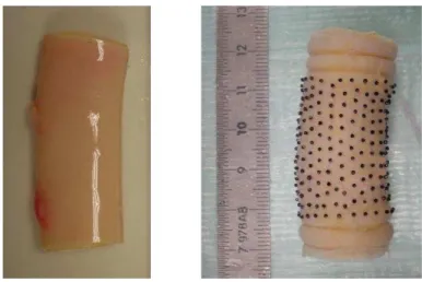
branches were clamped with surgical suture threads (Fig. 1).
55
2.2
Experiments
56
This study results from a collaboration between the University of Basilicata (Italy) and Ecole des Mines
57
de Saint-Etienne (France). The experimental setup was developed at the University of Basilicata and
58
presented in a companion paper [Genovese, 2009]. The current paper focuses on the inverse approach
59
and all the details about the experimental techniques may be found in [Genovese, 2009].
60
The sample was mounted on the in vitro rig and preconditioned via 8 pressurization cycles from p =
0 to p = 80 mmHg (10.5 kPa) and then 8 cycles of axial stretching from L/L0= 1 to L/L0 = 1.4. Then,
62
different sets of inflation/extension tests were performed.
63
Let Ψt denote the geometrical deformation of the artery induced by the loading at time t, such as
64
x(t) = Ψt(x0), where x(t) is the position vector of a material point at t and x0 is the initial position
65
vector of the same material point.
66
The vascular segment is covered with N (N ' 300) black spherical markers (Fig. 1). The markers
67
were fixed with cyanoacrylate adhesive which was shown not to diffuse in the tissues [Holzapfel et al.,
68
2007]. The optical measurement presented in [Genovese, 2009] provides a point-wise evaluation of Ψt at
69
all the points where a marker has been bonded, with an accuracy of 0.17 mm.
70
During all the inflation/extension tests, the artery remains in a bath of physiological solution. The
71
optical technique was calibrated accounting for the bath of physiological solution around the artery
72
[Genovese, 2009]. However the artery was not hydrated while we bonded the markers. This lasted less
73
than one hour. This could be reduced in the future by using glue that activates with water.
74
2.3
Derivation of the field of Green-Lagrange strain tensors
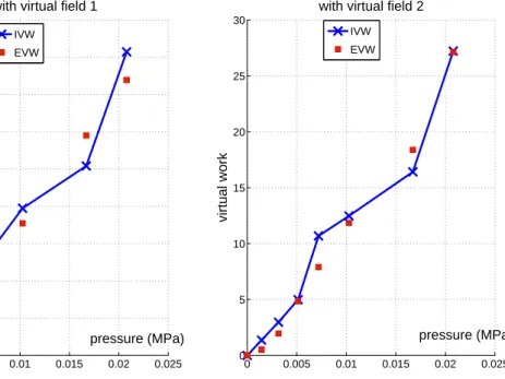
75
The surface of the artery is meshed for interpolating Ψtacross the whole artery from the data measured
76
at the marker position. Triangular elements with linear interpolation functions are used. The mesh is
77
defined using a Delaunay triangularization algorithm applied onto the marker initial positions (actually
78
the marker position means the contact position of the marker onto the surface of the artery). Each
79
triangular element is labeled by an index denoted q. Let xq(t) denote the position vector of the center of
80
gravity of each element at time t
81
Eventually, Ψtis known everywhere across the meshed area of the artery. Let Ω be this domain across
82
which the deformation is measured. Ω is defined in the initial configuration because the deformation is
83
Lagrangian. Let ω(t) be the counterpart of Ω in the deformed configuration at time t.
84
All the derivations presented in this paper are based on the theory of finite deformations [Ogden,
85
1997]. Let F(x0, t) denote the deformation gradient:
86
F(x0, t) ≡ ∇Ψt(x0)
87
where ∇ is the gradient operator.
88
Then we define the right Cauchy-Green tensor:
89
C(x0, t) ≡ FTF
90
where FT is the transpose of F.
Eventually, we define the Green-Lagrange strain tensor:
92
E(x0, t) ≡ [C − I]/2
93
where I is the identity tensor.
94
2.4
Constitutive equations
95
Arteries in vitro are usually considered as anisotropic visco-hyperelastic materials. Here, the
viscoelas-96
tic properties are not considered and only the instantaneous and monotonic response is modeled, after
97
preconditioning. Pseudo-elasticity can therefore be applied [Fung, 1993]. Hyperelastic models are
con-98
sidered.
99
In these models, the Cauchy stress tensor, denoted S, is deduced from the Green-Lagrange strain
100
tensor such as:
101
S = F : dΦ/dE : FT + λI (1)
where Φ is the strain energy function depending only on E and on material parameters. The term λI
102
comes from the incompressibility and λ is assessed by writing the plane stress condition (S33= 0).
103
Different strain energy functions for the anisotropic hyperelastic behavior of arteries may be found
104
in the literature. Some of them are phenomenological [Fung, 1993, Sun and Sacks, 2005] and others are
105
based on the microstructure [Holzapfel et al., 2000]. In this study, we consider 3 different models:
106
1. the Delfino model [Holzapfel et al., 2000]: Φ0 =1
2β
0[exp (α0(I
1− 3)) − 1] (2)
where β0 and α0 are material parameters and I
1= tr(C).
107
2. the 2-D Fung model [Fung, 1993], which may be written as:
108 Φ = 1 2β £ exp¡α11(E11)2+ α22(E22)2+ α12E11E22 ¢ − 1¤=1 2β [exp(Q) − 1] (3)
where β, α11, α22and α12are material parameters and Eij are the components of the E matrix in
109
the material coordinate system (indice 1 refers to the circumferential direction and indice 2 refers
110
to the axial direction in the local coordinate system).
3. the Holzapfel model [Holzapfel et al., 2000]. This model assigns separate strain energy functions to the media layer and the adventitia layer. The simplest form of the strain energy function may be written: Φ00= c 00 2 (I1− 1) + k00 1 2k00 2 £ exp¡k200(I4− 1)2 ¢ − 1¤+ k 00 1 2k00 2 £ exp¡k002(I6− 1)2 ¢ − 1¤ (4) where c00 and k00
1 are stress-like material parameters, k200 is a dimensionless material parameter;I4
112
and I6 are the squares of the stretch component in the two families of symmetric tissue fibers.
113
Hence, this model prescribes a fiber orientation angle φ for each layer, based usually on analysis of
114
microscopy data. The fiber angles for the specimen used in this work were not known, and so the
115
fiber angles are another material parameter to be determined from the experimental data.
116
2.5
Inverse approach
117
The Virtual Fields Method (VFM) is an approach dedicated to the identification of material parameters
118
from full-field measurements [Gr´ediac et al., 2006, Avril et al., 2004, Avril and Pierron, 2007, Promma
119
et al., 2009]. It is based on the weak form of equilibrium equations.
120
Assuming quasi-static conditions and no body forces, the weak form of equilibrium in the deformed
121
configuration may be written such as:
122 − Z ω(t) S : E∗dv + Z ∂ω(t) t.u∗ds = 0 (5)
where ∂ω(t) is the boundary of the volume in the deformed configuration, vector t denotes the tractions
123
applied onto this boundary (pressure forces and axial load), u∗ is a displacement virtual field which acts
124
as a test function in Eq. 5). E∗ is the strain virtual field deduced from the gradient of u∗:
125 E∗=1 2 ³ ∇u∗+ ∇Tu∗ ´ (6) At position x where a marker is located, u∗1and u∗2 take the following values:
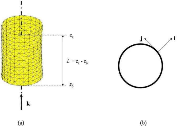
126 u∗1= sin µ πz − zb zt− zb ¶ i u∗2= z − zt zb− zt k (7) where: 127
• vectors i and k are respectively the radial and longitudinal axes in the global cylindrical coordinate
128
system defined in Fig. 2;
129
• z is the component of x along the longitudinal axis: z = x · k ;
130
• zband zt are defined in Fig. 2.
131
The rationale behind this choice of virtual displacements is:
132
• one involves mainly the radial properties (u∗1)
133
• one involves mainly the axial properties (u∗2)
134
• both zero the action of unknown reaction forces or involve their resultant if the resultant is measured
135
[Gr´ediac et al., 2006].
136
Given the previous points, infinity of virtual deformation may be used. The rationale behind the
137
current choice is that the best results are always obtained with the simplest functions. This was proved
138
in different papers [Gr´ediac et al., 2006, Avril et al., 2004, Avril and Pierron, 2007, Promma et al., 2009].
139
This can be interpreted like this: a virtual deformation is a test function. If the test function is very
140
smooth, it will average out the randomly distributed errors contained in the experimental data.
141
Eq. 7 only gives the values of the virtual displacement at marker positions. Between the marker
142
positions, the values of u∗1 and u∗2 are interpolated linearly.
143
Moreover, regarding the external virtual work, it can be written:
144 Z ∂ω(t) t.u∗1ds = Z ∂ω(t) kt.u∗1 p(t)ds Z ∂ω(t) t.u∗2ds = Z ∂ω(t) kt.u∗2 p(t)ds + F(t) (8)
where ktis the unit outer normal vector at t, F(t) is the axial resultant load measured by a load cell.
145
As S is deduced from experimental data, Eq. 5 cannot be satisfied exactly and the principle of the
146
inverse method [Gr´ediac et al., 2006] is to minimize the squares of residuals, as defined in the following
147 cost function: 148 ζ(β, α11, α22, α12) = X k X m " − Z ω(tm) S : E∗kdv + p(tm) Z ∂ω(tm) ktm.u ∗k ds + δ k2F(t) #2 (9)
where m labels the time when a measurement is achieved and k labels the virtual field (k = 1, 2); δk2=0
149
if k = 1 and δk2=1 if k = 2.
150
Considering the interpolation of all quantities with the triangular mesh, the previous integrals in the
151
principle of virtual work may be changed into discrete sums.
152 ζ(β, α11, α22, α12) = X k X m " −X q S(xq,m) : E∗k(xq,m)A(xq,m)e(xq,m) + p(t m) X q kt(xq,m).u∗k(xq,m)A(xq,m) + δk2F(t) #2 (10) where A(xq,m) denotes the area of triangular element q at time t
mand e(xq,m) denotes the thickness of
153
the artery1at xq at time t
m. E∗k is derived from the virtual displacements u∗k using Eq. 6. The virtual
154
displacements u∗k are defined in Eq. 7. The value of p are experimental data and S is derived using
155
Eq. 1. It must be noted that the model parameters are involved in S. All the incremental steps are taken
156
into account as the squares of residuals of each incremental step, denoted m, are summed up.
157
Cost function ζ figures the quadratic gap between the internal virtual work (IVW) and the external virtual work (EVW) where:
IVWk,m= e0 X q S(xq,m) : E∗k(xq,m)A(xq,0) EVWk,m= p(tm) X q kt(xq,m).u∗k(xq,m)A(xq,m) + δk2F(t) (11)
Cost function ζ and IVW are driven by the choice of the unknown material parameters. Eventually,
158
the cost function can be minimized through an iterative scheme using the Nelder-Mead algorithm [Nelder
159
and Mead, 1965]. This yields the unknown material parameters.
160
3
Results
161
A sample was tested for proving the feasibility of the approach (Fig. 1 and Fig. 2). We report data
162
corresponding to 8 pressure levels distributed between 0 and 150 mmHg at L/L0 = 1.1 (Fig. 3 and
163
Fig. 4).
164
The results obtained with the VFM are reported in Tab. 1 for the Fung model. Convergence of the
165
Nelder Mead optimization routine was reached in nearly 10 minutes. The identified values for the Fung
166
material parameters of the artery are consistent with the range orders reported in the literature [Holzapfel
167
1Due to the incompressibility assumption, A(xq,m)e(xq,m) = A(xq,0)e
parameter β α11 α22 α12
identified value 5 kPa 14.5 7 0.1
Table 1: Results obtained with experimental data for the Fung model.
et al., 2000, Fung, 1993]. Parameter β is usually around 10 kPa. It is interesting to notice the large
168
difference between the value of α11 and α22. It means that there is a large anisotropy in this specimen,
169
which has already been reported in the literature [Holzapfel et al., 2000].
170
It can be observed in Fig. 5 that the gap between the external virtual work and the internal virtual
171
work is very low for the obtained material parameters.
172
4
Discussion
173
4.1
Application to the other constitutive models
174
4.1.1 The Delfino model
175
The material parameters of Eq. 2, namely α0 and β0 can be identified using only u∗1. This means that
176
only the circumferential response is used for the identification. The results obtained with the VFM for
177
these two material parameters are: β0 = 1.5 kPa and α0 = 4.6.
178
However, it is interesting to notice in Fig. 6 that the gap between IVW and EVW remains very large
179
for u∗2 when computed with the constitutive equations of Eq. 2 and the material parameters reported
180
above. This indicates irrelevancy of the isotropic assumption. This justifies the choice of anisotropic
181
laws.
182
4.1.2 The Holzapfel model
183
Here, having access only to measurements on the surface of the artery, it is only possible to identify the
184
average strain energy function across the whole thickness, but not separately strain energy functions of the
185
media layer and of the adventitia layer. If, as in [Marra et al., 2006], the strain energy function is assumed
186
homogeneous across the thickness, then a mean fiber angle and mean values of the other parameters of the
187
Holzapfel model can be identified by the VFM. The obtained results are: c00 = 0.4 kPa, k00
1 = 8.7 kPa,
188
k00
2 = 5.4 and φ = 27◦. These results show that parameters of a Holzapfel model may be retrieved by the
189
VFM.
190
Fiber angles and material parameters in human arteries are usually different for the media and the
191
adventitia. Only average values are reported here. A separate identification of media and adventitia
192
constitutive equations would be possible by mechanical separation of the layers of the human artery, as
shown in [Holzapfel et al., 2000].
194
4.1.3 Material heterogeneities
195
Arteries may also have properties varying along the axis. The VFM was already applied successfully to the
196
identification of nonlinear heterogeneous behavior for metals [Sutton et al., 2008]. The implementation
197
of a similar approach for arteries is possible but it will require that the spatial resolution is adapted to
198
the length scale of local variations of the material properties. This may be achieved by employing 3-D
199
digital image correlation, as shown in [Sutton et al., 2007].
200
4.2
Discussions for α
12in the Fung model
201
Parameter α12is the coupling factor between E11and E22in the exponential of the strain energy function.
202
It means that α12 characterizes the effect of the circumferential strain onto the axial response, or
vice-203
versa. A value of 0.1 was found for parameter α12 (Tab. 1). For obtaining this result, the algorithm was
204
initialized according to values2 reported in [Fung, 1993].
205
However, it must be noted that the results regarding α12 are significantly affected by the value input
206
for initializing the optimization algorithm. This may indicate a lack of sensitivity of the cost function to
207
α12, inducing the existence of a valley in the cost function.
208
The dependence of the VFM to the initializing values was not observed for the Holzapfel model.
209
Nevertheless, in the Holzapfel model, the exponential part is driven by only 3 material parameters,
210
whereas the exponential part of the Fung model is driven by 4 material parameters. This supplementary
211
material parameter in the Fung model does not affect sufficiently the value of cost function ζ in Eq. 10,
212
inducing the lack of sensitivity to α12. If one would like to increase the sensitivity to α12, one would
213
have to consider the response of the artery not only to incrementally varying pressures, but also to
214
incrementally varying stretches in the axial direction, and to include these responses in the definition of
215
cost function ζ. This will be considered in future studies.
216
4.3
Implementation of the identified model in a FE code
217
In [Sun and Sacks, 2005], the implementation of the Fung model in a FE code was discussed. In order
218
to check the feasibility of utilizing this model with the parameters that we identified here (Tab. 1),
219
computations were achieved on the geometry of the artery with the Abaqus° software. The geometry ofR
220
the model is a 33.8 mm long cylinder with an initial diameter of 21.5 mm, and initial thickness of 1.3 mm.
221
2Initial values: β=29kPa, α
It was meshed with 1276 membrane elements (M3D4R type in Abaqus°). The Fung model is a built-inR
222
feature of Abaqus°, which requires the definition of a local coordinate system related to the anisotropyR
223
directions and the constitutive parameters reported in Tab. 1. No residual stress was incorporated in this
224
model. One end of the cylinder was clamped. Regarding the other end, radial displacements were fixed
225
and a longitudinal displacement was prescribed, corresponding to L/L0= 1.1. The different experimental
226
pressure steps were applied successively. The resolution of the problem was performed using an implicit
227
scheme accounting for large strains.
228
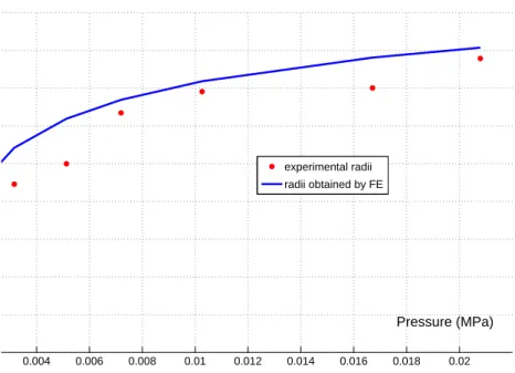
A comparison of the average radii computed by Abaqus° to the measured average radii is shown inR
229
Fig. 7. The comparison is made for the cross section located at z = (zb+ zt)/2, i.e. at midspan. The
230
results show a good agreement.
231
However, the radii computed by FE model are slightly larger than the experimental ones. It may be
232
induced by the fact that, in the model, we neglected the pressure applied by the physiological bath on
233
the external surface of the artery (about 5 mmHg ' 0.7 kPa at the midspan of the arterial segment).
234
Discrepancies may also be induced by a difference between the experimental boundary conditions and
235
the actual ones at the ends. For the FE model, the boundary conditions were of clamping type at both
236
ends, whereas the actual ones are less rigid.
237
It is worth noting here that this discussion about the boundary conditions at both ends does not affect
238
the results obtained by the VFM. Indeed, the effect of unknown reaction forces and parasitic motions at
239
both ends is filtered out by the VFM. This is an essential asset of the VFM, as shown in [Gr´ediac et al.,
240
2006].
241
4.4
Derivation of average stress/strain curves
242
It was shown that the identified Fung model can be used to derive stress/strain curves of the artery, both
243
in the circumferential direction and in the axial direction. Results are presented in the appendices.
244
5
Conclusion
245
In conclusion, results presented in this work are promising regarding the application of the virtual fields
246
method (VFM) for identifying the anisotropic hyperelastic properties of arteries. An innovative
experi-247
mental device has been set up, calibrated and validated for characterizing arterial mechanical properties.
248
It is now important to carry out a large number of experiments for validating the approach with
249
different sets of data and different tests. Other perspectives concern more complex loading conditions
and more sophisticated models. More especially, next steps will consist in (i) considering the possible
251
heterogeneity of the properties and geometry of the artery wall, (ii) processing data from different loading
252
cases (including torsion), (iii) and considering independently the different layers of arteries and the
253
residual stresses. Achievement of these steps will require optimal spatial resolution and accuracy of the
254
measurement technique, employing for instance 3-D digital image correlation [Sutton et al., 2007].
255
6
Acknowledgements
256
The authors would like to thank Professeur Jean-Pierre Favre and to his staff in the department of
257
cardiovascular surgery at the University Hospital of Saint-Etienne (France), for their help in preparing
258
the specimen tested in this study. The authors are also very grateful to Dr. Katia Genovese for the
259
experimental work. This study is part of the Imandef project (Grant ANR-08-JCJC-0071) funded by the
260
ANR (French National Research Agency).
261
7
Appendices
262
7.1
Appendix A
263
In this section, we show that the identified Fung model can be used to derive a stress/strain curve of the
264
artery in the circumferential direction and that this curve is in agreement with the average stress/strain
265
curve deduced from experimental data.
266
The average circumferential Green-Lagrange strain is defined by:
267 ˜ E11(t) = 1 2 õ ¯ R R0 ¶2 − 1 ! (12) where ¯R(t) is the average radius of the best fitting circle at time t at x3= (xb3+ xt3)/2 and R0is ¯R(t) at
268
t = 0.
269
The circumferential stress component, denoted ˜S11, should satisfy the Laplace law everywhere:
270 ˜ S11(t) = p(t) ¯R(t) ¯ e(t) (13)
where ¯e(t) is the average thickness at the midspan of the arterial segment.
271
We compare the value of ˜S11(t) and ¯S11(t), where ¯S11(t) is the value deduced from ˜E11 by applying
272
directly the Fung model of Eq. 3 to ˜E11 with the assumption ˜E22 = 0. The parameters for the Fung’s
273
model are the ones that are reported above in Tab. 1.
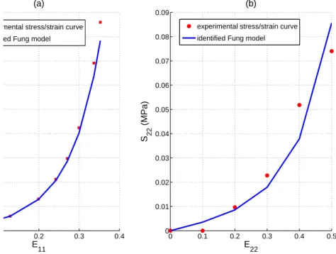
Results shown in Fig. 8a are in agreement. This means that the material parameters identified in
275
the circumferential direction are consistent with a standard procedure (plotting stress/strain curves from
276
pressure/diameter measurements). The advantage of the VFM is that the properties in the axial direction
277
were also identified simultaneously.
278
7.2
Appendix B
279
In this appendix, we show that the identified Fung model can be used to derive a stress/strain curve of
280
the artery subjected to a tensile test in the axial direction and that this curve is in agreement with the
281
average stress/strain curve deduced from experimental data.
282
The axial Green-Lagrange strain is defined by:
283 ˜ E22(t) = 1 2 õ L L0 ¶2 − 1 ! (14) where L(t) is the length of the arterial segment at time t.
284
The axial stress component, denoted ˜S22 should satisfy:
285
˜
S22(t) = F(t)
2π ¯R(t)¯e(t) (15)
We compare the value of ˜S22(t) and ¯S22(t) , where ¯S22(t) is the value deduced from ˜E22 by applying
286
directly the Fung model of Eq. 3 to ˜E22 with the assumption ˜E11 = 0. The parameters for the Fung’s
287
model are reported in Tab. 1.
288
Results shown in Fig. 8b are in agreement. This means that the material parameters identified in the
289
axial direction are in agreement with a classical analysis consisting in plotting stress/strain curves. The
290
advantage of the VFM is that the properties in the axial direction were identified using only one stretch
291
value, whereas a full tensile test was required in the axial direction for plotting the stress/strain curve
292
with the standard analysis.
293
References
294[Arimitsu et al., 1995] Arimitsu, Y., Nishioka, K., , and Senda, T. (1995). A study of Saint-Venant’s
295
principle for composite materials by means of internal stress fields. Journal of Applied Mechanics,
296
62:53–62.
[Avril et al., 2008] Avril, S., Bonnet, M., Bretelle, A.-S., Gr´ediac, M., Hild, F., Ienny, P., Latourte, F.,
298
Lemosse, D., Pagano, S., Pagnacco, E., and Pierron, F. (2008). Identification from measurements of
299
mechanical fields. Experimental Mechanics, 48(5):381–402.
300
[Avril et al., 2004] Avril, S., Gr´ediac, M., and Pierron, F. (2004). Sensitivity of the virtual fields method
301
to noisy data. Computational Mechanics, 34(6):439–452.
302
[Avril et al., 2009] Avril, S., Huntley, J., and Cusack, R. (2009). In-vivo measurements of blood viscosity
303
and wall stiffness in the carotid using PC-MRI. European Journal of Computational Mechanics, 18(1):9–
304
20.
305
[Avril and Pierron, 2007] Avril, S. and Pierron, F. (2007). General framework for the identification of
306
constitutive parameters from full-field measurements in linear elasticity. International Journal of Solids
307
and Structures, 44:4978–5002.
308
[Einstein et al., 2005] Einstein, D., Freed, A., Stander, N., Fata, B., and Vesely, I. (2005). Inverse
309
parameter fitting of biological tissues: A response surface approach. Annals of Biomedical Engineering,
310
33(12):1819–1830.
311
[Foster, 1978] Foster, C. (1978). Measurement of radial deformations in thin-walled cylinders.
Experi-312
mental Mechanics, 18:426–430.
313
[Fung, 1993] Fung, Y. (1993). Biomechanics: Mechanical Properties of Living Tissues. New York:
314
Springer.
315
[Genovese, 2007] Genovese, K. (2007). Radial metrology application to whole-body measurement on
316
hyperelastic tubular samples. Optics and Lasers in Engineering, 45(11):1059–1066.
317
[Genovese, 2009] Genovese, K. (2009). A video-optical system for time-resolved whole-body measurement
318
on vascular segments. Optics and Lasers in Engineering, 47:995–1008.
319
[Gr´ediac et al., 2006] Gr´ediac, M., Pierron, F., Avril, S., and Toussaint, E. (2006). The virtual fields
320
method for extracting constitutive parameters from full-field measurements: a review. Strain, 42:233–
321
253.
322
[Hayashi, 1993] Hayashi, K. (1993). Experimental approaches on measuring the mechanical properties
323
and constitutive laws of arterial walls. ASME Journal of Biomechical Engineering, 115:481–488.
[Holzapfel, 2004] Holzapfel, G. (2004). Experimental approaches on measuring the mechanical properties
325
and constitutive laws of arterial walls. Encyclopedia of computational mechanics. Solids and structures,
326
2:605–635.
327
[Holzapfel et al., 2000] Holzapfel, G., Gasser, T., and Ogden, R. (2000). A new constitutive framework
328
for arterial wall mechanics and comparative study of material models. Journal of Elasticity, 61:1–48.
329
[Holzapfel et al., 2007] Holzapfel, G., Sommer, G., Auer, M., Regitnig, P., and Ogden, R. (2007).
Layer-330
specific 3d residual deformations of human aortas with non-atherosclerotic intimal thickening. Annals
331
of Biomedical Engineering, 35(4):530–545.
332
[Humphrey, 1999] Humphrey, J. (1999). An evaluation of pseudoelastic descriptors used in arterial
me-333
chanics. ASME Journal of Biomechical Engineering, 121:259–262.
334
[Humphrey, 2002] Humphrey, J. (2002). Cardiovascular solid mechanics - Cells, tissues and organs. New
335
York: Springer.
336
[Marra et al., 2006] Marra, S., Kennedy, F., Kinkaid, J., and Fillinger, M. (2006). Elastic and rupture
337
properties of porcine aortic tissue measured using inflation testing. Cardiovascular Engineering, 6:125–
338
133.
339
[Masson et al., 2008] Masson, I., Boutouyrie, P., Laurent, S., Humphrey, J., and Zidi, M. (2008).
Char-340
acterization of arterial wall mechanical behavior and stresses from human clinical data. Journal of
341
Biomechanics, 41(12):2618–2627.
342
[Matthys et al., 1991] Matthys, D., Gilbert, J., and Greguss, P. (1991). Endoscopic measurement using
343
radial metrology with digital correlation. Optical Engineering, 30(19):1400–1455.
344
[Nelder and Mead, 1965] Nelder, J. and Mead, R. (1965). A simplex method for function minimization.
345
Computer Journal, 7(4):308–313.
346
[Ogden, 1997] Ogden, R. (1997). Non-linear Elastic Deformations. Dover Publication, New York.
347
[Promma et al., 2009] Promma, N., Raka, B., Gr´ediac, M., Toussaint, E., Cam, J. L., Balandraud, X.,
348
and Hild, F. (2009). Application of the virtual fields method to mechanical characterization of
elas-349
tomeric materials. International Journal of Solids and Structures, 46:698–715.
350
[Rastogi, 1999] Rastogi, P. (1999). Photomechanics. Springer Verlag.
[Seshaiyer and Humphrey, 2003] Seshaiyer, P. and Humphrey, J. (2003). A sub-domain inverse finite
352
element characterization of hyperelastic membranes including soft tissues. Journal of Biomechanical
353
Engineering, 125:363–371.
354
[Slager et al., 2000] Slager, C., Wentzel, J., Schuurbiers, J., Oomen, J., Kloet, J., Krams, R., von
Birge-355
len, C., van der Giessen, W., Serruys, P., and de Feyter, P. (2000). True 3-dimensional reconstruction
356
of coronary arteries in patients by fusion of angiography and IVUS and its quantitative validation.
357
Circulation, 102:511–516.
358
[Sun and Sacks, 2005] Sun, W. and Sacks, M. (2005). Finite element implementation of a generalized
359
Fung-elastic constitutive model for planar soft tissues. Biomechanics and Modelling in Mechanobiology,
360
4:190–199.
361
[Sutton et al., 2007] Sutton, M., Ke, X., Lessner, S., Goldbach, M., Yost, M., Zhao, F., and Schreier,
362
H. (2007). Strain field measurements on mouse carotid arteries using microscopic three-dimensional
363
digital image correlation. Journal of Biomedical Materials Research Part A, 84A(1):178–190.
364
[Sutton et al., 2008] Sutton, M., Yan, J., Avril, S., Pierron, F., and Adeeb, S. (2008). Identification of
365
heterogeneous constitutive parameters in a welded specimen: Uniform stress and virtual fields methods
366
for material property estimation. Experimental Mechanics, 48(5):451–464.
367
[Viotti et al., 2008] Viotti, M., Albertazzi, A., Fantin, A., and Pont, A. D. (2008). Comparison between
368
a white-light interferometer and a tactile formtester for the measurement of long inner cylindrical
369
surfaces. Optics and Lasers in Engineering, 46:396–403.
List of Figures
3711 Picture of the arterial segment used in the tests. . . 17
372
2 Meshing and schematic of the initial geometry: (a) 3D view (b) cross sectional view. . . . 18
373
3 Plot of the circumferential components of the Green-Lagrange strain tensor for different
374
values of p. The plot is displayed in the undeformed configuration. . . . 19
375
4 Plot of the circumferential components of the Cauchy stress tensor for different values of
376
p. The plot is displayed in the deformed configuration. The Cauchy stress are calculated
377
with the Fung model using the identified values reported in Tab.1 . . . 20
378
5 Comparison of the internal and external virtual work for virtual field 1 (a) and virtual field
379
2 (b) when an anisotropic model is identitied . . . 21
380
6 Comparison of the internal and external virtual work for virtual field 1 (a) and virtual field
381
2 (b) when an isotropic model is identitied . . . 22
382
7 Comparison of the deformed geometry between a FE model and experimental data . . . . 23
383
8 Obtained stress/strain curves: (a) in the circumferential direction and (b) in the axial
384
direction . . . 24
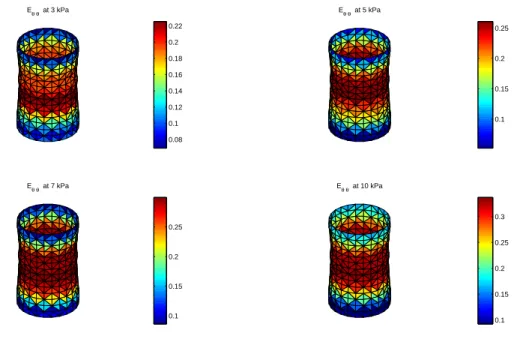
Eθθ at 3 kPa Eθθ at 5 kPa Eθθ at 7 kPa Eθθ at 10 kPa 0.08 0.1 0.12 0.14 0.16 0.18 0.2 0.22 0.1 0.15 0.2 0.25 0.1 0.15 0.2 0.25 0.1 0.15 0.2 0.25 0.3
Figure 3: Plot of the circumferential components of the Green-Lagrange strain tensor for different values of p. The plot is displayed in the undeformed configuration.
σθθ (in MPa) at 3 kPa σθθ (in MPa) at 5 kPa
σθθ (in MPa) at 7 kPa σθθ (in MPa) at 10 kPa
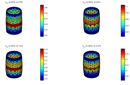
0.01 0.02 0.03 0.04 0.05 0.06 0.02 0.04 0.06 0.08 0.1 0.02 0.04 0.06 0.08 0.1 0.12 0.14 0.16 0.18 0.05 0.1 0.15 0.2 0.25
Figure 4: Plot of the circumferential components of the Cauchy stress tensor for different values of p. The plot is displayed in the deformed configuration. The Cauchy stress are calculated with the Fung model using the identified values reported in Tab.1
0.01 0.015 0.02 0.025
pressure (MPa) with virtual field 1
IVW EVW 0 0.005 0.01 0.015 0.02 0.025 0 5 10 15 20 25 30 pressure (MPa) virtual work
with virtual field 2
IVW EVW
Figure 5: Comparison of the internal and external virtual work for virtual field 1 (a) and virtual field 2 (b) when an anisotropic model is identitied
0.01 0.015 0.02 0.025
pressure (MPa) with virtual field 1
0 0.005 0.01 0.015 0.02 0.025 0 20 40 60 80 100 120 pressure (MPa) virtual work
with virtual field 2
EVW
IVW EVW
Figure 6: Comparison of the internal and external virtual work for virtual field 1 (a) and virtual field 2 (b) when an isotropic model is identitied
0.002 0.004 0.006 0.008 0.01 0.012 0.014 0.016 0.018 0.02
Pressure (MPa)
experimental radii radii obtained by FE
0.1 0.2 0.3 0.4
E11 (a)
experimental stress/strain curve identified Fung model
0 0.1 0.2 0.3 0.4 0.5 0 0.01 0.02 0.03 0.04 0.05 0.06 0.07 0.08 0.09 E22 S 22 (MPa) (b)
experimental stress/strain curve identified Fung model
PSfrag replacements
S11
E11
S22
E22