HAL Id: hal-01365342
https://hal.archives-ouvertes.fr/hal-01365342
Submitted on 13 Sep 2016
HAL is a multi-disciplinary open access
archive for the deposit and dissemination of sci-entific research documents, whether they are pub-lished or not. The documents may come from teaching and research institutions in France or abroad, or from public or private research centers.
L’archive ouverte pluridisciplinaire HAL, est destinée au dépôt et à la diffusion de documents scientifiques de niveau recherche, publiés ou non, émanant des établissements d’enseignement et de recherche français ou étrangers, des laboratoires publics ou privés.
Coupled heat conduction and multiphase change
problem accounting for thermal contact resistance
Daniel Weisz-Patrault
To cite this version:
Daniel Weisz-Patrault. Coupled heat conduction and multiphase change problem accounting for ther-mal contact resistance. International Journal of Heat and Mass Transfer, Elsevier, 2017, 104, pp.595-606. �10.1016/j.ijheatmasstransfer.2016.08.091�. �hal-01365342�
Coupled heat conduction and multiphase change problem
accounting for thermal contact resistance
Daniel Weisz-Patrault
LMS, ´Ecole Polytechnique, CNRS, Universit´e Paris-Saclay, 91128 Palaiseau, France
Abstract
In this paper, heat conduction coupled with multiphase changes are considered in a cylindrical multilayer composite accounting for thermal contact resistance depending on contact pressures and roughness parameters. A numerical simulation is proposed using both analytical develop-ments and numerical computations. The presented modeling strategy relies on an algorithm that alternates between heat conduction accounting for volumetric heat sources and a multi-phase change model based on non-isothermal Avrami’s equation using the isokinetic assump-tion. Applications to coiling process (winding of a steel strip on itself) are considered. Indeed, phase changes determine the microstructure of the final material and are responsible for resid-ual stresses that create flatness defects. A Finite Element modeling is used for validating the presented solution and numerical results are presented and discussed.
Keywords: Multiphase changes, Heat conduction, Analytical solution, Coiling process
1. Introduction
1.1. Heat conduction problem in a multilayer composite
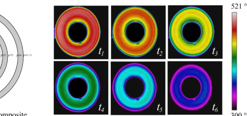
A cylindrical multilayer composite is considered as shown in figure 1a. Contact pressures, that can vanish if contact is not ensured, are known as well as heterogeneous initial temperature
and phase fields. This paper aims at developing a modeling strategy enabling effective
simu-lation of the unsteady heat conduction problem, accounting for multiphase changes that occur during cooling. Since applications to axisymmetric coil cooling problems are considered, a ra-dial model is derived, although the circumferential direction could have been addressed. Heat fluxes along the axial direction are neglected despite the fact that the temperature field slightly evolves along the axial direction because of contact pressure distribution and boundary condi-tions at cylinder edges. Therefore, a one-dimensional problem is obtained and applied several
times at different axial locations. Industrial temperature measurements, recorded with an
in-frared camera during coil cooling, are presented in figure 1b. The axisymmetric assumption is well verified.
(a) Multilayer composite
(b) Axisymmetric coil cooling problem Figure 1: Heat conduction modeling
The heat conduction modeling strategy relies on analytical developments. This choice leads to reasonable computation times that enable parametric studies. Analytical solutions for mul-tilayer composites have already been studied. For instance, the analytical solution of the un-steady heat conduction problem without heat sources in a 1D multilayer composite has been established in plates, cylinders and spheres by De Monte [1, 2]. An extension has been proposed by De Monte [3] for a 2D bi-layer composite in Cartesian coordinates. More recently Singh et al. [4], Jain et al. [5] extended this solution for a cylindrical 2D multilayer composite (radial and circumferential directions) considering time-independent heat sources. The same problem has been solved for spherical configurations by Jain et al. [6]. The radial 1D heat conduction problem for a bi-layer composite has been recently solved by Li and Lai [7] using Laplace transforms. All these works do not consider heat sources or deal with time-independent heat sources. In this paper, a coupling with multiphase change problems is considered, thus time and space dependent heat sources should be taken into account.
Necati ¨Ozıs¸ık [8] obtained a very elegant solution for the 1D heat conduction problem in
multilayer composites (plate, cylinder and sphere) considering time and space dependent heat sources. A compact closed-form solution, very suitable for analytical heat sources, is proposed. However, in this paper heat sources are given numerically as outputs of the multiphase change problem, with a given time and space discretization. It should be noted that a direct numerical
computation of the closed-form solution proposed in [8] would not be efficient in terms of
computation times. Indeed, the latter solution relies for each time t on a primitive denoted
by∫0tg∗n(t′)dt′, where functions g∗n(t′) are defined for each time t′ as a sum of several numerical
integrals over the strip thickness. The time discretization can be very fine, so that phase changes
are correctly described. Since t′ lies between 0 and t the time discretization for the integrand
g∗n(t′) should be even finer and numerical evaluations of the proposed solution are long for the
considered applications. The solution presented in [8] relies on an expansion of heat sources into a series of the form (25). In this paper, an alternative idea is to expand heat sources into time-dependent exponential series by using data fit procedures. The obtained solution
avoids long numerical computations of g∗n(t′) and mainly rely on matrix inversion. One could
have used the closed-form solution in [8] at this point, however calculations are done under the assumption that heat fluxes vanish at the inner radius. The solution could be fairly easily
adapted for a surrounding temperature at the inner radius identical to those at the outer radius, but more significant changes should be made if the surrounding temperature at the inner radius
is different from those at the outer radius. Therefore, the analytical solution derived in the
following enables to consider different surrounding temperatures at inner and outer surfaces.
Mathematical developments rely on quite similar ideas developed in [8] on the one hand and data fit procedures on the other hand.
1.2. Thermal contact resistance
Furthermore, contact pressures between layers are assumed to be known. Therefore, ther-mal contact resistance can be evaluated depending on roughness profiles. All previously cited analytical solutions deal with continuous temperature and heat flux through each interface, which corresponds to perfect thermal contact. Indeed, orthogonality relations that are used to fulfill the initial condition do not hold if thermal contact resistances are introduced. In this
pa-per, this difficulty is overcome by assuming perfect contact conditions, however thin insulating
air gaps between steel layers are introduced, in order to model an equivalent thermal contact resistance. The appropriate air gap thickness is determined as a function of thermal contact resistance by ensuring that the heat flux flowing through the imperfect interface is the same as the average heat flux flowing through the equivalent air gap. The macroscopic temperature discontinuity at the interface that defines thermal contact resistance is presented in principle in figure 2a. The modeling strategy relying on temperature and flux continuities, thin insulating air gaps are introduced in order to smooth interface discontinuities without pretending a better description of the real contact. Indeed, the latter smoothing is rather artificial and relies com-pletely on established thermal contact resistance that characterizes stochastic properties of real contact topology.
Determination of thermal contact resistance between rough surfaces has been intensively studied. Kaza [9] presents an interesting review of the field and based on contact theories and experiments a thermal contact resistance that depends on roughness parameters and contact pressure is proposed. This latter thermal contact resistance is used in this paper. The real contact area is only a small proportion of the nominal contact area according to roughness of both surfaces. There remain asperities that are filled usually with a gas or a liquid if con-tact is lubricated. Early papers of Shlykov and Ganin [10] and Cooper et al. [11] describe a calculation method of thermal contact resistance for steel, depending on contact pressure and roughness. Two thermal contact resistances considered as parallel resistances are identified, namely constriction resistance and resistance of asperities. On the one hand, constriction re-sistance describes the fact that the heat flux narrows towards the actual contact spots. On the other hand, resistance of asperities represents the insulation due to the fluid that lies in the as-perities. These classical contributions are represented in figure 2b. Models based on stochastic treatments of asperities have been developed by Miki´c [12, 13] and take the interface defor-mation into account. For lubricated contacts on can mention more recent models developed by Hamasaiid et al. [14] and Yuan et al. [15] giving analytical predictions of thermal contact resistance at liquid-solid interfaces. Most models have been validated experimentally for low contact pressures, Fieberg and Kneer [16] proposed an experimental setup in order to measure thermal contact resistance under higher pressure and temperature conditions.
(a) Temperature at the interface
(b) Constriction resistance and asperities
Figure 2: Thermal contact resistance
1.3. Multiphase change
In this paper, phase changes that occur during cooling are considered. Solid iron has only
two possible phases, namely austenite or (γ) phase that is stable at high temperature and
cor-responds to a face-centered cubic lattice (fcc) and ferrite or (α) phase that is stable at room
temperature and corresponds to a body-centered cubic lattice (bcc). Steel being an alloy of iron and carbon (and other chemical additives such as manganese, chlorine etc...) more complicated patterns can be formed. A schematic phase diagram Fe-C is presented in figure 3. Several
con-figurations are therefore identified as different steel phases such as austenite, ferrite, pearlite,
bainite and martensite. Schematically during cooling, austenite is transformed into ferrite. Car-bon solubility in ferrite being very small, carCar-bon atoms migrate towards austenite and carCar-bon concentration increases. When austenite is saturated in carbon atoms, the latter precipitate and
form cementite (Fe3C). Thus, pearlite then bainite are formed, depending on geometrical
pat-terns between ferrite and cementite. If a characteristic temperature MS is reached, martensite can be produced from residual austenite. It basically consists in a fast transformation without carbon migration. All these phases are considered in the following, however this paper does
not focus on their metallurgical or mechanical aspects. The different stages through which a
phase change occur are classically nucleation, growth and coalescence. A review of this field is given for instance by Pan [17]. In this paper, only the overall kinetics of the phase transforma-tion, giving the transformation rate, is needed. Avrami [18] gives the well-known fundamental
equation (31) predicting transformation kinetics for diffusive transformations under isothermal
assumption. The solution is based on the idea that small germ nuclei of the new phase are pre-existing and can be transformed into active growth nuclei or be swallowed by growing grains of the new phase. Statistical treatments are used to compute the overlapping volume between
different growing grains. Avrami [18] also defines the isokinetic range as the assumption that
the growth rate is proportional to the probability of creating active growth nuclei from germ nuclei. For non-isothermal conditions, the isokinetic assumption has been extended by Cahn [19] leading to equation (32) as reviewed for instance by Christian [20]. On the other hand, the
diffusionless martensite transformation is modeled using the work of Koistinen and Marburger
the main issue being to propose an efficient modeling strategy to couple heat conduction and multiphase change problems.
Figure 3: Phase diagram Fe-C
1.4. Applications
Applications to coiling process are considered. This consists in winding under tension a steel strip on a cylindrical mandrel. This process is very commonly used in the steel making industry for storage. Residual stress issues are significant during coiling process. Indeed, plas-tic deformations and phase changes occur during the winding of the strip on itself. Based on previous works [22, 23], a mechanical model has been recently proposed by Weisz-Patrault et al. [24] in order to solve (with reasonable computation times) this highly nonlinear prob-lem, where rough contacts of the strip on itself, elastic-plastic behavior and large rotations are involved. The final residual stress profile is one of the main outputs. One can extract from this latter model both geometry and contact pressures in the coil that are assumed to be known in the present paper. Phase changes aspects during the coil cooling are also significant with respect to residual stress issues. Indeed, when the final coil stored in order to cool down, phase changes occur modifying the residual stress profile. A very few attempts to a better understand-ing of this part of the process have been published. For instance Park et al. [25], Saboonchi and Hassanpour [26], Karlberg [27] proposed numerical models dedicated to the heat conduction problem in the coil without phase transformation. A coupling with thermal and phase change problems is proposed for coil annealing by Mehta and Sahay [28].
1.5. Organization of the paper
The paper is organized as follows. In section 2 heat conduction is solved analytically, in a cylindrical multilayer composite accounting for known time-dependent heat sources. Suitable series expansion is proposed for heat sources, so that an analytical particular solution can be found. Multiphase changes are addressed in section 3, assuming a known temperature field. A summary of the coupling algorithm is given in section 4. In section 5, a brief and simple model enables to fix air gaps thicknesses in order to take into account thermal contact resistance.
In section 6, a Finite Element model is carried out, in order to validate the exactness of the proposed solution. Eventually, the model is tested and results are discussed in section 7. 2. Heat conduction problem
Assuming multiphase changes, heat sources due to enthalpy changes should be taken into account, therefore the unsteady heat equation is:
∂2T(i) tot ∂r2 + 1 r ∂T(i) tot ∂r − 1 D(i) ∂T(i) tot ∂t = − Np ∑ p=1 ∆Hp(T ) λ(i) X˙ (i) p (1)
where as a general rule in the following, the superscript (i) is related to the i-th layer, n+1 is the
total number of layers, Ttot(i) is the total temperature in the i-th layer, D(i) the thermal diffusivity,
λ(i) the thermal conductivity, N
pthe number of produced phases, ∆Hpthe temperature
depen-dent enthalpy change associated to the p-th phase change and ˙X(i)p the p-th phase proportion rate.
This partial differential equation is nonlinear because of the temperature dependent right-side
term. However thermal conductivity and diffusivity are assumed to be temperature
indepen-dent, so that the homogenous partial differential equation is linear. The strategy to deal with
non-linearity relies on the coupling scheme that consists in alternating heat conduction prob-lem with known heat sources and multiphase change probprob-lem with known temperature field. Iterations (starting from an initial guess) are carried out to capture the temperature dependence of heat sources. The temperature dependent right-side term is then replaced by known time and space dependent heat sources and the inhomogeneous equation becomes linear. Therefore, the
total solution can be decomposed into an homogenous solution T(i)of the heat equation without
right-side term (3) and a particular solution bT(i):
Ttot(i) = T(i)+ bT(i) (2)
2.1. Homogenous heat equation
The homogenous heat equation is written as follows: ∂2T(i) ∂r2 + 1 r ∂T(i) ∂r − 1 D(i) ∂T(i) ∂t = 0 (3)
By using separation of variables techniques considering time and space dependencies, time dependency only and space dependency only, an analytical solution can be written as follows:
T(i)(r, t) = Nk ∑ k=1 [ Θ(i) k J0 ( βk √ D(i)r ) + Θ e (i) k Y0 ( βk √ D(i)r )] exp(−β2kt)+ Γ(i)ln ( r r(i) ) + Γ e (i) (4)
where J0 and Y0 are the 0-order Bessel functions of the first and second kind respectively, βk
are unknown eigenvalues andΘ(i)k , Θ
e
(i)
k , Γ
(i), Γ
e
(i)are unknown coefficients. Boundary conditions
are temperature and heat flux continuities through all interfaces and heat flux conditions using
heat transfer coefficients at both inner and outer surfaces. Thus (for i ∈ {0, ..., n − 1}):
[0] : λ(0)∂T (0) ∂r (r(0), t) = H(0) ( T(0)(r(0), t) − Tint ) [i]T : T(i)(r(i+1), t) = T(i+1)(r(i+1), t) [i]H : λ(i) ∂T(i) ∂r (r(i+1), t) = λ(i+1) ∂T(i+1) ∂r (r(i+1), t) [n] : λ(n)∂T (n) ∂r (r(n+1), t) = −H(n+1) ( T(n)(r(n+1), t) − Text ) (5)
Of course boundary conditions of the particular solution bT(i) should be consistent with (5) so
that the total problem verifies also (5) that is to say that bT(i)should also verify [i]
T and [i]Hbut
the surrounding temperature should vanish in conditions [0] and [n] of (5) as detailed in (19). By plugging (4) into (5) it is obtained on the one hand:
Θ(0) k [ λ(0) βk √ D(0)J ′ 0 ( βk √ D(0)r (0) ) − H(0)J 0 ( βk √ D(0)r (0) )] + Θ e (0) k [ λ(0) βk √ D(0)Y ′ 0 ( βk √ D(0)r (0) ) − H(0)Y 0 ( βk √ D(0)r (0) )] = 0 Θ(i) k J0 ( βk √ D(i)r (i+1) ) + Θ e (i) k Y0 ( βk √ D(i)r (i+1) ) −Θ(i+1) k J0 ( βk √ D(i+1)r (i+1) ) − Θ e(i+1)k Y0 ( βk √ D(i+1)r (i+1) ) = 0 Θ(i) k λ (i) βk √ D(i)J ′ 0 ( βk √ D(i)r (i+1) ) + Θ e (i) k λ (i) βk √ D(i)Y ′ 0 ( βk √ D(i)r (i+1) ) −Θ(i+1) k λ (i+1) βk √ D(i+1)J ′ 0 ( βk √ D(i+1)r (i+1) ) − Θ e(i+1)k λ (i+1) βk √ D(i+1)Y ′ 0 ( βk √ D(i+1)r (i+1) ) = 0 Θ(n) k [ λ(n) βk √ D(n)J ′ 0 ( βk √ D(n)r (n+1) ) + H(n+1)J 0 ( βk √ D(n)r (n+1) )] + Θ e (n) k [ λ(n) βk √ D(n)Y ′ 0 ( βk √ D(n)r (n+1) ) + H(n+1)Y 0 ( βk √ D(n)r (n+1) )] = 0 (6)
and on the other hand: Γ(0)λ(0) r(0) − Γe (0) H(0) = −H(0)Tint Γ(i)ln ( r(i+1) r(i) ) + Γ e (i)− Γ e (i+1)= 0
Γ(i)λ(i)− Γ(i+1)λ(i+1)= 0
Γ(n) ( λ(n) r(n+1) + H (n+1)ln ( r(n+1) r(n) )) + H(n+1)Γ e(n)= H(n+1)Text (7)
From both systems (6) and (7) one obtains:
Hk.Θk = 0 (8) h.Γ = F (9) where: Θk = ( Θ(0) k , Θe (0) k , · · · , Θ (n) k , Θe (n) k )T Γ = (Γ(0), Γ e(0), · · · , Γ(n), Γe(n) )T F= (−H(0)T int, 0, · · · , 0, H(n+1)Text )T (10)
where Hk (that depends explicitly onβk) and h are matrices of size 2(n+ 1) × 2(n + 1) clearly
defined by (6) and (7). These matrices are of the form:
H1,1 H1,2 0 0 0 0 · · · 0 0 0 0 H2,1 H2,2 −H2,3 −H2,4 0 0 · · · 0 0 0 0 H3,1 H3,2 −H3,3 −H3,4 0 0 · · · 0 0 0 0 0 0 H4,3 H4,4 −H4,5 −H4,6 · · · 0 0 0 0 0 0 H5,3 H5,4 −H5,5 −H5,6 · · · 0 0 0 0 ... 0 0 0 0 0 0 · · · H2n,2n−1 H2n,2n −H2n,2n+1 −H2n,2n+2 0 0 0 0 0 0 · · · H2n+1,2n−1 H2n+1,2n −H2n+1,2n+1 −H2n+1,2n+2 0 0 0 0 0 0 · · · 0 0 H2n+2,2n+1 H2n+2,2n+2 (11)
The system (9) can be solved easily, since h does not depend on eigenvalues and is invertible. Conditioning issues may arise because of very severe contrasts with respect to layer thick-nesses and material properties. Indeed, applications to steel layers with very thin air gaps are considered. This can be regularized by increasing slightly the thermal conductivity of air gaps (it should remain insulating compared with steel). Therefore, the equivalent air gap thickness
derived in section 5 increases, reducing both geometrical and material contrasts. Thus, coe
ffi-cientsΓ(i) andΓ
e
(i) reads:
Γ = h−1.F (12)
However, a non-trivial solution of (8) can be found if and only if the matrix determinant
van-ishes. Therefore eigenvaluesβk are determined by finding positive successive roots of the
de-terminant of the matrix Hk. The higher Nk is chosen and better the initial condition is verified.
The rank of the matrix Hkis 2n+1, therefore the solution set is a one-dimensional vector space
that can be parametrized byΘ(0)k considered as a right-side term. The last equation of (6) being
automatically verified, the system (8) reduces to (for i∈ {0, ..., n}):
{ Θ(i) k = Θ (0) k α (i) k Θ e (i) k = Θ (0) k αe (i) k (13) where: α (0) k = 1 α e (0) k = − H1,1 H1,2 (14)
and where the following recursive formula holds (for i∈ {0, ..., n − 1}):
( α(i+1) k α e (i+1) k ) = ( H2i+2,2i+3 H2i+2,2i+4 H2i+3,2i+3 H2i+3,2i+4 )−1 . ( H2i+2,2i+1 H2i+2,2i+2 H2i+3,2i+1 H2i+3,2i+2 ) . ( α(i) k α e (i) k ) (15) Therefore the temperature field reduces to:
T(i)(r, t) = Nk ∑ k=1 Θ(0) k [ α(i) k J0 ( βk √ D(i)r ) + α e (i) k Y0 ( βk √ D(i)r )] exp(−β2kt)+ Γ(i)ln ( r r(i) ) + Γ e (i) (16)
The only remaining unknowns are coefficients Θ(0)k . The determination of these latter coe
ffi-cients is done by using the following initial condition Ttot(i)(r, t = 0) = Tini(r) where Tini(r) is the
2.2. Particular solution
The particular solution bT(i) verifies the heat equation (1) accounting for the right-side term.
Phase proportion rates ˙X(i)p (r, t) are obtained numerically in section 3. An analytic form is
needed for the heat equation. Therefore, an expansion into decreasing exponential series is used: −∆Hp(T ) λ(i) X˙ (i) p (r, t) = b Nk ∑ k=1 χ(i) p,k(r) exp ( −bβ2 kt ) + χ(i) p,0(r) (17)
Eigenvalues are arbitrarily chosen such as the data fit procedure is accurate and such as bβk , βk
so that the associated matrix is well conditioned. This new set of eigenvalues are not roots of
any equation and does not cost additional computation time. In this paper bβk are chosen in the
middle of successive βk. Coefficients χ(i)p,k(r) are computed numerically using data fit
proce-dures. It is possible to deal with the r-dependance by using specific orthogonal basis functions presented in Appendix A. However technicalities can be avoided by considering that phase changes are homogenous in each steel layer which is rather well verified considering that steel layers are quite thin (1 or 2 mm). This assumption also enables to avoid a discretization along the radial direction for the multiphase change model presented in section 3. Therefore, in the following, the r-dependance is discarded but a more general solution is addressed in Appendix A. Moreover it should be noted that the analytical form (17) is only an approximation of the heat source because of the data fit procedure. By using separation of variables techniques con-sidering time and space dependencies, time dependency only and space dependency only, a particular solution can be written as follows:
b T(i)(r, t) = b Nk ∑ k=1 bΘ(i) k J0 bβk √ D(i)r + bΘe(i) k Y0 bβk √ D(i)r +∑Np p=1 χ(i) p,k D(i) bβ2 k exp(−bβ2 kt ) +bΓ(i)ln( r r(i) ) + bΓ e (i) + χ (i) p,0 4 r 2 (18)
where bΘ(i)k and bΘ
e
(i)
k are unknown. It should be noted that most parts of the latter form (18) are
solutions of the homogenous heat conduction problem, only terms involvingχ(i)p,k are truly
inho-mogeneous solutions. The particular solution should verify the following boundary conditions
(for i∈ {0, ..., n − 1}): [0] : λ(0)∂bT (0) ∂r (r(0), t) = H(0)Tb(0)(r(0), t) [i]T : bT(i)(r(i+1), t) = bT(i+1)(r(i+1), t) [i]H : λ(i)∂bT (i) ∂r (r(i+1), t) = λ(i+1) ∂bT(i+1) ∂r (r(i+1), t) [n] : λ(n)∂bT (n) ∂r (r(n+1), t) = −H(n+1)bT(n)(r(n+1), t) (19)
Boundary conditions (19) can be written as follows: b
where: bΘk = ( b Θ(0) k , bΘe (0) k , · · · , dΘ(n)k, bΘe (n) k )T bΓ =(bΓ(0),bΓ e (0) , · · · , cΓ(n),bΓ e (n))T (21) and where: bFk= H(0) Np ∑ p=1 χ(0) p,k D(0) bβ2 k ... Np ∑ p=1 χ(i+1)p,k D(i+1) bβ2 k − χ(i) p,k D(i) bβ2 k 0 ... −H(n+1) Np ∑ p=1 χ(n) p,k D(n) bβ2 k and bF= Np ∑ p=1 χ(0) p,0 2 r (0) ( H(0)r (0) 2 − λ (0) ) ... Np ∑ p=1 χ(i+1) p,0 − χ (i) p,0 4 ( r(i+1))2 Np ∑ p=1 λ(i+1)χ(i+1) p,0 − λ(i)χ (i) p,0 2 r (i+1) ... − Np ∑ p=1 χ(n) p,0r(n+1) 2 ( H(n+1)r (n+1) 2 + λ (n) ) (22)
Eventually bΘk and bΓ are determined easily by inverting matrices bHk and h. Thus:
b
Θk = bH
−1
k .bFk and bΓ = h−1.bF (23)
2.3. Initial condition
The initial condition Ttot(i)(r, t = 0) = Tini(r) is finally used in order to determine the only
remaining unknown coefficients Θ(0)k . This process relies on a particular orthogonality relation
related to the following scalar product: ⟨ f1, f2⟩ = n ∑ i=0 λ(i) D(i) ∫ r(i+1) r(i) r f1(r) f2(r)dr (24)
Consider the following basis functions defined on the whole multilayer composite: fk(r) = α(i)k J0 ( βk √ D(i)r ) + α e (i) k Y0 ( βk √ D(i)r ) with r ∈[r(i), r(i+1)] (25)
Therefore, the following orthogonality relation holds as demonstrated by De Monte [2]: ⟨ fk, fl⟩ =
{
0 if k, l
Mk > 0 if k = l
(26)
The basis functions ( fk)k∈{1,··· ,Nk}form an orthogonal basis with respect to the latter scalar
prod-uct. Therefore coefficients (Θ(0)k )
k∈{1,··· ,Nk} are determined by an orthogonal projection of the
initial condition on the orthogonal basis. More precisely, the initial condition reads:
Nk ∑ k=1 Θ(0) k [ α(i) k J0 ( βk √ D(i)r ) + α e (i) k Y0 ( βk √ D(i)r )] + Γ(i) ln ( r r(i) ) + Γ e (i)+ b
Hence: Nk ∑ k=1 Θ(0) k fk(r)= fini(r) (28)
where finiis defined on the whole multilayer composite as follows:
fini(r)= Tini(i)(r)− Γ(i)ln
( r r(i) ) − Γ e (i)− b
T(i)(r, t = 0) with r ∈[r(i), r(i+1)] (29)
Therefore, following coefficients are found:
Θ(0)
k =
⟨ fini, fk⟩
⟨ fk, fk⟩
(30)
3. Multiphase change problem
As described in section 1.3, each phase transformation occur within a temperature range.
Austenite is stable above Ae3. Ferrite is formed between Ae3 and Ae1 and the equilibrium
phase proportion between austenite and ferrite can be evaluated by using the lever rule on the
thermodynamic equilibrium phase diagram. Pearlite is formed between Ae1 and BS, bainite
is then formed between BS and MS, and martensite is formed below MS. Ferrite, pearlite, bainite and martensite are formed from retained austenite. Thus, when all austenite has been consumed, phase transformation stops. The classical equation that describes the overall phase transformation kinetics under isothermal assumption proposed by Avrami [18] is written as
follows (for p= 1, 2, 3 i.e., ferrite, pearlite and bainite):
Xisop (t)= 1 − exp(−kp(T )tnp
)
(31)
where the superscript iso means isotherm. Consider a non-isotherm path given by t′ 7→ T(t′).
Let t be a fixed time and t′ be any time in the interval [0, t]. The phase proportion produced
with the non-isothermal condition during the time interval [0, t] is denoted by Xp(t). Let tiso
de-notes the time that would be necessary to produce the same phase proportion under isothermal
assumption with the following constant temperature T∗ = T(t′) (it depends explicitly on T (t′)
but for sake of conciseness the notation is kept simple). Thus Xiso
p (tiso)= Xp(t). Using (31) one
can write: tiso = −ln ( 1− Xp(t) ) kp(T (t′)) 1 np (32) The isokinetic assumption enables to write:
∫ t
0
dt′ tiso
= 1 (33)
By using (32) and (33) one obtains:
Xp(t)= 1 − exp ( − [∫ t 0 kp(T (t′)) 1 npdt′ ]np) (34) The phase proportion rate is calculated as follows:
˙ Xp(t) = npkp(T (t)) 1 np [∫ t 0 kp(T (t′)) 1 npdt′ ]np−1 exp ( − [∫ t 0 kp(T (t′)) 1 npdt′ ]np) (35)
For martensite transformation (i.e., p = 4) the phase proportion is calculated as proposed by Koistinen and Marburger [21]:
X4(t)= Xra(t)
[
1− exp (−α (T − MS))] (36)
where Xrais the retained austenite andα a constant parameter set to 0.01 in this paper.
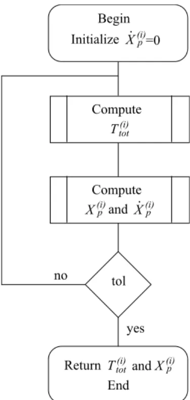
4. Coupling
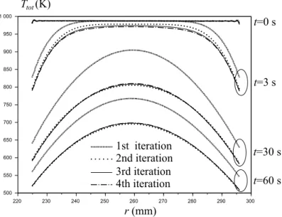
In this paper, the coupling scheme consists simply on alternating both the heat conduction problem with known phase proportion rates and the multiphase change problem with known temperature field. The alternating coupling algorithm is simply depicted in figure 4. Conver-gence is tested on the temperature field and the tolerance is set to 5 K. The algorithm begins with zero phase proportion rates (i.e., no heat source). A first temperature estimation is pro-duced and the multiphase change problem is carried out on this basis, giving the first estimation of heat sources. This scheme is repeated until convergence. No mathematical proof of conver-gence is broached in this paper. But practically, for the present coupled problem, this procedure converges within a very few iterations as shown for instance in figure 5 that is computed from the practical example presented in section 7.
Figure 5: Convergence at Z= 0
5. Equivalent air gap thickness
As detailed in section 1.2, thermal contact resistance is modeled by introducing air gaps between steel layers. Therefore, the solution derived in section 2, that relies on temperature and heat flux continuities through each interface, can be used by alternating steel and thin air layers. The equivalent air gap thickness is determined by ensuring that the average heat
flux through the air gap matches the heat flux at the imperfect steel/steel interface modeled by
thermal contact resistance. Thermal contact resistance is defined by H that depends on contact pressure and roughness parameters. The heat flux at the imperfect interface is classically:
Q= H (T2(t)− T1(t)) (37)
where T1(t) and T2(t) are the temperatures at lower and upper surfaces of the interface as
de-picted in figure 6. The equivalent air gap thickness denoted by th is defined as shown in figure 6,
that is to say that temperatures at lower and upper surfaces of the air gap are also T1(t) and T2(t).
In addition, temperature and heat flux continuities are ensured. Consider that T1(t) and T2(t)
can be written as follows (for j= 1 or 2):
Tj(t) = ∫ +∞ 0 T ej(β) exp ( −β2 t)dβ + T0j (38)
Consider Ta, Da andλa the temperature , thermal diffusivity and thermal conductivity in the
air gap1. A simple equivalent thickness is found by solving the heat conduction problem in
Cartesian coordinates: ∂2T a ∂x2 = 1 Da ∂Ta ∂t (39)
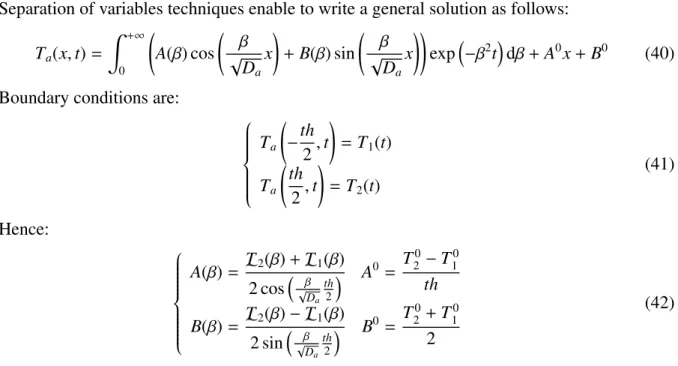
Separation of variables techniques enable to write a general solution as follows: Ta(x, t) = ∫ +∞ 0 ( A(β) cos ( β √ Da x ) + B(β) sin ( β √ Da x )) exp(−β2t)dβ + A0x+ B0 (40)
Boundary conditions are:
Ta ( −th 2, t ) = T1(t) Ta ( th 2, t ) = T2(t) (41) Hence: A(β) = Te2(β) + Te1(β) 2 cos(√β Da th 2 ) A0= T 0 2 − T 0 1 th B(β) = Te2(β) − Te1(β) 2 sin(√β Da th 2 ) B0= T 0 2 + T 0 1 2 (42)
The equivalent air gap thickness is determined by ensuring that the average heat flux through the air gap matches the heat flux at the imperfect interface defined by (37), therefore:
H(T e2(β) − T e1(β) ) = λa th β √ Da ∫ th 2 −th 2 ( −A(β) sin ( β √ Da x ) + B(β) cos ( β √ Da x )) dx = 2λaB(β) sin ( β √ Da th 2 ) th = λa ( T e2(β) − T e1(β) ) th H(T20− T10)= λa th ∫ th 2 −th 2 A0dx= λaA0 = λa ( T0 2 − T 0 1 ) th (43)
Thus, the equivalent air gap thickness is:
th= λa
H (44)
In this paper, thermal contact resistance is extracted from the work of Kaza [9] but other formulations are also possible:
H = λs Rq 2.16 ( P 3.3σY+ P )0.51 + 0.36λa λs (45)
where λs and λa are thermal conductivities of steel and air respectively, P is the local
con-tact pressure, σY the yield stress and Rq the quadratic roughness parameter (average high of
asperities). 6. Validation
In this section, exactness of the analytical solution developed in section 2 (considering the particular solution related to heat sources) is demonstrated by comparing results with a Finite Element model. Thus, an axisymmetric composite, alternating 2 mm thick steel layers
with 5µm thick air layers, is modeled using the freeware Cast3m (http://www-cast3m.cea.fr/).
Details are listed in table 1. Heat sources are directly imposed in steel layers as a known
function P(r, t) in W.mm−3corresponding to∆HpX˙(i)p in (1):
P(r, t) = 0.5 × t(t − 2.5) × (r − 200)(r − 220)/100 (46)
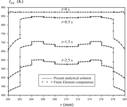
Thus, the coupling problem consisting in computing the heat source as a function of the previ-ous temperature field estimation is not reproduced by FEM. Here, only the analytical solution that gives the temperature field for a known heat source is validated. Validation of the coupling procedure has been done simply by showing convergence within a very few iterations. Com-parison is presented in figure 7 and perfect agreement is observed (it should be mentioned that only half of the Finite Element points are drawn for clarity reasons).
Table 1: Comparison parameters
Steel Air gap
Number of layers 10 9 Thickness (mm) 2 0.005 Thermal conductivity (J.s−1.mm−1.K−1) 50× 10−3 0.026 × 10⁻³ Density (g.mm−3) 7850× 10−6 1.293 × 10⁻⁶ Heat capacity (J.g−1.K−1) 0.5308 1.0054 Thermal diffusivity (mm2.s−1) 12 20
Figure 7: Comparison with FEM
7. First numerical results
Phase change temperatures Ae3, Ae1, BS and MS have been extracted from Lee et al. [29].
Parameters kp and np in the multiphase change problem described in section multiphase have
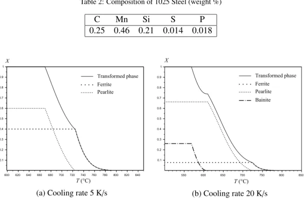
been extracted from Hawbolt et al. [30] for austenite to ferrite and austenite to pearlite trans-formations for a 1025 steel whose composition is listed in table 2. For austenite to bainite transformation, parameters have been extracted from Han et al. [31]. Continuous cooling tests
presented in figure 8 have been carried out at two different cooling rates, namely 5 K/s and
20 K/s. Enthalpy changes during phase transformation are in general temperature dependent.
But for the following example constant values are chosen and give an order of magnitude and do not represent a specific steel. For austenite to ferrite, pearlite and bainite
transfor-mations ∆Hp = −0.4 J.mm−3 (p = 1, 2, 3) and for austenite to martensite transformation
∆H4 = −0.3 J.mm−3.
In the previous paper of Weisz-Patrault et al. [24], the coiling process has been modeled
and 70 wraps have been computed considering a yield stressσY = 600 MPa and a roughness
parameter Rq= 5 µm. Contact pressures and final geometry are extracted and used as inputs for
the present study. A simple elastic calculation is done to simulate that the mandrel is removed, applying on the coil internal surface the opposite contact pressure between the mandrel and the first layer. Resulting contact pressures along the radial direction of the coil are presented in figure 9 for several axial positions. The final geometry is obtained by introducing air gaps between all steel layers according to (44) and (45). When contact pressure vanishes, surfaces are not in contact and then the real air gap is considered. Moreover, the initial temperature
is set to 987 K and the surrounding temperature is 293.15 K. Heat transfer coefficients are
Table 2: Composition of 1025 Steel (weight %)
C Mn Si S P
0.25 0.46 0.21 0.014 0.018
(a) Cooling rate 5 K/s (b) Cooling rate 20 K/s
Figure 8: Continuous cooling test
Figure 9: Contact pressure at different axial positions
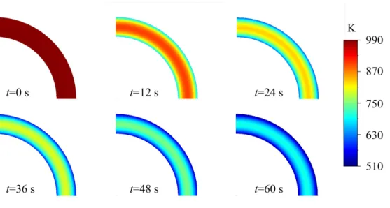
Temperature maps are presented in figure 10. Since the coil is cooled by internal and exter-nal surfaces, the center cools down much slower than near boundaries. The initial temperature
being slightly lower than Ae1 (pearlite start temperature), pearlite then bainite are produced
without producing ferrite. All austenite has been consumed therefore no martensite can be formed when the temperature reaches the martensite temperature start MS. Phase proportion maps are presented in figures 11a and 11b. The time scale has been chosen so that evolutions are visible. It should be noticed that the amount of formed pearlite is more significant at the center than near the internal and external surfaces because the temperature range where pearlite
maximum phase proportion of pearlite is not at the center. This is due to phase transformation kinetics. Indeed, phase transformation is slower when the temperature is maintained near the start temperature of the transformation. When the temperature goes down to the end tempera-ture of the transformation (which is the start temperatempera-ture of the following transformation) there is an acceleration of the phase transformation. Thus, since the center is maintained longer to higher temperature, pearlite transformation is slower is this region. Bainite is mainly formed near the internal and external surfaces where cooling is faster. Temperatures near boundaries are rapidly less than the bainite temperature start BS.
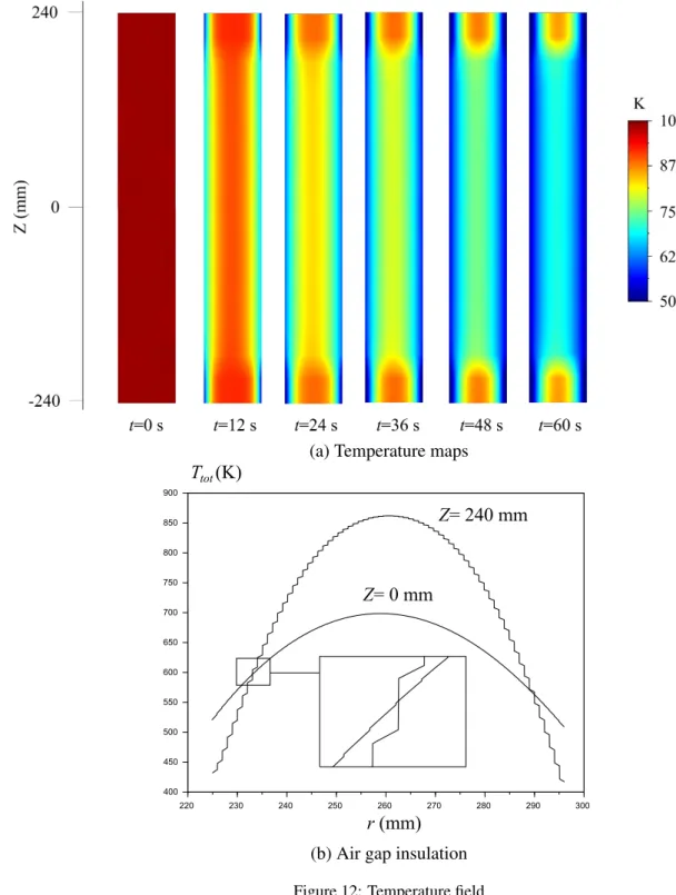
Contact pressures evolve along the axial direction. Temperature maps (along radial and axial directions) are presented in figure 12a. The problem being axisymmetric, these maps are
sufficient to represent the 3D temperature field. Contact pressures increase from the edges to
the coil center (i.e., Z = 0). Thus, globally the central zone cools down faster than the edges
because of thinner air gaps. However, it should be noticed that internal and external surfaces cool down faster at the edges than near the coil center. Indeed, the air gaps being much larger at the edges, first and last layers are insulated from the hot central core. The insulation due to
the air gaps can be observed in figure 12b where the temperature field at t = 60 s is depicted
at Z = 0 mm where contact pressures ensure good conductivity and at Z = 240 mm where
contact is lost between each layer. (It should be mentioned that Weisz-Patrault et al. [24] modeled a 1500 mm long coil. Here only a 480 mm long sub-part of the coil has been modeled
because contact is lost from Z = ±240 mm to Z = ±750 mm leading to similar results as for
Z = ±240 mm.)
(a) Pearlite phase proportion map at Z = 0
(b) Bainite phase proportion map at Z = 0 Figure 11: Phase proportion maps
(a) Temperature maps
(b) Air gap insulation Figure 12: Temperature field
8. Conclusion
Heat conduction problem coupled with multiphase changes have been solved in a cylin-drical multilayer composite accounting for thermal contact resistance depending on contact pressures and roughness. An analytical solution has been proposed, taking into account temper-ature dependent heat sources. The multiphase change problem is solved using classic Avrami’s equation using the isokinetic assumption, in order to deal with non-isothermal conditions. Val-idation has been carried out using a Finite Element simulation. Outputs consist in temperature and phase fields during cooling. Contact pressure distribution and thermal contact resistance
have been taken into account. Significant effects have been found. This coupled problem
com-pletes previous works on coiling process and aims at estimating residual stresses. Therefore, subsequent works should develop the mechanical counterpart of the presented model.
Acknowledgment
The author is very grateful to Alain Ehrlacher (Laboratoire Navier, CNRS, ´Ecole Ponts
ParisTech) and to Nicolas Legrand (ArcelorMittal Global Research & Development East Chicago) for their ideas and their help.
Appendix A. Solution for r-dependent right side terms
This appendix presents a particular solution of the following non-homogeneous partial derivative equation: ∂2Tb(i) ∂r2 + 1 r ∂bT(i) ∂r − 1 D(i) ∂bT(i) ∂t = b Nk ∑ k=1 χ(i) k (r) exp ( −bβ2 kt ) (A.1) Basis functions, orthogonal with respect to the following scalar product, are needed:
⟨g1, g2⟩(i) =
∫ r(i+1) r(i)
rg1(r)g2(r)dr (A.2)
Consider the following basis functions:
g(i)l : [ r(i), r(i+1)] → R r 7→ J0 ( x(i)l r r(i+1) ) Y0 ( x(i)l r (i) r(i+1) ) − J0 ( x(i)l r (i) r(i+1) ) Y0 ( x(i)l r r(i+1) ) (A.3) where (x(i)l ) l∈{1,··· ,bNl}
are successive roots of x 7→ J0(x) Y0
( xrr(i(i)+1) ) − J0 ( xrr(i(i)+1) ) Y0(x). Then, it
should be noted that g(i)l vanishes at r(i) and r(i+1). One can prove the following orthogonality
properties: ⟨ g(i)l , g(i)m⟩ (i) = { 0 if k, l Ml(i) > 0 if l = m (A.4)
Since functions g(i)l (r) vanish at r(i) and ri+1) it is convenient to use the orthogonality property
(A.4) not directly onχ(i)k (r) but on auxiliary functions that vanish at r(i)and r(i+1):
ζ(i) k (r) = χ (i) k (r)− ( A(i)k J0 ( r r(i+1) ) + B(i) k Y0 ( r r(i+1) )) (A.5)
where: ( A(i)k B(i)k ) = ( J0 ( r(i) r(i+1) ) Y0 ( r(i) r(i+1) ) J0(1) Y0(1) )−1 . ( χ(i) k (r (i)) χ(i) k (r (i+1)) ) (A.6) Therefore, using orthogonality properties (A.4), it is obtained:
ζ(i) k (r)= b Nl ∑ l=1 ζ(i) k,lg (i) l (r) (A.7) where: ζ(i) k,l = ⟨ ζ(i) k (r), g (i) l (r) ⟩ (i) ⟨ g(i)l (r), g(i)l (r)⟩ (i) (A.8) The right side term of the heat equation (A.1) is written as follows:
b Nk ∑ k=1 χ(i) k (r) exp ( −bβ2 kt ) = b Nk ∑ k=1 A(i) k J0 ( r r(i+1) ) + B(i) k Y0 ( r r(i+1) ) + b Nl ∑ l=1 ζ(i) k,lg (i) l (r) exp(−bβ2 kt ) (A.9)
Using separation of variables, a particular solution can be written as follows: b T(i)(r, t) = b Nk ∑ k=1 bΘ(i) k J0 bβk √ D(i)r + bΘe(i) k Y0 bβk √ D(i)r + bT(i) k (r) exp(−bβ2 kt ) (A.10) where: b Tk(i)(r)= b Nl ∑ l=1 ζ(i) k,l bβk √ D(i) − ( x(i)l r(i+1) )2 g(i)l (r)+ A(i)k J0 ( r r(i+1) ) + B(i) k Y0 ( r r(i+1) ) bβk √ D(i) − ( 1 r(i+1) )2 (A.11) References
[1] F. De Monte, Transient heat conduction in one-dimensional composite slab. a natural analytic approach, International Journal of Heat and Mass Transfer 43 (2000) 3607–3619. [2] F. De Monte, An analytic approach to the unsteady heat conduction processes in one-dimensional composite media, International Journal of Heat and Mass Transfer 45 (2002) 1333–1343.
[3] F. De Monte, Unsteady heat conduction in two-dimensional two slab-shaped regions. exact closed-form solution and results, International Journal of Heat and Mass Transfer 46 (2003) 1455–1469.
[4] S. Singh, P. K. Jain, et al., Analytical solution to transient heat conduction in polar coor-dinates with multiple layers in radial direction, International Journal of Thermal Sciences 47 (2008) 261–273.
[5] P. K. Jain, S. Singh, et al., Analytical solution to transient asymmetric heat conduction in a multilayer annulus, Journal of Heat Transfer 131 (2009) 011304.
[6] P. K. Jain, S. Singh, et al., An exact analytical solution for two-dimensional, unsteady, multilayer heat conduction in spherical coordinates, International Journal of Heat and Mass Transfer 53 (2010) 2133–2142.
[7] M. Li, A. C. Lai, Analytical solution to heat conduction in finite hollow composite cylin-ders with a general boundary condition, International Journal of Heat and Mass Transfer 60 (2013) 549–556.
[8] M. Necati ¨Ozıs¸ık, Boundary value problems of heat conduction, Dover, 1968. 3rd edition
(2002).
[9] G. Kaza, Contribution `a l’´etude de la r´esistance thermique de contact et `a sa mod´elisation
`a travers l’´ecrasement de l’interface tˆole/outil dans la mise en forme `a chaud de tˆoles
d’acier, Ph.D. thesis, Universit´e de Toulouse, Universit´e Toulouse III-Paul Sabatier, 2010. [10] Y. P. Shlykov, Y. A. Ganin, Thermal resistance of metallic contacts, International Journal
of Heat and Mass Transfer 7 (1964) 921–929.
[11] M. Cooper, B. Mikic, M. Yovanovich, Thermal contact conductance, International Journal of Heat and Mass Transfer 12 (1969) 279–300.
[12] B. Miki´c, Thermal constriction resistance due to non-uniform surface conditions; contact resistance at non-uniform interface pressure, International Journal of Heat and Mass Transfer 13 (1970) 1497–1500.
[13] B. Miki´c, Thermal contact conductance; theoretical considerations, International Journal of Heat and Mass Transfer 17 (1974) 205–214.
[14] A. Hamasaiid, M. Dargusch, T. Loulou, G. Dour, A predictive model for the thermal contact resistance at liquid–solid interfaces: analytical developments and validation, In-ternational Journal of Thermal Sciences 50 (2011) 1445–1459.
[15] C. Yuan, B. Duan, L. Li, B. Shang, X. Luo, An improved model for predicting ther-mal contact resistance at liquid–solid interface, International Journal of Heat and Mass Transfer 80 (2015) 398–406.
[16] C. Fieberg, R. Kneer, Determination of thermal contact resistance from transient temper-ature measurements, International Journal of Heat and Mass Transfer 51 (2008) 1017– 1023.
[17] Y.-T. Pan, Measurement and Modelling of Diffusional Transformation of Austenite in
C-Mn Steels, Ph.D. thesis, National Sun Yat-Sen University, 2001.
[18] M. Avrami, Kinetics of phase change. i general theory, The Journal of Chemical Physics 7 (1939) 1103–1112.
[19] J. W. Cahn, The kinetics of grain boundary nucleated reactions, Acta Metallurgica 4 (1956) 449–459.
[20] J. W. Christian, The Theory of Transformations in Metals and Alloys, Pergamon, 1965. 3rd edition (2002).
[21] D. Koistinen, R. Marburger, A general equation prescribing the extent of the austenite-martensite transformation in pure iron-carbon alloys and plain carbon steels, acta metal-lurgica 7 (1959) 59–60.
[22] D. Weisz-Patrault, A. Ehrlacher, N. Legrand, E. Mathey, Non-linear numerical simulation of coiling by elastic finite strain model, Key Engineering Materials 651-653 (2015) 1060– 1065.
[23] D. Weisz-Patrault, A. Ehrlacher, Curvature of an elasto-plastic strip at finite strains: ap-plication to fast simulation of coils, in: 22i`eme Congr`es Franc¸ais de M´ecanique, AFM, Association Franc¸aise de M´ecanique, pp. 1–14.
[24] D. Weisz-Patrault, A. Ehrlacher, N. Legrand, Non-linear simulation of coiling accounting for roughness of contacts and multiplicative elastic-plastic behavior, International Journal of Solids and Structures 94-95 (2016) 1–20.
[25] S.-J. Park, B.-H. Hong, S. C. Baik, K. H. Oh, Finite element analysis of hot rolled coil cooling., ISIJ International 38 (1998) 1262–1269.
[26] A. Saboonchi, S. Hassanpour, Heat transfer analysis of hot-rolled coils in multi-stack storing, Journal of Materials Processing Technology 182 (2007) 101–106.
[27] M. Karlberg, Modelling of the temperature distribution of coiled hot strip products, ISIJ International 51 (2011) 416–422.
[28] R. Mehta, S. S. Sahay, Heat transfer mechanisms and furnace productivity during coil annealing: aluminum vs. steel, Journal of Materials Engineering and Performance 18 (2009) 8–15.
[29] M.-G. Lee, S.-J. Kim, H. N. Han, W. C. Jeong, Implicit finite element formulations for multi-phase transformation in high carbon steel, International Journal of Plasticity 25 (2009) 1726–1758.
[30] E. Hawbolt, B. Chau, J. Brimacombe, Kinetics of austenite-ferrite and austenite-pearlite transformations in a 1025 carbon steel, Metallurgical Transactions A 16 (1985) 565–578. [31] H. N. Han, J. K. Lee, H. J. Kim, Y.-S. Jin, A model for deformation, temperature and phase transformation behavior of steels on run-out table in hot strip mill, Journal of Materials Processing Technology 128 (2002) 216–225.