HAL Id: hal-00834482
https://hal-mines-paristech.archives-ouvertes.fr/hal-00834482
Submitted on 15 Jun 2013
HAL is a multi-disciplinary open access
archive for the deposit and dissemination of
sci-entific research documents, whether they are
pub-lished or not. The documents may come from
teaching and research institutions in France or
abroad, or from public or private research centers.
L’archive ouverte pluridisciplinaire HAL, est
destinée au dépôt et à la diffusion de documents
scientifiques de niveau recherche, publiés ou non,
émanant des établissements d’enseignement et de
recherche français ou étrangers, des laboratoires
publics ou privés.
Semi-Supervised Hyperspectral Image Segmentation
Using Regionalized Stochastic Watershed
Jesus Angulo, Santiago Velasco-Forero
To cite this version:
Jesus Angulo, Santiago Velasco-Forero. Semi-Supervised Hyperspectral Image Segmentation Using
Regionalized Stochastic Watershed. Algorithms and Technologies for Multispectral, Hyperspectral,
and Ultraspectral Imagery XVI, May 2010, Orlando, United States. 12 p., �10.1117/12.850187�.
�hal-00834482�
Semi-supervised hyperspectral image segmentation using
regionalized stochastic watershed
Jes´
us Angulo
aand Santiago Velasco-Forero
a aCMM-Centre de Morphologie Math´
ematique, Math´
ematiques et Syst`
emes, MINES ParisTech;
35, rue Saint-Honor´
e, 77305 Fontainebleau cedex - France
ABSTRACT
Stochastic watershed is a robust method to estimate the probability density function (pdf) of contours of a multi-variate image using MonteCarlo simulations of watersheds from random markers. The aim of this paper is to propose a stochastic watershed-based algorithm for segmenting hyperspectral images using a semi-supervised approach. Starting from a training dataset consisting in a selection of representative pixel vectors of each spectral class of the image, the algorithm calculate for each class a membership probability map (MPM). Then, the MPM of class k is considered as a regionalized density function which is used to simulate the random markers for the MonteCarlo estimation of the pdf of contours of the corresponding class k. This pdf favours the spatial regions of the image spectrally close to the class k. After applying the same technique to each class, a series of pdf are obtained for a single image. Finally, the pdf’s can be segmented hierarchically either separately for each class or after combination, as a single pdf function. In the results, besides the generic spatial-spectral segmentation of hyperspectral images, the interest of the approach is also illustrated for target segmentation.
Keywords: hyperspectral images, semi-supervised segmentation, stochastic watershed, regionalized random germs, probabilistic segmentation
1. INTRODUCTION
Watershed transformation is one of the most powerful tools for image segmentation. Starting from a gradient, the classical paradigm of watershed segmentation consists in determining markers for each region of interest. The markers avoid the over-segmentation (a region is associated to each minimum of the function) and moreover, the watershed is relatively robust to marker position.3 The segmentation by watershed of hyperspectral images
has shown to improve the results of classification in hyperspectral images.15, 16 To deals with some drawbacks of
the classical deterministic watershed, the stochastic watershed1(SW) was introduced to detect and to regularize
the contours which are robust with respect to variations in the segmentation conditions. The initial framework was then extended to multispectral images11 and later, a specific methodology of classification-driven stochastic
watershed for multivariate images such as multi/hyper-spectral images was also proposed.12 More recently, we have also considered in2 a probabilistic multiscale framework for the computation of the probability of contours
using different multiscale frameworks of stochastic watershed.
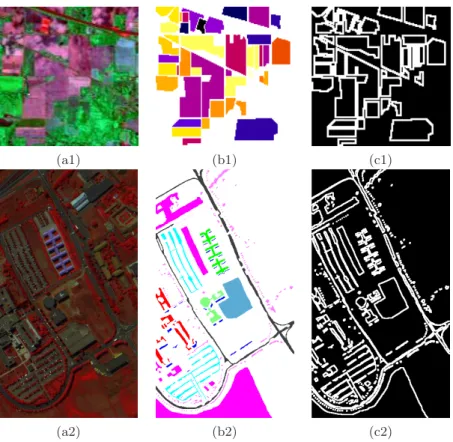
Fig. 1 depicts two standard examples of remote sensing hyperspectral images which will be used in the study. The first dataset is the hyperspectral image of the Indian Pines (200 spectral bands in the 400-2500 nm range, 145x145 pixels), obtained by the AVIRIS sensor. This is a typical example of high spectral resolution image but with a low spatial resolution, which is particularly useful, for instance, in remote sensing agricultural applications. The other dataset is an airbone image, from the ROSIS-3 optical sensor, of the University of Pavia (103 spectral bands of 340x610 pixels). This kind of high spatial resolution image can be typically considered in remote sensing geography or military applications. In the same figure are given, on the one hand, a false colour image with the ground truth pixel classification, and on the other hand, the image of contours of each region of the spectral classification. To be more precise, given a certain set of spectral classes, the pixels belonging to the same spectral class are manually labelled with the same “colour” (the background here is in white). This kind
Further author information: (Send correspondence to J.A. or to S.V.-F.) J. Angulo: E-mail: [email protected]
(a1) (b1) (c1)
(a2) (b2) (c2)
Figure 1. Two standard examples of remote sensing hyperspectral images: (1) “Indian Pines” and (2) “Pavia”. The false colour images (a) are obtained from three significant spectral bands. The spectral classes defined by the ground truth classification are given in images (b): 16 classes for “Indian Pines” and 9 classes for “Pavia” (the background class appears in white). The images (c) represent the contours of the regions associated to the ground truth classification.
of reference is very useful to evaluate the performance of pixel classification algorithms. However, as we observe from both examples, there are many spatial structures which clearly appear on the original images but which are not associated to contours of the spectral classes to be separated, e.g., regions typically associated to the “background” spectral class.
Image segmentation can be considered under two different paradigms: unsupervised and supervised. In unsupervised image segmentation, the aim is to obtain in a reliable way the contours of the most significant spatial/spectral structures. In high spatial resolution images, as the example “Pavia”, there are many com-plex structures at various scales and the definition of a single segmentation is a challenging difficult problem. In supervised image segmentation, some prior information is introduced to help the segmentation procedure. Typically, this prior knowledge corresponds to: i) “markers” for the regions of interest, in the case of interac-tive segmentation; or ii) to a pixel classification in homogenous regions, which are the germs for an automatic segmentation.
Hyperspectral imaging is an active field of image analysis which is usually considered under the supervised paradigm: both the complexity of the data and the typical real-life applications require the construction of training sets of spectra which drive the algorithms of classification, feature extraction, segmentation, etc. In this paper we would like to be coherent with this paradigm, and we use the prior information from a spectral training dataset in order to produce a kind of hyperspectral segmentation using the stochastic watershed-based algorithm. In fact, our method does not include a deterministic classification step of pixels and this is reason why we consider the approach as a semi-supervised segmentation; however our technique is not related to the semi-supervised learning paradigm of classification.5
each spectral class of the image, the algorithm calculate for each class a membership probability map (MPM). Then, the MPM of class k is considered as a regionalized density function which is used to simulate the random markers used in the MonteCarlo estimation of the pdf of contours of the corresponding class k. This pdf favours the spatial regions of the image close spectrally to the class k. After applying the same technique to each class, a series of pdf are obtained for a single image. Finally, the pdf’s can be segmented hierarchically either separately for each class or after combination, as a single pdf function. In the results, besides the generic spatial-spectral segmentation of hyperspectral images, the interest of the approach is also illustrated for target segmentation.
2. REMIND ON UNSUPERVISED STOCHASTIC WATERSHED FOR
MULTI/HYPER-SPECTRAL IMAGES
Hyperspectral images are multivariate discrete functions with typically several tens or hundreds of spectral bands. Let fλ(x) = {fλj(x)}
L
j=1 be a hyperspectral image, with fλ : E → TL, where x = (x, y) are the spatial
coordinates of a vector pixel, such that x ∈ E ⊂ Z2; the space of spectral values is TL ⊂ RL. The scalar
image fλj(x) corresponds to the channel or band j, j ∈ {1, 2, . . . , L}. Let g(x) and mrk(x) be a gradient image
and a marker image, respectively. Intuitively, the associated watershed transformation, W S(g, mrk), produces a binary image with the contours of regions “marked” by the image mrk according to the “energy of contour” given by the gradient image g.3 In mathematical morphology, the gradient ̺(f )(x) of an image f (x) is obtained
as the pointwise difference between an unit dilation and an unit erosion, i.e., f (x) 7→ ̺(f )(x) = δB(f )(x) − εB(f )(x).
In addition, we consider that the values of the gradient image ̺(f ) are defined in the interval [0, 1]. The image mrk(x) is composed of binary connected components.
The classical paradigm of watershed segmentation lays on the appropriate choice of markers, which are the seeds to initiate the flooding procedure. In the stochastic watershed approach, an opposite direction is followed, by selecting random germs for markers on the watershed segmentation. This arbitrary choice will be balanced by the use of a given number M of realizations, in order to filter out non significant fluctuations. Each piece of contour may then be assigned the number of times it appears during the various simulations in order to estimate a probability density function (pdf) of contours. Large regions, separated by low contrast gradient from neighbouring regions will be sampled more frequently than smaller regions and will be selected more often. On the other hand, strong contours will often be selected by the watershed construction, as there are many possible positions of markers which will select them. So the probability of selecting a contour will offer a nice balance between strength of the contours and size of the adjacent
More precisely, given the scalar image of a spectral band, fλj, the associated pdf of contours is obtained as
follows. Let {mrki(x)}Mi=1 be a series of M realizations (M binary images) of N spatially uniformly distributed
random markers. Each one of these binary images of points is considered as the markers for a watershed segmentation of gradient image ̺(fλj) such that the obtained image
W S(̺(fλj), mrki)(x) =
½
1 if x ∈ WS contours 0 Otherwise
Consequently, a series of M segmentations is obtained, i.e., {W S(̺(fλj), mrki)}
M
i=1. Note that in each
real-ization the number of points determines the number of regions obtained (i.e., essential property of watershed transformation). Then, the probability density function of contours is computed by the kernel density estimation method, or Parzen window method, as follows:
pdfλj(x) = 1 M M X i=1 W S(̺(fλj), mrki)(x) ∗ K(x; σspatial).
Typically, the kernel K(x; σspatial) is a spatial Gaussian function of width σspatial, i.e.,
K(x; σspatial) = 1 2πσ2 spatial exp à −kxk2 2σ2 spatial ! ,
which determines the smoothing effect. We took typically for our experiments σspatial = 5. In some cases, the
Gaussian kernel is important to obtain a regularized pdf of contours, where contours spatially close (e.g., in textured regions or associated to small regions) are added together.
In the case of multivariate images, such as hyperspectral images, a marginal pdf is built for each channel, according to the previous schema. Hence, the marginal probability density function of hyperspectral image fλ(x)
is computed as pdf (x) = 1 L L X j=1 pdfλj(x) ∗ K(λ; σspectral, ωj),
where the kernel K(λ; σspectral, ωj) is the product of a spectral Gaussian function of width σspectral and a scalar
weight ωj ≥ 0 for each spectral band j. The rationale that justified this kernel is the fact that contiguous spectral
bands are similar and consequently, their marginal pdfs can be smoothed together. The set of values {ωj}Lj=1
can be used for instance to weight the pdf according to the entropy of the band, or to the noise of the band. For simplicity, we took ωj= 1, ∀j and σspectral= 3.
We notice that pdf (x) gives the edge strength which can be interpreted as the probability of pixel x to belong to the segmentation contours, i.e., pdf (x) ≡ Pr(x ∈ segmentation).
(a) (b) (c) (d)
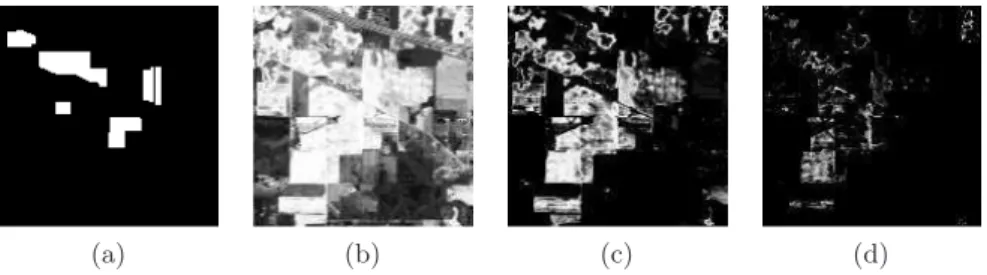
Figure 2. Influence of parameter σM P M on the computation of MPM using Euclidean distance, π M
k (x), for spectral class
2 of “Indian Pines”: (a) ground truth of the class; (b) σM P M = 1, (c) σM P M= 0.1, (d) σM P M = 0.01.
3. MODELLING MEMBERSHIP PROBABILITY MAP (MPM) OF SPECTRAL
CLASSES
Let us suppose that the spectral space of image fλ(x) is composed of K spectral classes: {C1, C2, · · · , CK}.
In addition, using a training set, each spectral class Ck is represented by a set of nk discrete spectra, i.e.,
Ck = {s1,k, s2,k, · · · , snk,k}, such that si,k∈ T
L.
Using a standard assumption on hyperspectral imaging, like it is considered for instance in target detection,8, 9
let us suppose that the points of each spectral classes follow a normal distribution in the space TL⊂ RL, i.e.,
Ck ≡ N (µk, Σk) where µk is the mean spectrum and Σk the covariance matrix of class Ck. Therefore, using
Bayesian terminology, the Gaussian conditional density per class is given by
Pr (si| Ck) = 1 (2π)L2|Σ k| L 2 e−12(si−µk) TΣ−1 k (si−µk)
According to the Bayes Decision Rule, the maximum a posteriori discriminant function becomes
gk(si) = Pr (Ck | si) = Pr (si| Ck) Pr (Ck) Pr (si) = 1 (2π)L2|Σ k| L 2 e−12(si−µk)TΣ−1k (si−µk)Pr (Ck) Pr (si)
and now, eliminating constant terms and taking natural logs (the logarithm is monotonically increasing), the classical quadratic discriminant function is obtained
gk(si) = − 1 2 h (si− µk)TΣ−1k (si− µk) i −1 2log (|Σk|) + log (Pr (Ck)) .
For convenience we assume also equiprobable priors so we can drop the term log (Pr (Ck)) (if the relative “size”
of each class in the image is known, the value of this term can be consequently calculated); it is also current to assume that |Σn| = |Σm| for any pair of classes n and m. Under these assumptions, the classical Mahalanobis
distance classifier is obtained
gk(si) = − 1 2 h (si− µk)TΣ−1(si− µk) i .
Another example of “metric” used widely in hyperspectral data processing for classification, detection, iden-tification, etc. is the Spectral Angle Mapper (SAM) algorithm.19 More precisely, the SAM calculates the angle between any pixel vector and a reference spectrum. It is well known that the angle (closely related also to the notion of correlation coefficient), as a normalized inner product, is an intensity independent measure: this is important for instance is the reference spectrum, as an average of representative spectra µk of class Ck, is
obtained from an image or database different from the current image. Hence, the SAM classifier is given by
hk(si) = −SAM (si, µk) = − arccos µ hsi, µki ksik · kµkk ¶ ,
where h·, ·i is the scalar product of two vectors and k · k is the norm of the vector.
(a1) (a2) (a3) (a4)
(b1) (b2) (b3) (b4)
(c1) (c2) (c3) (c4)
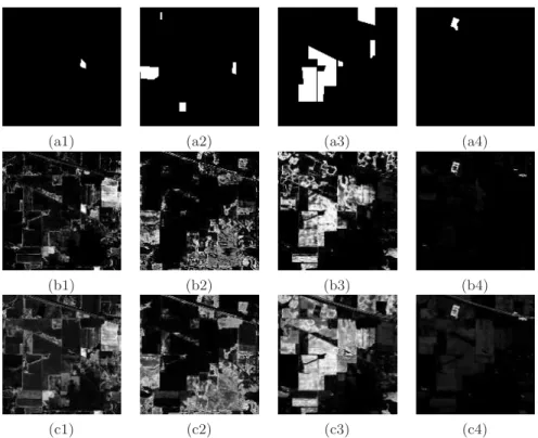
Figure 3. Comparison of MPM using Euclidean distance vs. Spectral Angle Mapper, for four spectral classes of “Indian Pines” (first column corresponds to class 1, second to class 5, third to class 11 and fourth to class 16): (a) ground truth of the class; (b) πM
k (x) with σM P M = 0.1; (c) πAk(x) with σM P M= 0.05.
Let us come back to our objective of probabilistic segmentation. Being inspired by these classical hyperspectral classifiers, we can now calculate for each class a scalar image πM
k (x) : E → R+, that we name membership
probability map (MPM) of the class Ck, which is defined by
πM k (x) = exp µ −1 2[(fλ(x)−µk)TΣ−1k (fλ(x)−µk)] σM P M ¶ P y∈Eexp µ −1 2[(fλ(y)−µk) TΣ−1 k (fλ(y)−µk)] σM P M ¶ .
This probability density function is proportional to a Gaussian-kernel version of the Mahalanobis distance com-puted for each pixel of the image. A high value of πk(x) implies that the image value spectrum fλ(x) has a high
probability to belongs to the class Ck.
If the number of spectral samples available for each class Ckis small (with respect to the spectral dimension),
the computation of the inverse of covariance matrix Σ−1k makes no sense and it may introduce important errors in the distance. A first approximation consist in considering only the band variances (i.e., Σk is a diagonal matrix).
But, in the experiments of this paper we use only 10 spectral samples as training set for each spectral class and consequently the most appropriate is to consider that Σk is the identity matrix: in summary, πMk (x) is based
on the Euclidean distance. The parameter σM P M allows to introduce a scaling regularization of the distance
values. In Fig. 2 is depicted an example, for spectral class 2 of “Indian Pines”, which illustrates the influence of parameter σM P M on the computation of MPM using Euclidean distance, πkM(x). The results are similar for
other classes, and empirically we found that σM P M = 0.1 produces a good trade-off. We can also notice that
this simple metric is not very specific for similar spectral classes: in the current example, several spectral regions of “corn vegetation” produces close values of πM
k (x).
Similarly, we can also calculate a MPM of the class Ck using the SAM, i.e.,
πA k(x) = exp³−SAM (fλ(x),µk) σM P M ´ P y∈Eexp ³ −SAM (fλ(x),µk) σM P M ´ .
A comparison of MPM using Euclidean distance vs. SAM, for four spectral classes of “Indian Pines”, is given in Fig. 3. On the basis of these examples, we conclude that for our purpose both approaches πM
k (x) and πAk(x)
lead to quite similar results and hence, for the experiments of this paper we will consider only πM
k (x), denoted
from now on by πk(x).
4. REGIONALIZED RANDOM GERMS SIMULATIONS FROM THE MPMS
We consider in this section the theoretical distribution which follows the regionalized random points as well as the algorithm used to simulate a realization of N random germs associated to each MPM.
4.1 Regionalized Poisson points
A rather natural way to introduce uniform random germs is to generate realizations of a Poisson point process with a constant intensity θ, namely average number of points per unit area. It is well known that the random number of points N (D) falling in a domain D, which is considered a bounded Borel set, with area |D|, follows a Poisson distribution with parameter θ|D|, i.e., . Pr{N (D) = n} = e−θ|D| (−θ|D|)n
n! . In addition, conditionally
to the fact that N (D) = n, the n points are independently and uniformly distributed over D, and the average number of points in D is θ|D| (i.e., the mean and variance of a Poisson distribution is its parameter).
More generally, we can suppose that the density θ is not constant; but considered as measurable function, defined in Rd, with positive values. For simplicity, let us write
θ(D) = Z
θ(x)dx
It is also known6, 7 that the number of points falling in a borel set B according to a regionalized density function
θ follows a Poisson distribution of parameter θ(D), i.e.,
Pr{N (D) = n} = e−θ(D)(−θ(D))
n
n! .
In such a case, if N (D) = n, the n are independently distributed over D with the probability density function b
4.2 Algorithm for simulation of germs for each spectral class
We have proposed above that each spectral class Ck of the hyperspectral image is modelled according to a MPM
πk(x); we notice that in this case the domain D corresponds to the discrete support space of the image. In
what follows, we are interested in generating a non-uniform distribution of germs, with a regionalized probability density function associated to class k such that bθ(x) ≡ πk(x).
In practice, in order to simulate a realization of N independent random germs distributed over the image with the pdf πk(x) we propose to use an inverse transform sampling method. More precisely, the algorithm to
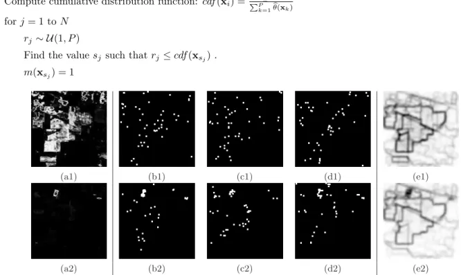
generate N randoms germs in an image m(x) according to density bθ(x) is as follows: 1. Initialization: m(xi) = 0 ∀xi∈ E; P = Card(E)
2. Compute cumulative distribution function: cdf (xi) = P k≤iθ(xb k) PP k=1bθ(xk) 3. for j = 1 to N 4. rj ∼ U(1, P )
5. Find the value sj such that rj ≤ cdf (xsj) .
6. m(xsj) = 1
(a1) (b1) (c1) (d1) (e1)
(a2) (b2) (c2) (d2) (e2)
Figure 4. MonteCarlo estimation of pdf of contours using SW for two spectral classes of “Indian Pines” (first row cor-responds to class 2 and second row to class 16): (a) MPM of the class πk(x); (b), (c) and (d) three realizations of 50
regionalized random points mrkπk
i (x) (the points have been dilated for a better visualization); (e) semi-supervised pdf of
contours pdfCk
(x) obtained from 50 realizations (in negative, the dark values correspond to high probabilities).
5. SEMI-SUPERVISED PROBABILITY DENSITY OF CONTOURS USING
STOCHASTIC WATERSHED
We have now all the ingredients for the semi-supervised SW. We start by considering that a MPM image is constructed for each spectral class of the hyperspectral image, i.e., {fλ(x), Ck} 7→ πk(x). As mentioned above,
πk(x) is obtained in all the experiments using the Euclidean distance, where the mean spectrum of the class
is computed from only 10 random training spectra of the class. Then, the MPM of each class is used as a regionalized density function to generate M realisations of N random points, i.e., πk(x) 7→ {mrkiπk(x)}Mi=1.
These images of random markers are employed to calculate the M realisations of watershed lines needed in the MonteCarlo procedure for estimation of the probability density of contours of spectral band λj with respect to
the class Ck, i.e.,
pdfCk λj (x) = 1 M M X i=1 W S(̺(fλj), mrk πk i )(x) ∗ K(x; σspatial).
Finally, as in the standard case, the pdf of the hyperspectral image w.r.t. the class Ck is obtained as the
kernelized sum of the marginal pdf’s of the spectral bands, i.e.,
{fλ(x), Ck} 7→ pdfCk(x) = 1 L L X j=1 pdfCk λj (x) ∗ K(λ; σspectral).
Examples of this MonteCarlo estimation of pdf of contours using SW, for two spectral classes of “Indian Pines”, are provided in Fig. 4; in particular, 3 realizations of 50 regionalized random points for each MPM are depicted. The pdf’s are estimated with 50 realizations of SW. We can observe that the contours of high probability from the pdf of each class correspond mainly to regions of the image associated to the spectral class according, of course, to the spectral discrimination specificity provided by the MPM. The class 16 (“Stone-steel towers”) of “Indian Pines” is a quite particular case which will be discussed in next section.
Once the pdf of the K classes has been computed, it is obvious that we can define a global pdf of the hyperspectral image as an average of the pdf of the different classes, i.e.,
pdfC(x) = 1 K K X k=1 pdfCk(x).
We must remark the this regionalized multi-class pdfC(x) is different from that obtained using uniform points
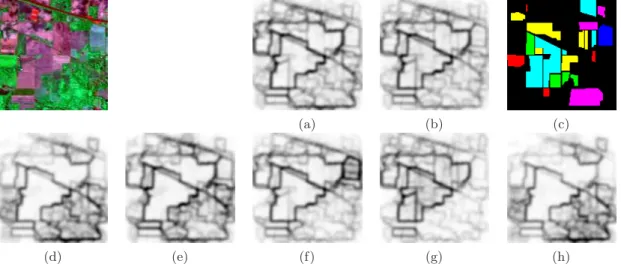
pdf (x), as discussed in Section 2. A comparison of both global pdf’s with respect to those of various spectral classes of “Indian Pines” are given in Fig. 5. From the examples we can state that, using the semi-supervised MonteCarlo framework of stochastic watershed, the image zones associated to the particular spectral class, which drove the simulation procedure, are enhanced with respect to the other zones. That involves that the contours of higher probability correspond to zones associated to the particular spectral class. However, as we can observe from the examples, these zones are not segmented as a single “region”; on the contrary, they are “segmented” in their various structural regions. Or in other words, zones which appear as a single connected component in the spectral ground truth are segmented in various spatial connected components.
(a) (b) (c)
(d) (e) (f) (g) (h)
Figure 5. MonteCarlo estimation of pdf’s of contours using SW for “Indian Pines”: (a) uniform unsupervised pdf of contours pdf (x); (b) semi-supervised multi-class pdf of contours pdfC
(x); (c) ground truth of some classes (in Yellow class 2 “Corn-notill”, in Red class 5 “grass/pasture”, in Green class 6 “grass/trees”, in Blue class 8 “hay-windrowed”, in Cyan class 11 “soybeans-min”, in Magenta class 14 “woods”). (d) semi-supervised pdf of contours of class 5 pdfC5
(x), (e) semi-supervised pdf of contours of class 6 pdfC6
(x), (f) semi-supervised pdf of contours of class 8 pdfC8
(x), (g) semi-supervised pdf of contours of class 11 pdfC11
(x), (h) semi-supervised pdf of contours of class 14 pdfC14
(a1) (a2) (a3) (a4) (a5)
(b1) (b2) (b3) (b4) (b5)
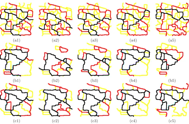
(c1) (c2) (c3) (c4) (c5)
Figure 6. Hierarchical segmentation of semi-supervised pdf’s of contours for “Indian Pines” (first column corresponds to multi-class pdfC
(x), second column to spectral class 5 pdfC5
(x), third column to spectral class 6 pdfC6
(x), fourth column to spectral class 8 pdfC8
(x) and fifth column to spectral class 11 pdfC11
(x)): (a) three levels of waterfalls algorithm (first in yellow, second in red and third in black); (b) three levels of dynamics-based segmentation in 5 regions (in yellow), 10 regions (in red) and 20 regions (in black); (c) three levels of volumic-based segmentation in 5 regions (in yellow), 10 regions (in red) and 20 regions (in black). The corresponding pdf’s are given in Fig. 5.
(a) (b) (c) (d)
Figure 7. Example of target region detection from semi-supervised pdf: (a) Initial image is the complemented pdf t0(x) =
−pdfC16
(x), (b) close-holes operator t1(x) = Cl-Holes(t0(x)), (c) negative of residue t2(x) = −|t0(x) − t1(x)|, (d) closing
t3(x) = ϕB(t2(x)) where B is a disk of 8 pixels.
6. PDFS POST-PROCESSING AND HIERARCHICAL SEGMENTATION
The pdfCk(x) could be directly thresholded in order to obtain the most prominent contours, however the results
are only pieces of contours (not enclosing regions). In addition, we have studied the histograms for several examples and there is not an optimal threshold to separate the classes of contours.
Let us start here by considering again the example of the pdf of class 16. The ground truth corresponds to a well defined spectral region which involves also a well defined spatial region of high probability in the pdf. Such a case, which can be considered as a problem target region detection, may be solved using standard morphological operators.14 In particular, the simple algorithm given in Fig. 7, based on classical operators like the close-holes
or closing using a disk as structuring element, illustrates how a region of a particular size/shape and a minimal value of probability detection can be extracted.
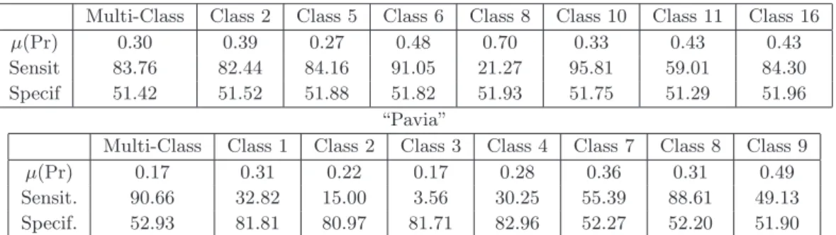
“Indian Pines”
Multi-Class Class 2 Class 5 Class 6 Class 8 Class 10 Class 11 Class 16 µ(Pr) 0.30 0.39 0.27 0.48 0.70 0.33 0.43 0.43 Sensit 83.76 82.44 84.16 91.05 21.27 95.81 59.01 84.30 Specif 51.42 51.52 51.88 51.82 51.93 51.75 51.29 51.96
“Pavia”
Multi-Class Class 1 Class 2 Class 3 Class 4 Class 7 Class 8 Class 9 µ(Pr) 0.17 0.31 0.22 0.17 0.28 0.36 0.31 0.49 Sensit. 90.66 32.82 15.00 3.56 30.25 55.39 88.61 49.13 Specif. 52.93 81.81 80.97 81.71 82.96 52.27 52.20 51.90
Table 1. Quantitative assessment of segmentation results for “Indian Pines” (segmentation of pdf’s in 100 dynamics-based regions) and “Pavia” (segmentation of pdf’s in 20 dynamics-based regions).
More generally, an alternative technique to segment automatically the pdf in significant closed regions is to apply a morphological hierarchical algorithm. Several watershed-based hierarchical approaches allow addressing imaging problems where the markers cannot be easily defined. Mainly, two hierarchical techniques can be distinguished:
i) Non-parametric waterfalls algorithm;4
ii) Hierarchies based on extinction values, which allows to select the minima used in the watershed according to morphological criteria (dynamics, surface area and volume).10, 17
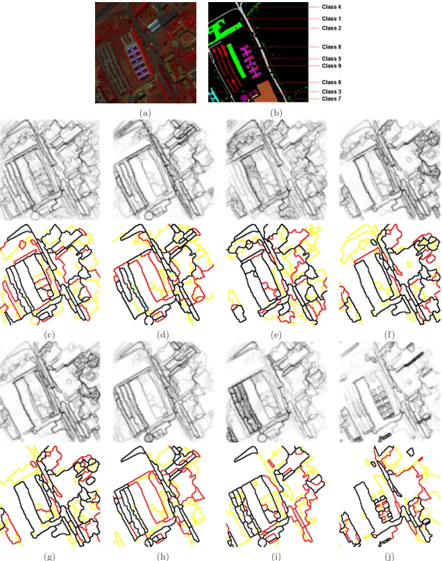
These methods of hierarchical segmentation have been used to segment the semi-supervised pdf’s of contours of “Indian Pines”. In Fig. 6 is given a systematic comparison for the pdf’s of four spectral classes together with the multi-class pdf. More precisely, it is shown the three first levels of waterfalls algorithm (first in yellow, second in red and third in black); three levels of dynamics-based segmentation in 5 regions (in yellow), 10 regions (in red) and 20 regions (in black) and three levels of volumic-based segmentation in 5 regions (in yellow), 10 regions (in red) and 20 regions (in black). In the three cases the obtained segmentations are coherent with the expected results according to the semi-supervised pdf’s. We observe also that the hierarchical segmentation for the multi-class pdf gives the most important image regions independently of the spectral behaviour. It seems in any case that, for the purpose of class-driven segmentation, the hierarchies based on the dynamics are particularly interesting. Indeed, the same algorithms of regionalized stochastic watershed have been also applied to the image “Pavia”. In Fig. 8 are depicted the results for a crop of the image. The comparison includes the multi-class pdf and seven of the semi-supervised spectral pdf’s (the image has nine spectral classes) as well as their hierarchical segmentations using dynamics criterion in 25 regions (in yellow), 50 regions (in red) and 100 regions (in black). We observe the visual quality of the semi-supervised pdf’s and subsequent segmentations are relatively good, taking into account the structural complexity of the image.
By selecting a particular level of the dynamics-based hierarchy, which involves selecting a priori the number of regions, a more quantitative assessment of the segmentation results can be achieved. More precisely, using the ground truth segmentations of each class, we have compared quantitatively the performances by computing three parameters: i) the average probability of pdfCkon the ground truth contours, denoted by µ(Pr), ii) the sensitivity
percentage Sensit = 100T P/(T P + F N ), iii) the specificity percentage Specif = 100T N/(T N + F P ); (where T P , T N , F P , F N are defined in terms of pixels of the contours). The values for a both images are given in the Table 1. As we can observe, the quantitative results for “Indian Pines” are better than for “Pavia”: the reference contours of spectral regions of “Pavia” are often associated to narrow regions and their correspondence with the obtained contours is not always perfectly located. In addition, we notice again that these results correspond to a segmentation in a fixed number of regions. More evolved techniques for an accuracy assessment of the segmentation, as recently proposed in,13 can be used for a most systematic evaluation of results and in order to
optimize the parameters for particular applications.
7. CONCLUSION AND PERSPECTIVES
We have introduced in this paper a novel probabilistic framework for semi-supervised image segmentation in high spatial resolution hyperspectral images using stochastic watershed, and without using classification
tech-niques. The required information is a training set of representative spectra of each spectral class and produces a probability density function of contours for each class, plus a global multi-class pdf.
We can conclude the empirical study by saying that our approach of stochastic segmentation performs rela-tively well, except for image regions with very irregular contours or regions associated to spectral classes which are not well sampled during the regionalized simulation procedure. In fact, the main limitation of our approach is given by the simplicity of modelling the membership probability map, which involves an unspecific regionalized simulation of germs. If this step is improved, using advanced machine learning techniques the quality of the final pdf, and subsequent segmentation, would be also improved. In addition, work remains to be done in the integra-tion of the semi-supervised spatial informaintegra-tion, associated to the probability of a pixel to belong to a contour of a particular spectral class, with the spectral information of the pixel used for classification. A promising direction is to use graph-based semi-supervised image segmentation techniques integrating spatial-spectral kernels.18
Acknowledgment. The authors would like to thank the IAPR-TC7 for providing the data, and Prof. P. Gamba and Prof. F. Dell’Acqua of the University of Pavia, Italy, for providing reference data.
REFERENCES
[1] J. Angulo, D. Jeulin. Stochastic watershed segmentation. In Proc. Int. Symp. Mathematical Morphology
ISMM’07, Rio, Brazil, INPE, Eds. Banon, G. et al., 265–276, 2007.
[2] J. Angulo, S. Velasco-Forero, J. Chanussot. Multiscale stochastic watershed for unsupervised hyperspectral image segmentation. In Proc. of IEEE IGARSS’2009, Vol. III, 93–96, Cape Town, South Africa, July 2009. [3] S. Beucher, F. Meyer. The Morphological Approach to Segmentation: The Watershed Transformation. In
Mathematical Morphology in Image Processing, Marcel Dekker, Eds. E. Dougherty, 1992, 433–481, 1992.
[4] S. Beucher. Watershed, hierarchical segmentation and waterfall algorithm. In Mathematical Morphology and
its Applications to Image and Signal Processing, Proc. ISMM’94 Kluwer, 69–76, 1994.
[5] O. Chapelle, B. Sch¨olkopf and A. Zien. Semi-Supervised Learning. MIT Press, Cambridge, MA, 2006. [6] C. Lantu´ejoul. Geostatistical Simulation: Models and Algorithms, Springer-Verlag, Heidelberg, Berlin, 2002. [7] G. Matheron. Random sets and integral geometry, Wiley, New York, 1975.
[8] D.G. Manolakis, V.K. Ingle, S.M. Kogon. Statistical and Adpative Signal Processing: Spectral Estimation,
Signal Modelling, Adaptive Filtering and Array Processing, McGraw-Hill, Boston, 2000.
[9] D.G. Manolakis, C. Siracusa, G. Shaw. Hyperspectral Subpixel Target Detection Using the Linear Mixing Model. IEEE Trans. on Geoscience and Remote Sensing, Vol. 39, No. 7, 2001.
[10] F. Meyer. An Overview of Morphological Segmentation. International Journal of Pattern Recognition and
Artificial Intelligence Vol. 15, No. 7, 1089-1118, 2001.
[11] G. Noyel, J. Angulo, D. Jeulin. Random Germs and Stochastic Watershed for Unsupervised Multispectral Image Segmentation. In Proc. KES 2007/ WIRN 2007, Part III, LNAI 4694, Springer, 17–24, 2007. [12] G. Noyel, J. Angulo, D. Jeulin. Classification-driven stochastic watershed. Application to multispectral
segmentation. In Proc. of the IS&T’s Fourth European Conference on Color on Graphics, Imaging and
Vision (CGIV’2008), Terrasa-Barcelona, Spain, 471–476, 2008.
[13] C. Persello, L. Bruzzone. A Novel Protocol for Accuracy Assessment in Classification of Very High Resolution Images. IEEE Trans. on Geoscience and Remote Sensing, Vol. 48, No. 3, 1232–1244, 2010.
[14] P. Soille. Morphological image analysis, Springer-Verlag, Berlin Heidelberg, 1999.
[15] Y. Tarabalka, J. Chanussot, J.-A. Benediktsson, J. Angulo, M. Fauvel. Segmentation and classification of hyperspectral data using watershed. In Proc. of IEEE IGARSS’08, Boston-Massachusetts, USA, July 2008. [16] Y. Tarabalka, J. Chanussot, J.-A. Benediktsson. Segmentation and classification of hyperspectral images
using watershed transformation. Pattern Recognition, 2010.
[17] C. Vachier, F. Meyer. Extinction value: a new measurement of persistence. IEEE Workshop on Nonlinear
Signal and Image Processing, pp. 254–257, 1995.
[18] S. Velasco-Forero, V. Manian. Improving Hyperspectral Image Classification Using Spatial Preprocessing.
IEEE Geoscience and Remote Sensing Letters, 6(2): 297–301, 2009.
[19] R.H. Yuhas, A.F.H. Goetz, J.W. Boardman. Discrimination among semiarid landscape endmembers using the spectral angle mapper (SAM) algorithm. In Summaries of the Third Annual JPL Airborne Geoscience
(a) (b)
(c) (d) (e) (f)
(g) (h) (i) (j)
Figure 8. Semi-supervised spectral-driven pdf’s of contours for a part of the hyperspectral imge “Pavia” and their hier-archical segmentations using dynamics criterion in 25 regions (in yellow), 50 regions (in red) and 100 regions (in black): (a) original image from significant spectral bands, (b) ground truth for the nine spectral classes, (c) multi-class pdfC
(x), (d) spectral class 1 pdfC1
(x), (e) spectral class 2 pdfC2
(x), (f) spectral class 3 pdfC3
(x), (g) spectral class 4 pdfC4
(x), (h) spectral class 7 pdfC7
(x), (i) spectral class 8 pdfC8
(x), (j) spectral class 9 pdfC9