Multi-player games in the era of machine learning

(1)

Université de Montréal

Multi-player Games in the Era of Machine

Learning

par

Gauthier Gidel

Département d’informatique et de recherche opérationnelle Faculté des arts et des sciences

Thèse présentée à la Faculté des arts et des sciences en vue de l’obtention du grade de Philosophiæ Doctor (Ph.D.)

en informatique

July, 2020

c

(2)

Université de Montréal Faculté des arts et des sciences

Cette thèse intitulée:

Multi-player Games in the Era of Machine

Learning

présentée par:

Gauthier Gidel

a été évaluée par un jury composé des personnes suivantes: Ioannis Mitliagkas, président-rapporteur Simon Lacoste-Julien, directeur de recherche Yoshua Bengio, membre du jury Constantinos Daskalakis, examinateur externe

(3)

À toi qui lis ces lignes, et à la beauté qui te guide. To you who read these lines, and to the beauty guiding you.

(4)

Résumé

Parmi tous les jeux de société joués par les humains au cours de l’histoire, le jeu de go était considéré comme l’un des plus difficiles à maîtriser par un programme informatique [Van Den Herik et al.,2002]; Jusqu’à ce que ce ne soit plus le cas [Silver et al.,2016]. Cette percée révolutionnaire [Müller,2002,Van Den Herik et al.,2002] fût le fruit d’une combinaison sophistiquée de Recherche arborescente Monte-Carlo et de techniques d’apprentissage automatique pour évaluer les positions du jeu, mettant en lumière le grand potentiel de l’apprentissage automatique pour résoudre des jeux.

L’apprentissage antagoniste, un cas particulier de l’optimisation multiobjective, est un outil de plus en plus utile dans l’apprentissage automatique. Par exemple, les jeux à deux joueurs et à somme nulle sont importants dans le domain des réseaux génératifs antagonistes [Goodfellow et al., 2014] et pour maîtriser des jeux comme le Go ou le Poker en s’entraînant contre lui-même [Silver et al., 2017, Brown and Sandholm, 2017]. Un résultat classique de la théorie des jeux indique que les jeux convexes-concaves ont toujours un équilibre [Neumann, 1928]. Étonnamment, les praticiens en apprentissage automatique entrainent avec succès une seule paire de réseaux de neurones dont l’objectif est un problème de minimax non convexe et non concave alors que pour une telle fonction de gain, l’existence d’un équilibre de Nash n’est pas garantie en général. Ce travail est une tentative d’établir une solide base théorique pour l’apprentissage dans les jeux.

La première contribution explore le théorème minimax pour une classe partic-ulière de jeux nonconvexes-nonconcaves qui englobe les réseaux génératifs antago-nistes. Cette classe correspond à un ensemble de jeux à deux joueurs et a somme nulle joués avec des réseaux de neurones.

Les deuxième et troisième contributions étudient l’optimisation des problèmes minimax, et plus généralement, les inégalités variationnelles dans le cadre de l’apprentissage automatique. Bien que la méthode standard de descente de gradient ne parvienne pas à converger vers l’équilibre de Nash de jeux convexes-concaves sim-ples, il existe des moyens simples d’utiliser des gradients pour obtenir des méthodes qui convergent. Nous étudierons plusieurs techniques telles que l’extrapolation, la moyenne et la quantité de mouvement à paramètre négatif.

La quatrième contribution fournit une étude empirique du comportement pra-tique des réseaux génératifs antagonistes. Dans les deuxième et troisième contribu-tions, nous diagnostiquons que la méthode du gradient échoue lorsque le champ de vecteur du jeu est fortement rotatif. Cependant, une telle situation peut décrire un

(5)

pire des cas qui ne se produit pas dans la pratique. Nous fournissons de nouveaux outils de visualisation afin d’évaluer si nous pouvons détecter des rotations dans comportement pratique des réseaux génératifs antagonistes.

(6)

Abstract

Among all the historical board games played by humans, the game of go was con-sidered one of the most difficult to master by a computer program [Van Den Herik et al., 2002]; Until it was not [Silver et al., 2016]. This odds-breaking break-through [Müller, 2002, Van Den Herik et al., 2002] came from a sophisticated combination of Monte Carlo tree search and machine learning techniques to evalu-ate positions, shedding light upon the high potential of machine learning to solve games.

Adversarial training, a special case of multiobjective optimization, is an increas-ingly useful tool in machine learning. For example, two-player zero-sum games are important for generative modeling (GANs) [Goodfellow et al.,2014] and mastering games like Go or Poker via self-play [Silver et al., 2017, Brown and Sandholm,

2017]. A classic result in Game Theory states that convex-concave games always have an equilibrium [Neumann, 1928]. Surprisingly, machine learning practitioners successfully train a single pair of neural networks whose objective is a nonconvex-nonconcave minimax problem while for such a payoff function, the existence of a Nash equilibrium is not guaranteed in general. This work is an attempt to put learning in games on a firm theoretical foundation.

The first contribution explores minimax theorems for a particular class of nonconvex-nonconcave games that encompasses generative adversarial networks. The proposed result is an approximate minimax theorem for two-player zero-sum games played with neural networks, including WGAN, StarCrat II, and Blotto game. Our findings rely on the fact that despite being nonconcave-nonconvex with respect to the neural networks parameters, the payoff of these games are concave-convex with respect to the actual functions (or distributions) parametrized by these neural networks.

The second and third contributions study the optimization of minimax prob-lems, and more generally, variational inequalities in the context of machine learn-ing. While the standard gradient descent-ascent method fails to converge to the Nash equilibrium of simple convex-concave games, there exist ways to use gradi-ents to obtain methods that converge. We investigate several techniques such as extrapolation, averaging and negative momentum. We explore these technique ex-perimentally by proposing a state-of-the-art (at the time of publication) optimizer for GANs called ExtraAdam. We also prove new convergence results for Extrapo-lation from the past, originally proposed by Popov [1980], as well as for gradient method with negative momentum.

(7)

The fourth contribution provides an empirical study of the practical landscape of GANs. In the second and third contributions, we diagnose that the gradient method breaks when the game’s vector field is highly rotational. However, such a situation may describe a worst-case that does not occur in practice. We provide new visualization tools in order to exhibit rotations in practical GAN landscapes. In this contribution, we show empirically that the training of GANs exhibits significant rotations around Local Stable Stationary Points (LSSP), and we provide empirical evidence that GAN training converges to a stable stationary point which, is a saddle point for the generator loss, not a minimum, while still achieving excellent performance.

(8)

Keywords—Mots-clés

machine learning, game theory, adversarial training, minimax, Nash equilib-rium, optimization, multi-player games, variational inequality, generative adver-sarial networks, extragradient, generative modeling, landscape visualization, mo-mentum.

apprentissage statistique, théorie des jeux, apprentissage antagoniste, mini-max, equilibre de Nash, optimisation, jeux a somme nulle, inégalités variationelles, réseaux génératifs antagonistes, extragradient, model génératifs, visualisation de champ de vecteurs, méthode du moment.

(9)

List of Tables

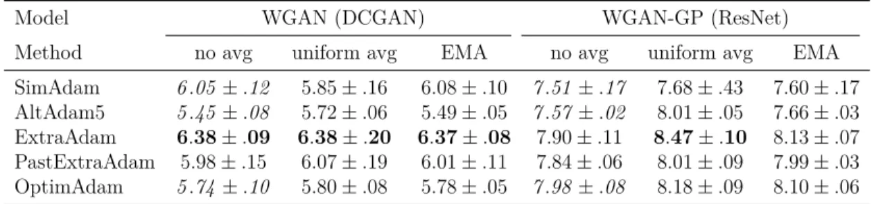
6.1 Best inception scores (averaged over 5 runs) achieved on CIFAR10 for every considered Adam variant. OptimAdam is the related Op-timistic Adam [Daskalakis et al., 2018] algorithm. EMA denotes exponential moving average (with β = 0.9999, see Eq. 3.2). We see that the techniques of extrapolation and averaging consistently enable improvements over the baselines (in italic). . . 57

10.1 Summary of the implications between Differentiable Nash Equilibrium (DNE) and a locally stable stationnary point (LSSP): in general, being a DNE is neither necessary or sufficient for being a LSSP. . . 82 B.1 DCGAN architecture used for our CIFAR-10 experiments. When

using the gradient penalty (WGAN-GP), we remove the Batch Nor-malization layers in the discriminator.. . . 150

B.2 Best inception scores (averaged over 5 runs) achieved on CIFAR10 for every considered Adam variant. We see that the techniques of extrapolation and averaging consistently enable improvements over the baselines (in italic). . . 151

B.3 ResNet architecture used for our CIFAR-10 experiments. When us-ing the gradient penalty (WGAN-GP), we remove the Batch Nor-malization layers in the discriminator.. . . 152

B.4 Best FID scores (averaged over 5 runs) achieved on CIFAR10 for ev-ery considered Adam variant. OptimAdam is the related Optimistic Adam [Daskalakis et al., 2018] algorithm. We see that the tech-niques of extrapolation and EMA consistently enable improvements over the baselines (in italic). . . 152

(15)

List of Figures

4.1 Training of latent agents to play differentiable Blotto with K = 3. Right: The suboptimality corresponds to the payoff of the agent against a best response. We averaged our results over 40 random seeds. . . 37 6.1 Comparison of the basic gradient method (as well as Adam) with the

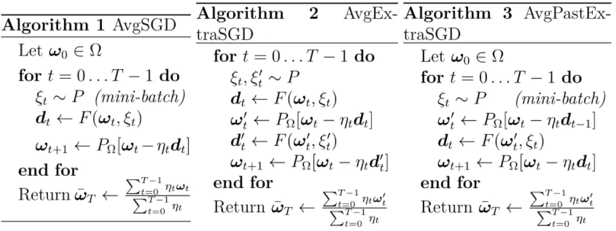
techniques presented in §3 on the optimization of (3.3). Only the algo-rithms advocated in this paper (Averaging, Extrapolation and Extrap-olation from the past) converge quickly to the solution. Each marker represents 20 iterations. We compare these algorithms on a non-convex objective in §7.1. . . 49 6.2 Three variants of SGD computing T updates, using the techniques

introduced in §3. . . 50

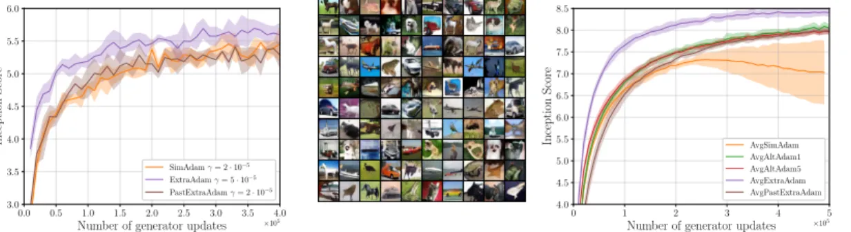
6.3 Performance of the considered stochastic optimization algorithms on the bilinear problem (7.1). Each method uses its respective optimal step-size found by grid-search. . . 55 6.4 Left: Mean and standard deviation of the inception score computed over

5 runs for each method on WGAN trained on CIFAR10. To keep the graph readable we show only SimAdam but AltAdam performs similarly.

Middle: Samples from a ResNet generator trained with the

WGAN-GP objective using AvgExtraAdam. Right: WGAN-GP trained on CIFAR10: mean and standard deviation of the inception score computed over 5 runs for each method using the best performing learning rates; all experiments were run on a NVIDIA Quadro GP100 GPU. We see that ExtraAdam converges faster than the Adam baselines. . . 58 8.1 Left: Decreasing trend in the value of momentum used for training

GANs across time. Right: Graphical intuition of the role of mo-mentum in two steps of simultaneous updates (tan) or alternated

updates (olive). Positive momentum (red) drives the iterates

out-wards whereas negative momentum (blue) pulls the iterates back

towards the center, but it is only strong enough for alternated up-dates. . . 62

8.2 Effect of gradient methods on an unconstrained bilinear example: minθmaxϕ θ>Aϕ.The quantity ∆t is the distance to the optimum

(16)

8.3 Eigenvalues λ_i of the Jacobian_∇v(φ∗, θ∗), their trajectories 1_{− ηλ}_i for growing step-sizes, and the optimal step-size. The unit circle is drawn in

black, and thereddashed circle has radius equal to the largest eigenvalue

µ_max, which is directly related to the convergence rate. Therefore, smaller red circles mean better convergence rates. Top: The red circle is limited by the tangent trajectory line 1_{− ηλ}₁, which means the best convergence rate is limited only by the eigenvalue which will pass furthest from the origin as η grows, i.e., λ_i = arg min_<(1/λ_i). Bottom: The red circle is cut (not tangent) by the trajectories at points 1_{− ηλ}₁ and 1_{− ηλ}₃. The

η is optimal because any increase in η will push the eigenvalue λ₁ out of the red circle, while any decrease in step-size will retract the eigenvalue

λ3 out of the red circle, which will lower the convergence rate in any case.

Figure inspired by Mescheder et al. [2017]. . . . 66

8.4 Transformation of the eigenvalues by the negative momentum method for a game introduced in (2.4) with d = p = 1, A = 1, α = 0.4, η = 1.55, β =_−0.25. Convergence circles for gradient method are inred, negative momentum

in green, and unit circle in black. Solid convergence circles are

optimized over all step-sizes, while dashed circles are at a given step-size

η. For a fixed η, original eigenvalues are inredand negative momentum eigenvalues are in blue. Their trajectories as η sweeps in [0, 2] are in light colors. Negative momentum helps as the new convergence circle (green) is smaller, due to shifting the original eigenvalues (red dots) towards the origin (right blue dots), while the eigenvalues due to state augmentation (left blue dots) have smaller magnitude and do not influence the convergence rate. Negative momentum allows faster convergence (green circle is inside the solid red circle) for a much broader range of step-sizes. . . 67 8.5 The effect of momentum in a simple min-max bilinear game where the

equilibrium is at (0, 0). (left-a) Simultaneous GD with no momentum

(left-b) Alternating GD with no momentum. (left-c) Alternating GD

with a momentum of +0.1. (left-d) Alternating GD with a momentum of_{−0.1. (right) A grid of experiments for alternating GD with different} values of momentum (β) and step-sizes (η): While any positive momen-tum leads to divergence, small enough value of negative momenmomen-tum allows for convergence with large step-sizes. The color in each cell indicates the normalized distance to the equilibrium after 500k iteration, such that 1.0 corresponds to the initial condition and values larger (smaller) than 1.0 correspond to divergence (convergence). . . 71

(17)

8.6 Comparison between negative and positive momentum on GANs with saturating loss on CIFAR-10 (left) and on Fashion MNIST (right) using a residual network. For each dataset, a grid of different values of momen-tum (β) and step-sizes (η) is provided which describes the discriminator’s settings while a constant momentum of 0.5 and step-size of 10−4 is used for the generator. Each cell in CIFAR-10 (or Fashion MNIST) grid con-tains a single configuration in which its color (or its content) indicates the inception score (or a single sample) of the model. For CIFAR-10 ex-periments, yellow is higher while blue is the lower inception score. Along each row, the best configuration is chosen and more samples from that configuration are presented on the right side of each grid. . . 73 10.1 Visualizations of Example 4. Left: projection of the game vector field on

the plane θ₂ = 1. Right: Generator loss. The descent direction is (1, ϕ) (in grey). As the generator follows this descent direction, the discrimina-tor changes the value of ϕ, making the saddle rotate, as indicated by the circular black arrow. . . 83 10.2 Above: game vector field (in grey) for different archetypal

behav-iors. The equilibrium of the game is at (0, 0). Black arrows corre-spond to the directions of the vector field at different linear inter-polations between two points: • and ?. Below: path-angle c(α) for different archetypal behaviors (right y-axis, in blue). The left y-axis in orange correspond to the norm of the gradients. Notice the "bump" in path-angle (close to α = 1), characteristic of rotational dynamics. . . 86

10.3 Path-angle for NSGAN (top row) and WGAN-GP (bottom row) trained on the different datasets, see Appendix D §3.3 for details on how the path-angle is computed. For MoG the ending point is a generator which has learned the distribution. For MNIST and CI-FAR10 we indicate the Inception score (IS) at the ending point of the interpolation. Notice the “bump" in path-angle (close to α = 1.0), characteristic of games rotational dynamics, and absent in the min-imization problem (d). Details on error bars in Appendix D §3.3. . 88

10.4 Eigenvalues of the Jacobian of the game for NSGAN (top row) and WGAN-GP (bottom row) trained on the different datasets. Large imaginary eigenvalues are characteristic of rotational behavior. Notice that NSGAN and WGAN-GP objectives lead to very different landscapes (see how the eigenvalues of WGAN-GP are shifted to the right of the imaginary axis). This could explain the difference in performance between NSGAN and WGAN-GP. . . 89

(18)

10.5 NSGAN. Top k-Eigenvalues of the Hessian of each player (in terms of magnitude) in descending order. Top Eigenvalues indicate that the Generator does not reach a local minimum but a saddle point (for CIFAR10 actually both the generator and discriminator are at saddle points). Thus the training algorithms converge to LSSPs which are not Nash equilibria. . . 90

10.6 WGAN-GP. Top k-Eigenvalues of the Hessian of each player (in terms of magnitude) in descending order. Top Eigenvalues indicate that the Generator does not reach a local minimum but a saddle point. Thus the training algorithms converge to LSSPs which are not Nash equilibria. . . 91

A.1 Difference between pointwise averaging of function and latent mix-ture of mapping. . . 116

B.1 Comparison of five algorithms (described in Section 3) on the non-convex GAN objective (7.1), using the optimal step-size for each method. Left: The gradient vector field and the dynamics of the different methods. Right:The distance to the optimum as a function of the number of iterations. . . 149

B.2 DCGAN architecture with WGAN-GP trained on CIFAR10: mean and standard deviation of the inception score computed over 5 runs for each method using the best performing learning rate plotted over number of generator updates (Left) and wall-clock time (Right); all experiments were run on a NVIDIA Quadro GP100 GPU. We see that ExtraAdam converges faster than the Adam baselines. . . 151

B.3 Inception score on CIFAR10 for WGAN-GP (DCGAN) over number of generator updates for different learning rates. We can see that AvgExtraAdam is less sensitive to the choice of learning rate. . . 153

B.4 Comparison of the samples quality on the WGAN-GP (DCGAN) experiment for different methods and learning rate η. . . . 154

B.5 Inception Score on CIFAR10 for WGAN over number of generator updates with and without averaging. We can see that averaging improve the inception score. . . 155

B.6 Inception score on CIFAR10 for WGAN-GP (DCGAN) over number of generator updates . . . 156

B.7 Comparison of the samples of a WGAN trained with the different methods with and without averaging. Although averaging improves the inception score, the samples seem more blurry . . . 157

(19)

B.8 The Fréchet Inception Distance (FID) from Heusel et al. [2017] com-puted using 50,000 samples, on the WGAN experiments. ReEx-traAdam refers to Alg. 5 introduced in §4. We can see that averag-ing performs worse than when comparaverag-ing with the Inception Score. We observed that the samples generated by using averaging are a little more blurry and that the FID is more sensitive to blurriness, thus providing an explanation for this observation.. . . 158

C.1 Contour plot of the maximum magnitude of the eigenvalues of the polynomial (x − 1)2_{(x − β)}2 _{+ η}2_x2 _{(left, simultaneous) and}

(x − 1)2_{(x − β)}2 _{+ η}2_x3 _{(right, alternated) for different values of}

the step-size η and the momentum β. Note that compared to (5.5) and (5.7) we used β1 = β2 = β and we defined η := √η1η2λ without

loss of generality. On the left, magnitudes are always larger than 1, and equal to 1 for β = −1. On the right, magnitudes are smaller than 1 for η

2 − 1 ≤ β ≤ 0 and greater than 1 elsewhere. . . . 161

C.2 The effect of negative momentum for a mixture of 8 Gaussian dis-tributions in a GAN setup. Real data and the results of using SGD with zero momentum on the Generator and using negative / zero / positive momentum (β) on the Discriminator are depicted. . . . . 162

C.3 Plot of the optimal value of momentum by for different α’s and con-dition numbers (log10κ). Blue/white/orange regions correspond to

negative/zero/positive values of the optimal momentum, respectively.164

D.1 The norm of gradient during training for the standard GAN objec-tive. We observe that while extra-gradient reaches low norm which indicates that it has converged, the gradient descent on the contrary doesn’t seem to converge.. . . 189

D.2 Path-angle and Eigenvalues computed on MNIST with Adam.. . . 189 D.3 Path-angle and Eigenvalues for NSGAN on CIFAR10 computed on

CI-FAR10 with Adam. We can see that the model has eigenvalues with negative real part, this means that we’ve actually reached an unstable point. . . 190

(20)

List of acronyms and

abbreviations

CCE coarse correlated equilibria e.g. exempli gratia [for instance] EG Extragradient Method ERM Empirical Risk Minimization i.e. ide est [that is]

GANs Generative Adversarial Networks LSSE Locally Stable Stationnary Point ML Machine Learning

NE Nash Equilibrium PPM Proximal-Point Method resp. respectively

SGD Stocastic Gradient Descent VIP Variational Inequality Problem

(21)

Acknowledgements

Aaron, Adam, Adrien, Ahmed, Alais, Amjad, Amy, Antoine, Ariane, Aude, Audrey, Alex, Alexandre, Alberto, Anna, Anne Marie, Annabel, Aristide, Arthur, Aymeric, Benoît (Beubeu), Bérénice, Camille, Catherine, Christophe, Claire, Clément (Clemsy), Danielle, Damien, David, Denise, Dzmitry, Élodie, Emma, Elise, Elyse, Eugene, Fabian, Florent, Florestan (Floflo), Francis, François, Félix, Fernand, Francesco, Gaëtan, Gabriel, Gabriella (Gaby), Garo, Geneviève (Geugeu), Georgios, Giancarlo, Grace, Guillaume, Gul, Guy (Gitou), Hélene, Hirosuke (Hiro), Hugo, Ian, Idriss, Ioannis, Issam, Jacques (Jak), Jaime, James, Jean Baptiste, Jeanne, Jérémy, Joey, Judith, Kawtar, Kyle, Laura, Laure, Léna, Léonie, Linda, Lucie, Loïc, Loucas, Marie-Auxille, Marion, Mark, Marta, Marie Christine, Maryse, Mastro, Mathieu, Maximilian, Max, Michel, Mickaël (Mika), Mohamad, Mohammad, Morgane, Myrto, Nazia, Niao, Nicolas, Olivier, Oscar, Pascal, Pierre, Quentin, Raphaël, Reyhane, Rémi, Rim, Robert, Romain, Salem, Sharan, Sébastian, Sébastien, Serge, Sandra, Samy, Sesh, Simon, Sophie, Tanis, Tanja, Tatjana, Tess, Theodor, Thomas, Tom, Tommy, Tony, Tristan, Tweety, Utku, Valentin, Veranika, Victor, Vincent, Yan, Yann (Yannou), Yana, Yoram, Yoshua, Ylva, Waïss, Wojtek, Zhor, Ziad.

Merci a toi que j’ai peut-être apprécié, respecté, aimé, idolatré ou detesté; avec qui j’ai parlé, échangé, fait de la recherche, souri, rêvé, ri, ou pleuré. Ma thèse fut un long voyage dont tu as fait partie. Nos chemin se sont croisé, et se recroiserons peut-être.

Thanks to you who I may have appreciated, respected, loved, idolized or hated; with whom I spoke, interacted, did research, smiled, dreamt, laughed, or cried. My thesis was a long journey you were part of. Our paths crossed and may cross again.

(22)

Notation

The set of real numbers . . . R The set of complex numbers . . . C

The real and imaginary part of z ∈ C . . . . . <(z) and =(z) Scalars are lower-case letters . . . λ

Vectors are lower-case bold letters . . . θ Matrices are upper-case bold letters. . . A Operators are upper-case letters . . . F The spectrum of a squared matrix A . . . Sp(A) The spectral radius of a squared matrix A . . . ρ(A)

The largest and the smallest singular values of A σmin(A) and σmax(A) The identity matrix of Rd×d . . . _I

d

(23)

1

Introduction

«On a pas les mêmes règles pourtant c’est le même jeu»

[We do not have the same rules yet it’s the same game]–Lomepal [2019]

What is the game mentioned by Lomepal [2019]? For some, it could be the game of life [Gardner,1970], while for others, it remains a mystery. However, what is certain is that we live in a world full of games. From the simplest ones, such as rock-paper-scissor, to the most challenging ones such as chess, go, or StarCraft II, games are so complex and interesting that there exist a professional league of players and dense theoretical literature for each of them [Simon and Chase, 1988,

Bozulich,1992, Vinyals et al.,2017].

That is why a long-standing goal in artificial intelligence [Samuel,1959,Tesauro,

1995, Schaeffer, 2000] has been to achieve superhuman performance—with a com-puter program—at such games of skills.

Among all the historical board games played by humans, the game of go was con-sidered one of the most difficult to master by a computer program [Van Den Herik et al., 2002]; Until it was not [Silver et al., 2016]. This odds-breaking break-through [Müller, 2002, Van Den Herik et al., 2002] came from a sophisticated combination of Monte Carlo tree search and machine learning techniques to evalu-ate positions, shedding light upon the high potential of machine learning to solve games.

Machine learning, the science of learning mathematical models from data, has expanded significantly in the last two decades. It has had a noticeable impact in diverse areas such as computer vision [Krizhevsky et al., 2012], speech recognition [Hinton et al., 2012], natural language processing [Sutskever et al.,

2014], computational biology [Libbrecht and Noble, 2015], and medicine [Esteva et al., 2017].

Interestingly, while regarding such different domains, these success stories have a common ground: they all correspond to the estimation of a prediction function based on empirical data [Vapnik,2006]. This learning paradigm, based on empirical risk minimization (ERM), is known as supervised learning. At a high level, esti-mating the correct dependence through ERM requires three main ingredients: 1) a sufficient amount of data, 2) a hypothesis class on the actual dependence function, 3) a sufficient amount of computing to find an approximate solution to the corre-sponding minimization problem. These three steps are subject to interdependent tradeoffs [Bottou and Bousquet, 2008]—for instance, for a given computational

(24)

budget, more data would improve our ability to generalize but would make the optimization procedure harder—are at the heart of the challenges of supervised learning.

The notable success of the applications of supervised learning mentioned above can be attributed to many factors. Among them, one can arguably say that the building of high-quality datasets [Russakovsky et al., 2015], the improved access to computational resources, and the design of scalable training methods for large models [LeCun et al., 1998] played a significant role.

However, yet powerful, supervised learning is a restrictive setting where a single learner is in a fixed environment, i.e., it has access to a large number of input-output pairs at training time that come from an independent and identically distributed process. This assumption does not consider that some other agents, i.e., computer programs or humans, maybe part of the environment and thus impact the task.

Real-world games such as Go, poker, or chess are composed of multiple players, thus not fitting into the i.i.d. ERM framework that is composed of a single learner in a fixed environment. From the players’ viewpoint, the environment that conditions the way they should play depends on their opponent and thus is not fixed. From a machine learning perspective, the task in those games is to learn how to play to beat any opponent.

Recently, machine learning techniques have led to significant progress on in-creasingly complex domains such as classical board games (e.g., chess [Silver et al.,

2018] or go [Silver et al., 2017]), card games (e.g., poker [Brown and Sandholm,

2017, 2019] or Hanabi [Foerster et al., 2019]), as well as video games (e.g., Star-Craft II [Vinyals et al., 2019] or Dota 2 [Berner et al., 2019]). However, chess, go, and more generally, all the zero-sum games of skills mentioned in this introduction are just “a Drosophilia of reasoning” [Kasparov, 2018]. We are just scratching the surface, the combination of multi-player games and machine learning can offer.

1 Multiplayer games and Machine Learning

Adversarial formulations, or more generally multi-player games, are frameworks that aim at casting tasks into which several agents (a.k.a players) compete (or col-laborate) to solve a problem. At a high level, each agent is given a set of parameters and a loss that they try to minimize. The key difference between standard super-vised learning and multi-player games is that each agent’s loss depends on all the players’ parameters, thus entangling the minimization problem of each player.

Such frameworks include real-world games such as Backgammon, poker, or Starcraft II, but also market mechanisms [Nisan et al., 2007], auctions [Vickrey,

1961], as well as games specifically designed for a machine learning purpose such as Generative Adversarial Networks (GANs) [Goodfellow et al., 2014] that enabled a

(25)

significant breakthrough in generative modeling, the domain of representing data distributions.

1.1 Motivation: defining ’good’ task losses through games

Designing computer programs that learn from games’ first principles has been a well-established challenge of artificial intelligence [Samuel, 1959, Tesauro, 1995]. Until recently, state-of-the-art performances were only achieved by injecting domain-specific human knowledge [Campbell et al., 2002, Genesereth et al., 2005,

Silver et al., 2016] such as specific heuristics or openings discovered by humans or data of games played by professional players.

A recent breakthrough [Silver et al., 2018] permitted to master chess, shogi, and go by using a general algorithm that learns by playing against itself without having access to any data or knowledge of other players.

It demonstrates the powerful potential of game formulation long-ago noticed by the community [Genesereth et al., 2005]: the goal of “winning” the game is simple yet challenging to achieve. The complexity arises from the competition between the two players that usually start from a quite even state, and try to eventually take the lead by taking advantage of the subtlety of some rules. To win, the best-performing players must learn to incorporate knowledge representation, reasoning, and rational decision-making.

The framework of GANs defines a game between two neural networks, a gener-ator that aims at creating realistic images and a discrimingener-ator that tries to distin-guish real images from the generated ones. The discriminator implicitly defines a divergence between two distributions through the classification task: the data dis-tribution and the generated one. Huang et al. [2017] argue that such divergences, implicitly defined by a class of discriminators, are “good” task losses for generative modeling: they are differentiable, have a better sample efficiency than standard divergences, are easier to learn from, and can encode high-level concepts such as “paying attention to the texture in the image.”

The impact of such new differentiable game formulations for learning is com-pelling and promising, but they currently lack theoretical foundations.

1.2 Foundations of Games for Machine Learning

Compared to supervised learning, a loss minimization problem, multi-player games are a multi-objective minimization (or maximization) problem. For exam-ple, in a Texas hold’em poker game, each player tries to maximize its own gains. However, since the game is zero-sum, the maximization of each player’ gain conflict with each other and thus cannot be considered individually. Thus, in a game, the optimization of each player must be considered jointly.

(26)

In that case, the standard notion of optimality is called Nash equilibrium [Nash et al., 1950]. A Nash equilibrium is achieved when no player can decrease its loss by unilaterally changing its strategy.

In general, the existence of an equilibrium is not guaranteed [Neumann and Morgenstern, 1944]. This fact is problematic since the Nash equilibrium is a natu-ral and intuitive notion of target for the players of a game. Ensuring that we have a well-defined notion of equilibrium is a necessary first step to eventually build-up an understanding of multi-player games. The minimax theorem [Neumann, 1928] was among the first existence results of equilibria in games and is considered to be at the heart of game theory.

“As far as I can see, there could be no theory of games [without] the Minimax Theorem.”– Neumann [1953]

While this quote may appear slightly dismissive at first, it has to be put in context.

Neumann [1953] and Fréchet [1953] is an exchange between Maurice Fréchet and John von Neumann regarding the relative contribution of Borel [1921] and Neu-mann [1928] in the foundation of the field that is now called game theory. Beyond the controversy, the quote mentioned above underlines that when building a new field, it is fundamental to show that the object of interest—in that case, a Nash equilibrium—exists to eventually build a theory on top of it. For instance, the question of the computational complexity of a Nash equilibrium is closely entan-gled with such an existence result: since a Nash always exists its computational complexity cannot belong to the class of NP problems [Papadimitriou, 2007].

In the context of machine learning, the considerations regarding games are dif-ferent. Each player’s payoff functions correspond to the performance of the machine learning models that represent that player. Often their models are parametrized by finite-dimensional variables. Consequently, the payoffs are (potentially non-convex) functions of these parameters, raising the question of the existence of an equilibrium for such a game played with machine learning models.

Overall, this thesis revolves around two main questions regarding machine learn-ing in games: what is the target, and how can it be reached in a reasonable amount of time?

2 Overview of the Thesis Structure

Besides the introduction and conclusion, this thesis includes a background sec-tion followed by four contribusec-tions that correspond to four research papers that the author of this thesis wrote during his Ph.D.

(27)

The story of the contribution develops as follows: the first contribution ex-plores the notion of equilibrium in the context of a game played by deep machine learning models by proving a minimax theorem for a particular class of nonconvex-nonconcave zero-sum two-player game where the players are neural networks. We then get interested in game optimization in the second and third contributions, and we finally provide an empirical study of some practical games’ optimization landscape.

Before jumping into the background section, we provide a more detailed sum-mary of each section.

2.1 Defining a target for learning in games

In his seminal work, Neumann [1928] considered zero-sum two-player games. In that case, both players are competing for the same payoff function, but while one tries to maximize it, the other aims at minimizing it. The minimax theorem ensures that under mild assumptions, such a game has a value and an equilibrium: there exists an optimal strategy for each player that induces a given value for the payoff function.

Such games are convenient to build up intuition because the notion of winning, losing, and tying can be related to the value of the payoff function, i.e., if the payoff of the first player is above (resp. below, equal) the value of the game it means that the first player is currently winning (resp. losing, tying) the game.

In that setting, a general minimax theorem has been proved bySion et al.[1958] under the assumption that each player’s strategy set is convex and that the payoff function is a convex-concave function.

In the context of machine learning, the payoff function often depends on the parameters of each player. For instance, in chess, the reinforcement learning policy that would pick each move may be parametrized by a neural network, and in GANs, the discriminator and the generator are usually neural networks.

Because of this neural network parameterization, one cannot expect the payoff function to be convex-concave in general (the same way one cannot expect the loss of a regression problem to be convex in supervised learning with a deep neural network) [Choromanska et al., 2015].

In our first contribution, we propose an approximate minimax theorem cer-tain class of problems, including Wasserstein GAN formulations wherein both the generator and the discriminator are one hidden layer RELU network. Our re-sult relies on the fact that for many practical games, e.g., GANs or Starcraft II, the nonconvex-nonconcavity of the payoff function comes from the neural network parametrization.

Roughly, we show that a pair of larger-width one-hidden-layer ReLU networks attain the min-max value of the game attainable by distributions over smaller-width one-hidden-layer RELU networks. The underlying intuition is as follows:

(28)

neural nets have a particular structure that interleaves matrix multiplications and simple non-linearities (often based on the max operator like ReLU). The matrix multiplications in one layer of a neural net compute linear combinations of functions encoded by the other layers. In other words, neural nets are (non-)linear mixtures of their sub-networks.

2.2 Building our theoretical understanding of game

opti-mization

The learning dynamics of differentiable games ,such as GANs, may exhibit a cyclic behavior. For instance, consider a game such as rock-paper-scissors. Intu-itively, it makes sense that each of the agents, trying to beat their opponent using gradient information, will slowly change their strategies to the best response that currently beats their opponent, continuously switching from rock to paper and then scissors. One can show that this intuition is accurate: naively implementing the gradient method to train the agents will lead to cycles where the players will alter-natively play each different actions without even converging to a Nash equilibrium of the game.

In the second contribution, we show the failure of standard gradient methods to find an equilibrium of such simple examples inspired by rock-paper-scissors. Such a failure of the gradient method on simple games leads to an immediate question: are there principled methods that address this cycling problem? We answered this question affirmatively and proposed to tap into the variational inequality literature to leverage the concept of averaging and extrapolation to design new optimization methods that address the cycling problem and tackle the current constraints of modern machine learning, such as stochastic optimization in high dimension. Our main theoretical contributions are two-fold: we first consider the convergence of averaging and extrapolation for the optimization of bilinear examples. Our sec-ond theoretical contribution is the study a variant of extragradient that we call extrapolation from the past originally introduced by Popov [1980] and prove novel convergence rates in the context VIP with Lipschitz and strongly monotone oper-ators, and stochastic VIP with Lipschitz operator. We prove its convergence for strongly monotone operators and in the stochastic VIP setting. Our empirical con-tribution is the introduction of a novel algorithm leveraging extrapolation, that we called ExtraAdam for the training of GANs. Our experiments show substantial improvements over Adam and OptimisticAdam [Daskalakis et al.,2018] leading to state-of-the-art performance for GANs at the time of publication.

In the third contribution, we investigate the impact of Polyak’s momen-tum [Polyak, 1964] in the optimization dynamics of such games. Momentum is known to have a detrimental role in deep learning [Sutskever et al., 2013], but its effect in games was an unexplored topic. We prove that a negative value for the momentum hyper-parameter may improve the gradient method’s convergence

(29)

properties for a large class of adversarial games. Notably, for games similar to the rock-paper-scissor example described above, negative momentum is a way to fix the gradient method where each player update alternatively their state (as opposed to simultaneously). This fact is quite surprising since, in standard min-imization, the momentum’s optimal value is positive. It is an excellent example of counter-intuitive phenomena occurring in games with differentiable payoffs. We also propose to build new intuition on the game dynamics by using a notion of rotation. In standard minimization, the iterates are ’attracted’ to the solution and thus adding momentum will use the past gradient to enhance this attraction to the solution, and thus converge faster. In games, rotations around the optimum may occur. To picture a simple dynamic, one can think of a planet orbiting around the sun. Adding positive momentum will push the planet away from the sun (the equi-librium point), while negative momentum will use past information to correct the trajectory toward the sun. This balance between accelerating the attraction and correcting the rotation explains why in games, unlike in minimization, the optimal value for the momentum can be negative.

2.3 Studying the practical vector field of games

In the second and third contribution, we theoretically study the vector field of games, i.e., the concatenation of each player’s payoff gradient, and build simple examples where the gradient method fails to converge. However, going beyond simple counter-examples, one question remains: does this cycling behavior that breaks standard gradient methods happen in practice? Such a phenomenon is due to the phenomenon of rotation that only occurs in differentiable games (compared to standard minimization): due to their potential adversarial component.

Our fourth and final contribution is an empirical study aiming to bridge the gap between the simple theoretical examples previously proposed and the practice. We formalize the notions of rotation and attraction in games by relating it to the imaginary part in the eigenvalues of the Jacobian of the game’s vector field. We eventually develop a technique to visualize these rotations in differentiable games and apply it to GANs. We show empirical evidence of significant rotations on several GAN formulations and datasets. Moreover, we also study the nature of the gradient method’s potential equilibrium and provide empirical evidence that standard training methods for GANs converge to an equilibrium point that is not a Nash equilibrium of the game.

3 Excluded research

In order to keep this manuscript consistent and succinct, the author has decided to exclude a significant part of the publication produced during his Ph.D. Some of

(30)

the excluded research constitute relevant related follow-ups to the work discussed in thesis [Huang et al.,2017,Chavdarova et al.,2019,Azizian et al.,2020a,b,Bailey et al., 2020,Ibrahim et al., 2020]. The author of this Ph.D. thesis also worked on:

• Line-search for non-convex minimization [Vaswani et al., 2019]. • Dynamics of Recurrent Neural Networks [Kerg et al., 2019].

• Implicit regularization for linear neural networks [Gidel et al., 2019a]. • Adaptive Three Operator Splitting [Pedregosa and Gidel, 2018]. • Variants of the Frank-Wolfe algorithm [Gidel et al.,2017, 2018].

(31)

2

Background

In this chapter we present the frameworks considered in our four contributions. First we will introduce the standard single-objective minimization, then we will talk about multi-objective minimization and Nash equilibrium and finally we will present a generalization of the these frameworks based on the necessary first order stationary conditions.

1 Single Objective Optimization

Despite the contributions of this thesis regarding the optimization of multi-player games, it seemed essential to the author to give an overview of the current knowledge on single objective optimization to contrast it with the numerous open questions remaining in multi-player games optimization.

1.1 Convex Optimization

Recent advances in machine learning are largely driven by the success of gradient-based optimization methods for the training process.

A common learning paradigm is empirical risk minimization, where a (poten-tially non-convex) objective, that depends on the data, is minimized. In this section we introduce the standard notions present in single-objective minimization.

Let f a function and X a convex set. A set X is said to be convex if,

x, y ∈ X ⇒ γx + (1 − γ)y ∈ X , ∀γ ∈ [0, 1] . (1.1) For simplicity, we will assume that X is a subset of Rd, but most of the results

provided in this work can be generalized to infinite-dimensional spaces.

Single-objective minimization is the problem of finding a solution to the follow-ing minimization problem:

find x∗ _{such that x}∗ _{∈ X}∗ _{:= arg min}

x∈X f(x) . (MIN)

The way to estimate the quality of an approximate minimizer x is to use a merit function. Formally, a function g : X → R is called a merit function if g is non-negative such that g(x) = 0 ⇔ x ∈ X∗ [Larsson and Patriksson, 1994]. For

(32)

minimization, a natural merit function is the suboptimality: f(x) − f∗ where f∗ is the minimum of f. We will see in Section 2 that there exists different way to extend the notion of suboptimality to zero-sum two-player games. Some of these extensions are not a merit function.

A standard assumption on the function f is convexity. Such assumption is standard because it is a sufficient condition for the local minimal to also be global minima. It is also a convenient assumption to obtain global convergence rates. Such an assumption can be weakened using for instance the Polyak-Lojasiewicz condition or the quadratic growth condition (see [Karimi et al., 2016] for an extensive study of the relations between these conditions).

A function f is said to be convex if its value at a convex combination of point is smaller than the convex combination of its values:

f(γx + (1 − γ)y) ≤ γf(x) + (1 − γ)f(y) , ∀x, y ∈ X , ∀γ ∈ [0, 1] . (1.2) From this property, it follows that the function f is sub-differentiable, i.e., there exist a linear lower-bound for f at any point. Moreover, the set of the sub-differential ∂f(x) at point x is defined as,

∂f(x) := {d ∈ Rd : f(y) ≥ f(x) + (y − x)>_d_, _{∀y ∈ R}d

} . (1.3) If f is convex then this set is convex and non-empty for any x ∈ X .

In this work we are mostly interested in first-order optimization and we will assume that the function f is differentiable. A stronger assumption on the regu-larity of f is the smoothness assumption. A function f is said to be L-smooth if its gradient is L-Lipschitz, i.e.,

k∇f(x) − ∇f(y)k2 ≤ Lkx − yk2, ∀x, y ∈ X . (1.4) This assumption is very common but may be weakened with the Hölder conti-nuity condition:

k∇f(x) − ∇f(y)k2 ≤ Lνkx − ykν2, ∀x, y ∈ X , (1.5)

where Lν is a constant defined for any ν ∈ (0, 1]. Note that Lν may be infinite

for some ν and that Hölder continuity implies that,

f(y) ≤ f(x) + ∇f(x)>(y − x) + Lν

1 + ν ky− xk1+ν2 , ∀x, y ∈ X . (1.6) One last common assumption that can be made on f is strong convexity. A function f is said to be µ-strongly convex if f −µk·k2

2 is convex, which is equivalent to say that,

(33)

f(γx+(1−γ)y) ≤ γf(x)+(1−γ)f(y)−µγ(1−γ)kx−yk2₂, ∀x, y ∈ X , ∀γ ∈ [0, 1] . (1.7) Note that being convex is equivalent to being 0-strongly convex.

Unconstrained Minimization Methods

If the constraint set X is equal to Rdthen (MIN) is an unconstrained

minimiza-tion problem. In that case the necessary staminimiza-tionary condiminimiza-tion for differentiable functions is,

x∗ _{∈ X}∗ _⇒ _∇f(x∗) = 0 (1.8)

When the function f is convex this condition is a sufficient condition for opti-mality.

When the function f is differentiable, a standard method to solve (MIN) is the gradient descent method (GD) which dates back to Cauchy [1847]. At time t ≥ 0, this method requires the computation of the gradient at the current iterate xt to

get the next iterate xt+1 with the following update rule,

Gradient Descent: xt+1 = xt− ηt∇f(xt) , (1.9)

where ηt > 0 is called the step-size.1 This method is called a descent method

because at point xt the direction ∇f(xt) is a descent direction,2 meaning that for

ηt small enough f(xt+1) ≤ f(xt). Moreover if the function f is smooth, gradient

descent benefits from the following descent lemma:

Lemma 1((1.2.13) [Nesterov,2004]). If f is a L-smooth function then for ηt≤ 1/L

we have that,

f(xt+1) ≤ f(xt) −

ηt

2 k∇f(xt)k2₂, ∀xt∈ Rd. (1.10)

This property is key in the convergence proof of gradient descent. Note this property does not require the convexity of f, actually this lemma is also heavily used in order to show properties on the iterates when the objective function f is non-convex (see §1.2)

Constrained Optimization

When the constrained set X is a strict subset of Rd, then (MIN) is a constrained

optimization problem and X is called the constraint set. In that case the standard

1_{In machine learning this quantity is also known as learning-rate.}

2_{Actually, it can be shown that any direction d such that d}>_{∇f(x) > 0 is a descent direction}

(34)

gradient descent method cannot be longer used because the direction given by the gradient may not be feasible, i.e., ∃x ∈ X s.t. x − η∇f(x) /∈ X ∀η > 0. In that case, the standard method to solve such problem is the projected gradient method. This method requires an additional projection step in order to get a feasible iterate Projected Gradient Descent: xt+1 = PX[xt− ηt∇f(xt)] , (1.11)

where PX[·] is the projection onto the set X defined as PX[x] = arg miny∈Xkx−yk22. If the set X is convex, the projection is a quadratic minimization problem that has a unique solution. Otherwise, this projection sub-problem might be very challenging to solve. However, considering non-convex constraint sets goes way beyond the scope of this work. That is why, in the following we will always assume that the constraint set X is convex.

1.2 Non-Convex Single-objective Optimization

When the function f is non-convex, gradient descent may converge to a sta-tionary point that is not the global minimum of the function. For simplicity of the discussion, in this section, we only consider the unconstrained setting. In that case, a stationary point is a point where the gradient is equal to zero. Since the gradient at a stationary point is by definition always null, we have that if xt is a stationary

point, then the following iterate xt+1 computed by gradient descent (1.11) is equal

to xt. There are three kinds of stationary points: local minima, local maxima and

saddle points. Let x ∈ Rd,

1. A stationary point such that there exists a neighbourhood U of x such that f(y) ≤ f(x) , ∀y ∈ U, is a local maximum.

2. A stationary point such that there exists a neighbourhood U of x such that f(y) ≥ f(x) , ∀y ∈ U, is a local minimum.

3. A stationary point such that for any neighbourhood U of x, there exist y, y0 ∈ U such that f(y) ≤ f(x) ≤ f(y0), is a saddle point.

It can be shown that with random initialization gradient descent almost surely converges to a local minimizer [Lee et al.,2016]. From an optimization perspective, this property is appealing since we aim to converge to the global minimizer of f. However, standard gradient descent can take an exponential time (exponential in the dimension d) to escape saddle [Du et al., 2017]. Fortunately, adding noise at some key moments can get rid of this exponential constant [Jin et al., 2017].

(35)

2 Multi-objective Optimization

As argued previously, single-objective minimization plays a major role in current machine learning. However, some recently introduced models require the joint minimization of several objectives.

For example, actor-critic methods can be written as a bi-level optimization prob-lem [Pfau and Vinyals, 2016] and generative adversarial networks (GANs) [ Good-fellow et al., 2014] use a two-player game formulation.

In that case, the goal of the learning procedure is to find an equilibrium of this multi-objective optimization problem (a.k.a. multi-player game). The notion of equilibrium points date back to Cournot [1838]. It was later formalized by Nash et al. [1950] who pioneered the field of game theory.

2.1 Minimax Problems and Two-player Games

The two-player game problem [Neumann and Morgenstern, 1944, Nash et al.,

1950] consists in finding the following Nash equilibrium: θ∗ _{∈ arg min}

θ∈Θ L1(θ, ϕ

∗_{) and ϕ}∗ _{∈ arg min} ϕ∈Φ L2(θ

∗_{, ϕ) .} _(2.1) One important point to notice is that the two optimization problems (with respect to θ and ϕ) in (2.1) are coupled and have to be considered jointly from an optimization point of view. In game theory Li is also known as the payoff of the

ith player.

When L1 = −L2 := L, the two-player game is called a zero-sum game and (2.1) can be formulated as a saddle point problem [Hiriart-Urruty and Lemaréchal,1993, VII.4]:

find (θ∗_{, ϕ}∗_{) s.t. L(θ}∗_{, ϕ}_{) ≤ L(θ}∗_{, ϕ}∗_{) ≤ L(θ, ϕ}∗_{) , ∀(θ, ϕ) ∈ Θ × Φ . (2.2)} If such a pair (θ∗_{, ϕ}∗) exists, then we have that,

max

ϕ∈Φminθ∈Θ L(θ, ϕ) = minθ∈Θmaxϕ∈ΦL(θ, ϕ) = L(θ

∗_{, ϕ}∗₎ _(2.3) Note that by weak duality [Rockafellar,1970], it is generally true that,

sup

ϕ∈Φθinf∈ΘL(θ, ϕ) ≤ infθ∈Θsupϕ∈ΦL(θ, ϕ) . (2.4)

2.2 Extension to

n-player Games

We can extend the two-player game framework to a game with an arbitrary number of players. A n-player game is a set of n players and their respective losses

(36)

L(i) : Rd _{→ R, 1 ≤ i ≤ n. Player i controls the parameter θ}

i ∈ Θi ⊂ Rdi where

Pn

i=1di = d. The n-player game problem consists in finding the Nash equilibrium:

θ_i∗ _{∈ arg min} θi∈Θi

L(i)(θ1∗, . . . , θi∗−1, θi, θ∗i+1, . . . , θn∗) , 1 ≤ i ≤ n . (2.5)

Note that any non-zero-sum n-player game can be written as a (n + 1)-player zero-sum game adding a (n + 1)-th loss equal to minus the sum of the other losses.

2.3 Existence of Equilibria

In the case of a zero-sum game, standard results [Sion et al., 1958, Fan,

1953, Hiriart-Urruty and Lemaréchal, 1993] show that under convexity assump-tions there exists a saddle point of L. We present the result from [Hiriart-Urruty and Lemaréchal,1993] that requires the following assumptions,

(H1) the objective function L is convex-concave, i.e., L(·, ϕ) is convex for all ϕ ∈ Φ and L(θ, ·) is concave for all θ ∈ Θ.

(H2) The sets Θ and Φ are nonempty closed convex sets.

(H3) Either Θ is bounded or there exists ¯ϕ _{∈ Φ such that L(θ, ¯}ϕ) → ∞ when kθk → ∞ .

(H4) Either Φ is bounded or there exists ¯θ ∈ Θ such that L( ¯θ, ϕ) → ∞ when kϕk → ∞ .

Theorem 1. [Hiriart-Urruty and Lemaréchal, 1993, Theorem 4.3.1] Under the assumptions (H1)-(H4) the payoff function _{L has a nonempty compact set of saddle} points.

In the first contribution of this thesis, we prove a minimax theorem where the payoff function L is not convex-concave. Such result is motivated by the machine learning applications where neural networks parametrizations induce nonconvex-nonconcave payoff functions.

Beyond the zero-sum two-player game setting, results on the existence of equi-libria in multi-player games,first developed by Nash et al. [1950], is a rich liter-ature [Nash, 1951, Glicksberg, 1952, Nikaidô et al., 1955, Dasgupta and Maskin,

1986] that is outside of the scope of this thesis.

2.4 Merit functions for games

When dealing with optimization of games, the first question to ask is the ques-tion of which merit funcques-tion to use. For simplicity, we focus on zero-sum two-player games.

(37)

Some previous work [Yadav et al., 2018] considered the sum of the “minimiza-tion suboptimality” L(θ, ϕ∗) − L(θ∗_{, ϕ}∗) with the “maximization suboptimality” L(θ∗_{, ϕ}∗) − L(θ∗, ϕ):

g(θ, ϕ) := L(θ, ϕ∗) − L(θ∗, ϕ) (2.6) Unfortunately, as explained in [Gidel et al., 2017] this function is not a merit function for the problem 2.2 in general. For example, with L(θ, ϕ) = θ · ϕ and Θ = Φ = [−1, 1], then θ∗ = ϕ∗ = 0, implying that g(θ, ϕ) = 0 for any (θ, ϕ). However, when L is strongly convex-concave one can lower-bound g by the distance to the optimum times a constant.

In the general case, if the domains Θ and Φ are bounded, one can define the gap function

G(θ, ϕ) := max

ϕ∈ΦL(θ, ϕ) − minθ∈ΘL(θ, ϕ) =(θ0_,ϕmax0_)∈Θ×ΦL(θ, ϕ

0_{) − L(θ}0_{, ϕ)} _(2.7) If, the domains are not bounded this function may be infinite except at the optimum (take for instance L(θ, ϕ) = θ·ϕ and Θ = Φ = R). In order to contravene this issue Nesterov [2007] considered the intersections ΘR := Θ ∪ B( ¯θ, R) and

ΦR:= Φ ∪ B( ¯ϕ, R) where B(a, R) is a ball of radius R and center a. If there exists

a Nash equilibrium, then for any given ¯θ and ¯ϕ and a large enough R, the function GR(θ, ϕ) := max

ϕ∈ΦRL(θ, ϕ) − minθ∈ΘRL(θ, ϕ) ,

(2.8) is a merit function.

2.5 Other multi-objective formulation

There exist other objective optimization formulations that are not multi-player games. Such formulations are outside of the scope of this thesis.

However, we provide a quick overview of the main alternatives.

Bilevel Optimization

Conversely to games, where all the players have a symmetric role, bilevel op-timization is a multi-objective opop-timization framework introducing an asymmetry between the objectives. It considers an upper-level objective f and a lower-level objective g. The lower-level objective is used to induce a constraint on some pa-rameters of the upper-level objective:

min

θ∈Θf(ˆω(θ), θ) s.t. ˆω(θ) ∈ arg min

ω∈Ω g(ω, θ)

(38)

Note that this formulation can be more general with more objective or with a stochastic formulation, see for instance Colson et al. [2007], Bard [2013] for an overview of the field andPedregosa[2016],Gould et al.[2016],Shaban et al.[2019] for applications in a machine learning context.

Stackelberg Games

Such notion of hierarchy between the objective is related to the notion of Stack-elberg games Stackelberg [1934], Conitzer and Sandholm [2006], Fiez et al.[2020] that exhibit a notion of hierarchy between the players. In its simplest form (two-player), a Stackelberg game opposes a follower and a leader. The latter can choose its strategy with the knowledge of the strategy of the follower. Thus, this problem can be formulated as a bilevel optimization problem where the follower corresponds to the lower-level objective and the leader corresponds to the upper-level objective.

2.6 Solving games with optimization

The question of algorithms to find Nash equilibrium is related to the notion of complexity of Nash equilibrium [Papadimitriou, 2007]. In general, Nash equilib-ria are hard to compute. For instance, simple statements such as ‘are there two Nashes?’ or ‘is there a Nash that contains the strategy s?’ are NP-hard problems for two-player games [Gilboa and Zemel, 1989].

However, computing a Nash equilibrium cannot be a NP-hard problem because a Nash equilibrium always exists [Papadimitriou, 2007]. The complexity of Nash equilibria computation belongs to a class of problems called PPAD [Daskalakis et al., 2009].

Consequently, it seems hopeless in general to design algorithms to solve games (even approximately [Papadimitriou, 2007]). However, there are some points to argue why this line of research is not futile. First, the Nash computation of zero-sum two-player games can be reformulated as a linear program. Thus, in that case, the computational challenge comes from the potentially large (or even infinite) number of strategies. For instance, in a machine learning context, the strategy spaces we may consider are finite-dimensional parameter spaces, motivating the use of gradient-based methods. Secondly, the practical instance we want to solve may not be hard. For instance, the mathematical programming literature developed a plethora of algorithms to try to find approximate solutions to NP-hard problems such as the travelling salesman problem [Bellmore and Nemhauser,1968]. Another example is the deep learning community that successfully minimizes non-convex objectives [Zhang et al., 2017] while it is NP-hard even to check if a point is a local minimizer of the objective function [Murty and Kabadi, 1985,Nesterov, 2000].

In the particular of minimax optimization, there exists a very rich literature that deals with problems of the form

Multi-player games in the era of machine learning

Multi-player Games in the Era of Machine

Learning

Gauthier Gidel

Multi-player Games in the Era of Machine

Learning

Gauthier Gidel

Résumé

Abstract

Keywords—Mots-clés

Contents

List of Tables

List of Figures

List of acronyms and

abbreviations

Acknowledgements

Notation

1

Introduction

1

Multiplayer games and Machine Learning

1.1

Motivation: defining ’good’ task losses through games

1.2

Foundations of Games for Machine Learning

2

Overview of the Thesis Structure

2.1

Defining a target for learning in games

2.2

Building our theoretical understanding of game

opti-mization

2.3

Studying the practical vector field of games

3

Excluded research

2

Background

1

Single Objective Optimization

1.1

Convex Optimization

1.2

Non-Convex Single-objective Optimization

2

Multi-objective Optimization

2.1

Minimax Problems and Two-player Games

2.2

Extension to

n-player Games

2.3

Existence of Equilibria

2.4

Merit functions for games

2.5

Other multi-objective formulation

2.6

Solving games with optimization