Application of the Google matrix methods for characterization of directed networks

(1)

TH `

ESE

TH `

ESE

En vue de l’obtention du

DOCTORAT DE L’UNIVERSIT´

E DE TOULOUSE

D´elivr´e par : l’Universit´e Toulouse 3 Paul Sabatier (UT3 Paul Sabatier)

Pr´esent´ee et soutenue le 13/10/2014 par : Vivek KANDIAH

Application of the Google matrix methods for characterization of directed networks

JURY

Sergey Dorogovtsev _Rapporteur

Bertrand Jouve _Rapporteur

Andreas Kaltenbrunner _Examinateur

Xavier Bressaud _{Pr´esident du Jury}

Klaus Frahm _Invit´e

Bertrand Georgeot _{Directeur de th`ese}

Dima Shepelyansky _{Directeur de th`ese}

´

Ecole doctorale :

Sciences de la mati`ere Unit´e de Recherche :

Laboratoire de Physique Th´eorique de Toulouse Directeur(s) de Th`ese :

(2)

(3)

Acknowledgements

I am thankful to Sergey Dorogovtsev and Bertrand Jouve for accepting to be the referees and Andreas Kaltenbrunner and Xavier Bressaud for accepting to be part of the jury.

I am also immensely grateful to my thesis supervisors Dima Shepelyansky and Bertrand Geor-geot who form quite an unusual pair. Indeed the former one brings the rigorous guiding line and the hard working spirit in the Russian style while the latter one brings the flexibility and delicacy of the French style. The constructive interference of both minds provided me with a well balanced environment from which I have learnt a lot. I appreciated all the advices and concern that Dima showed me with respect to my personal situation and I greatly enjoyed the stories, the discussions and the jokes that Bertrand shared with us.

A special thanks goes to Klaus Frahm who speaks the language of machines, his incredible knowledge is only matched by his enthusiasm to explain.

I am thankful to Cl´ement Sire, the director of the LPT, for the warm welcome in the lab and to the other permanent members with whom I had the opportunity to chat. Let us not forget the people who helped me in every other aspects during these years, among them : Malika Bentour, who took care of the numerous adminitrative headaches and Sandrine Le Magoarou who helped me with many things and introduced me to linux.

The nice atmosphere in the lab is partly due to the other students from the lab, those who were there before me : Sylvain, Lorand, Vincent, Anil, Philippe, Michael and those who joined with me or later : Juan-Pablo, julien, Mehda, Guillaume and also Lionel and Nader (with whom I had many memorable exchanges). And of course Xavier and Fran¸cois who are really good friends helping me whenever needed.

I am very grateful to Young-Ho Eom with whom I spent a lot of time talking about various topics of network science but also various topics of life in general. Leonardo Ermann who provided me with some insights and interesting scientific discussions.

A special thanks to Olivier Giraud who is not only a colleague from Paris but also a kind of spiritual master who tirelessly questions everything. He also introduced me to classical music and participated in my discovery of Toulouse.

Thanks to M. Hubert Escaith, I had the opportunity to spend some time in the World Trade Organization in Geneva where I learnt a lot about the international trades and the related issues. I also thank my friends who supported me and finally I cannot thank my mother enough for having given me so much with so little and has always done the best for me even during the worst times of her life.

As a final thought, here is one of the jokes told by Bertrand which automatically pops up at this moment when I am writing this section. Question : How much time do you need to write a

(4)

(5)

Chapter 1 Introduction

1.1 What is a Network ?

When asked ”What does the word Network means to you ?” the first thoughts that come to people’s mind are the World Wide Web and their social network of acquaintances. These ideas are naturally related to the society we are living in, where these concepts are strongly present in our day-to-day life. In fact behind these concrete examples there is a general intuitive idea that a network is made of some objects called nodes or vertices that have a relationship between themselves represented by bonds called links or edges. In the literature there are two equivalent terminologies depending on the field : vertex and edge are more likely to be found in mathematics and computer science when dealing with theoretical objects, node and link are often used in physics when describing real systems. We will use the latter terminology from the next section on, in other words a network is a collection of nodes that are linked together. The number N of nodes will be referred to as the size of the network and we will restrict ourselves to the simplest case of fixed size network with fixed number of links.

Despite the modern connotations to the concept of networks, the origin of this notion dates

back to the XVIIIth_{century with the famous Swiss mathematician Leonhard Euler who is believed}

to be the first to have mathematically treated a problem under a network perspective [Euler, 1736]. In mathematics, networks are called graphs and a formal definition of a graph G is given by the pair G = (V, E) where V is the set of vertices and E is a set of edges that connect pairs of vertices.

The story goes that the old town of K¨onigsberg (Kaliningrad) was build around two islands

on the Pregel river which were connected to each other and to the riverside by seven bridges. The question was to know whether it was possible to walk around the town from any loca-tion and visit all the bridges only once, and get back to the departure localoca-tion. Already at that time the solution to this problem involved the notion of paths in a graph and a careful

investigation of its topological structure. Since the 1950s, thanks to Paul Erd˝os and Alfr´ed

R´enyi who developed the random graph model, graph theory flourished as a field of mathemat-ics and numerous outstanding results where established regarding structural properties of

vari-ous kind of graphs [Erd˝os, 1959, Erd˝os, 1960]. Later the same can be said about complex

net-works as a field of physics where important contributions were brought by several great physicists

[Albert et al., 1999, Albert and Barab´asi, 2002, Dorogovtsev et al., 2008].

Due to the richness of graph theory, a comprehensive introduction to network science is out of the scope here. We will thus introduce a few basic concepts that are sufficient for understanding the whole thesis1.

1

Readers interested in a more detailed introduction to complex network theory from a physics approach are encouraged to go through [Dorogovtsev, 2010] and [Dorogovtsev and Mendes, 2003] which inspired this chapter.

(8)

Directed Networks

If unspecified, a link connecting two nodes is generally considered to be a simple bond between two vertices. However it is possible to assign a direction to the link giving a new perspective to the relationship among the nodes. With directionality we now have nodes pointing to other nodes therefore we can talk about two classes of links : ingoing links which are the links entering a node and outgoing links which are those getting out of a node. Of course every outgoing link is an incoming link for a different node and a directed network can in principle also have some undirected edges which are technically nothing more than a pair of nodes pointing to each other. Nodes pointing to themselves are also possible in directed networks, they form what we call loops. In some cases it is sufficient and easier to consider undirected networks but the directionality adds more interesting information on the structural organization of a system provided that we find a proper meaning to the unidirectional edges. Moreover some systems are so naturally approachable from a directed network point of view that discarding the directions of links might result in a great loss of information or even lead to meaningless conclusions as the nature of the relationship between the nodes is fundamentally different from undirected bonds. For instance Internet and

WWW are often mistakenly used interchangeably, in reality the former one is an undirected

network comprised of millions of interconnected computers and the latter one is a way of accessing a collection of documents built on the Internet and is, as such, a directed network. Directionality adds up more complications to the network and a naive extension of results from undirected case to the directed one is often very difficult making the study of these networks a true challenge [Leicht and Newman, 2008].

In this thesis we will focus only on directed networks thanks to the tools coming from the Google matrix theory.

Weighted Networks

We can also assign a weight to a link whether it is directed or undirected. When a given pair of nodes has n links of the same type connecting them together, we can instead consider that they are tied by one link of weight n and the number of times the link is repeated is sometimes referred to as the multiplicity of the link.

Weighted networks bring an other kind of information compared to their unweighted counter-part, indeed it is very important to distinguish a system where the links describe existing bonds from a system where the links describe how tightly nodes are tied together.

When the number of connections of a node is normalized to one, the weight can be interpreted as the probability or percentage of connection of this node. In directed networks we then have weights or probabilities assigned to incoming links and outgoing links separately.

In-Degree and Out-Degree

The degree of a node, also called its connectivity, describes simply how many links it has in total, in other words a node of degree k means that it participates in k connections. If the multiplicity of the links are not taken into account, the degree of a node also indicates the number of its direct neighbours. This concept can be straightforwardly extended to directed networks where a node

has an in-degree value kin for the number of incoming links and an out-degree value kout for the

number of outgoing links.

A network of N nodes has therefore a set of N degree values (2N for the directed case) and we can wonder how those values are distributed : The degree distribution p(k) of a given network indicates the probability that a randomly chosen node possesses k connections, it is therefore a crucial quantity that describes the structure of the network on a statistical level.

The in-degree distribution pin_(k

in) and out-degree distribution pout(kout) are similarly defined

(9)

Path length

The concept of a path in a graph is as intuitive as it sounds : suppose we have a simple undirected graph from where we pick two vertices A and B, a path of length l is a sequence of l edges that brings us from a node A to a node B. It is also alternatively viewed as a generalization of the degree of a node in the sense that the degree only considers the number of direct neighbours and the path also considers the second nearest neighbours, the third, and so on. This notion is in principle considered for undirected networks where the important quantities are the shortest path lengths connecting two randomly chosen vertices in a given network.

The distribution p(l) of these lengths is very informative about the structural properties of a graph. The typical distance separating two nodes in the sense of number of steps needed to reach node B from node A is given by the average shortest path length ¯l.

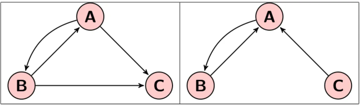
Figure 1.1: Illustrative examples of an undirected network, a directed network and a weighted network respectively.

1.2 From networks to complex networks

Thanks to the classical random graph model the structural properties, various characteristic quan-tities and even mechanism of network growth have been extensively studied analytically which required the graph to be simple enough to be handled rigorously. Most of the results were thus produced for undirected graphs such as simple graphs (graphs without multiplicity of links and without loops), regular graphs (graphs with same degree for all its vertices so that the degree distribution is a Dirac delta), tree graphs (graphs in which any pair of vertices is connected by a single unique path), complete graphs (graphs where each node is linked to every other node) or random graphs.

The random graph models are a statistical ensemble of all possible graphs that can be built with specific constraint such as a fixed number of nodes N or a fixed number of links L. The network is constructed by randomly assigning links to pairs of nodes, without entering into the details of these models, it is essential to note that as a result of this process the degree distribution p(k) follows a binomial law. Since the binomial law converges to Poisson law in the limit of large numbers, the

degree distribution p(k) of a random graph will tend to a Poisson distribution p(k) = e−¯k¯kk/k! in

the limit of large network size with ¯k being the average degree of a node.

In the late 1990s a revolution took place among the physicists in the network field when peo-ple started to study empirically real world networks such as the Internet and webpages networks [Albert et al., 1999]. It turned out that the degree distribution in those networks followed a power

law p(k)_{∝ k}−γ with the decay exponent being in the typical range of values 2_{≤ γ ≤ 3. Instead of a}

rapidly decaying distribution we have the so called fat-tailed distribution. This unexpected obser-vation triggered a lot of interest towards real-world networks rather than theoretical graphs and a great deal of different networks were found to be consistent with a fat-tailed distribution leading the community to investigate more deeply the topological properties of such systems[Caldarelli, 2007].

(10)

However because of statistical fluctuations it is difficult to assess a power law distribution on small networks, therefore it is safer to assume a power-law tendency in some cases.

Contrasting with the random graphs where the typical measure is the average degree of node, the networks following a power law distribution do not have a natural scale, hence the name

scale-free networks. This structural difference impacts drastically the behaviour and the organization of

such networks because of a large variety of node degrees and because of the presence of few crucial nodes called hubs which are a small number of vertices with a very high degree.

Fortunately already in the 1980s people started to push the mathematical model of random graph further, known as the configuration model, by generalizing it to an arbitrary degree distri-bution of nodes and gave one of the possible recipe to build such a random graph [Bollob´as, 1980]. This time to create one instance of the statistical ensemble we have to consider a set of numbers of

nodes{N(q)} of degree q and attach q half-edges to each node and then randomly connect them

by pairs until no more half-edges are left alone. This process recreates the classical random graph

ensemble if the values _{{N(q)} are drawn from a Poisson distribution and generates uncorrelated}

scale-free networks if the distribution used is a power law. Uncorrelated means that non trivial preferences of association between high degree nodes or a high and a low degree nodes are not captured by this model but still several features can be qualitatively explained only by the degree distribution.

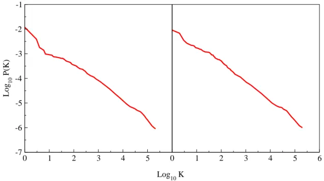
k

P(k)

Log k

Log P(k)

Figure 1.2: Illustrative examples of both types of graphs with their degree distribution below : a classical random graph (left) and a scale-free graph (right).

In addition to that improvement, to explain why such networks occur naturally in so many

different systems Barab´asi and Albert proposed a simple and elegant mechanism of scale-free

network formation and growth that is known today as the preferential attachment model and is generally considered as the most likely reason behind the structural organization of most real

world networks [Barab´asi and Albert, 1999]. The idea is that from an initial small set of nodes

we add one by one a new node which will be connected according to a specific rule so that when the number of nodes becomes larger and larger the degree distribution of the network tends to a power law. At a given time step the new added node is linked to an already existing node with a probability proportional to that node’s degree. The higher a node degree is the more it attracts new links from newly added nodes leading to the formation of hub like structures which in turn become ”centers” around which the network grows, hence the term ”preferential”.

(11)

networks [Watts and Strogatz, 1998]. The average shortest path length ¯l turned out to be quite a small number in comparison with the size of the network considered. This fact was expected but the idea that one can typically navigate in a huge network in a very limited number of steps is surprising. This feature is characterized by a logarithmic dependence of the average path length

with the network’s size ¯l_{∝ logN and is called the small-world effect which was nicely highlighted}

in an original social experiment conducted by Stanley Milgram in 1967 [Milgram, 1967].

Milgram wanted to study how closely people are related in the social network of acquaintances in the united states of America : He chose random people in the city of Omaha and a target man living in Boston. He gave letters to the people living in Omaha with the instruction that they should send the letter to the target man if they knew him directly or send it to someone, a messenger, who they think should be the most likely able to reach the target man but with the condition that they should know the messenger on a personal basis. After some time, some of the letters reached their destination and thanks to some tracking procedure Milgram observed that on average the letters went through five people before reaching the target man, hence the famous slogan ”six degrees of separation” explaining that on average anyone is quite close to anyone else even in a large population. This experiment has been widely criticized for lack of rigorous protocols and weak statistical significance, nevertheless it succeeded in capturing the essence of the small-world effect in an unexpected and funny way. The origin of the effect lies in the existence of links connecting distant parts of the network producing effective shortcuts in the overall organization of the nodes. In the scale-free networks that are also small-world the hubs are playing the roles of shortcut relays, effectively reducing the length needed to cross the network. On the contrary the networks that have specific constraint so that long distance connexions are impossible, due to the geographical distance in road network for instance, do not exhibit small-world properties.

scale-free small world directed

tree graph

Avian Influenza outbreaks X

Brainstem reticular formation X

C.elegans interactome X X

World Wide Web X X X

Table 1.1: Examples of networks that have been shown to be consistent with the three different specificities [Small et al., 2008, Humphries et al., 2006, Li et al., 2004].

It is clear that real-world complex networks show some common structural properties and non trivial behaviour which make them fundamentally different from classical random graphs. The massive shift of interest in the study of the former type of networks is understandable when we think about the wide variety of phenomenon that can be viewed as a system comprising nodes and links. Indeed the network approach offers the right amount of compromise between gener-alization and specificity, that is abstracting the actual objects represented by the nodes in or-der to find common features among globally different systems while keeping the complexity of the interactions and relationships between the objects. The possibilities of such an approach span several scales and areas and we can define networks for situations as diverse as in biol-ogy (gene regulation, protein interaction, neuron, metabolism, predation), in sociolbiol-ogy (relation-ship, acquaintances, groups), in IT (webpages, scientific citations, social medias), in infrastructure (cities agreement[Kaltenbrunner et al., 2014], transportations, banks, mobile relays) and even in unexpected areas such as linguistics and games (semantic[Corominas-Murtra et al., 2009], football games, tennis games[Radicchi, 2011], medieval history[Rodier et al., 2014]) and this list is of course far from being exhaustive.

In this thesis we will apply the Google matrix tools to complex networks defined for various situations such as the DNA sequences of several species, the neural system of the C.elegans worm, the ancient strategy board game called Go and compare them with previously studied networks such as university webpages or Wikipedia articles.

(12)

1.3 Tools to study the complex networks

The richness of the complex network approach opens up a lot of new questions and problems to be tackled in many different angles. Let us mention briefly without much details that there exist several well documented approaches such as the percolation theory which draws analogies with the behaviour of fluids filtering through a porous material, the compartmental models that are widely considered for epidemic spreading problems and so on, among them the linear algebra approach is of particular interest for us.

Matrix representation is a powerful tool to model finite size networks and characterize their topological features by spectral or eigenvector analysis. Typically a given static network of size N

is represented by a square matrix of size N × N where the nodes are labeled along the columns

and rows of the matrix so that the edges are given by the matrix elements. The adjacency matrix

A is a well-known example of such a representation where the elements aij = aji = 1 when the

nodes i and j are connected and aij = aji = 0 otherwise. This definition can be easily extended

to directed graphs by removing the symmetry aij = aji.

Other matrix representation variants include incidence matrix, degree matrix, Laplacian matrix and we will see in the next chapter that the Google matrix is constructed thanks to a variant of the adjacency matrix.

Centrality measures

In a given static graph we may wonder which vertices constitute the most crucial part of the network, for instance which ones are the most influential nodes, or which ones participate the most in the stability of the network and so on. To address those questions several quantities, called

centrality measures, have been proposed which allow us to determine quantitatively the relative

importance of the nodes within a network [Freeman, 1979]. Finding an appropriate centrality measure was in fact the key question asked by the founders of Google in the context of World Wide Web navigation.

The centrality is typically a real value, defined for a given node, which can be computed for every node of the system in order to compare their importance. Among the various measures the four main types are the degree centrality, the closeness centrality, the betweenness centrality and the eigenvector centrality.

The first one CD is defined as the degree of the node i, formally denoted by CD(i) = deg(i).

This is the most straightforward measure and translates a node’s importance simply to how many neighbours that node can directly affect (or be affected by) when the information flows through it.

The second one CC is defined thanks to the sum of the distances that separate a node i from

every other nodes, CC(i) = (Pjd(i, j))−1. The distance d is taken to be the shortest path and

this measure describes how far, in terms of number of steps, a node lies from all other nodes. This is therefore used to assert how long it takes for the information to reach the network from the considered node.

The third measure CB is defined for a give node i thanks to the shortest path lengths between

all the possible pairs of vertices :

CB(i) =

X

s6=i6=v σst(i)

σst

It considers the fraction of the shortest paths σ between two nodes that goes through node i

among all the shortest paths between them2_{. This fraction is computed for every possible pairs}

and summed up, this measure describes to what extent a node plays the role of relaying point. In practice the betweenness centrality is known to highlight nodes essential to the robustness of the network meaning that one can disrupt a system very quickly by removing the nodes in the order given by this measure.

2

A generalization based on random walk and including contributions of other than shortest paths is given in[Newman, 2005]

(13)

The last one is defined thanks to the matrix representation of a network and assigns a score to all the nodes so that the relative importance of each one of them can be deduced. This measure gives a higher score to the nodes that have connections to other high scoring nodes and helps to identify the most influential nodes in a given network. We will see in the following sections that the scoring system developed by Google is an eigenvector centrality measure.

Community structure

One of the most challenging analysis in the static network case is the detection of community structures. By community we mean a set of nodes, often referred to as a cluster in traditional network science terminology, that are more connected among themselves than to the rest of the network. Such a set of nodes form a group that might be interpreted in a concrete example as a class of objects with similar specificities[Girvan and Newman, 2002]. However there are no clear definition of the concept of communities and various algorithms have been proposed to detect such clusters (statistical inference, modularity maximization, clique based methods, ...) and some methods are tested on artificially produced communities so that it is still ambiguous and difficult to apply them in real life situations.

In [Fortunato, 2010] the author gives a complete overview of community detection techniques

discussing the main algorithms and explaining why the problem hasn’t been solved yet3. It is also

known that the problem is even harder for the directed network case nevertheless we will explore a possible way of extracting communities thanks to the Google matrix tool that could help us in providing a different insight on cluster organization.

1.4 Technical aspects and challenges in I.T networks

In parallel to the development of the graph theory, the second half of the XXth century had a

favourable political and historical context to intensifying scientific effort to materialize automated computing devices in order to perform mechanically or electronically tasks helping deciphering secret codes, encrypting communications, computing ballistics and so on. The theoretical founda-tions of logic and informatics were set by famous people like Alan Turing who introduced in 1936 a gedankenexperiment known later as Turing machine [Turing, 1937]. A Turing machine is an abstract model to implement a mechanical device to perform calculus following clear instructions depending on its state. Any problem that can can be treated with a clearly defined procedure solvable by a Turing machine means that a physical device, provided that it is powerful enough, can be built to solve it. On the contrary, there is no way of solving a problem if it is non solvable by a Turing machine.

This notion is thus an important precursor to the programming languages by providing a formal understanding of algorithms before the existence of actual computers and giving us an idea of what a computing machine should be to tell it apart from a simple automate. Besides the well known and advanced programming languages such as C/C++ (in which the simulations of this

work were done), anecdotically, the typesetting system LA_{TEXwith which this document is written}

is also equivalent to a Turing machine.

A few years afterwards several pioneers, among whom was the famous scientist John von Neumann, proposed a scheme for concrete realization of a fully functional computer which will be known as the von Neumann architecture [Burks et al., 1946]. To sum it up briefly this scheme suggested that a computer should be made of four parts : the arithmetic unit performing the basic operations, the control unit preparing the basic operations, the memory to register the program and the current ongoing operations and an input/output device to communicate with the external world.

3

(14)

Birth of the Internet

These foundational works greatly enhanced the technological development of the second half

of XXth century so much that research section of the USA defense agency promoted the

imple-mentation of efficient communication between their agents. The idea of communicating devices linked to each other through a standardised protocol is a precursor of the Internet. In the early 1990s the CERN came up with an elegant standard to access written documents but also image contents, videos and sound records that were addressed with a chain of characters known as URL and reachable through a browser [Berners-Lee, 1989]. The simplicity of the protocol along with the elaboration of tools to create such multimedia documents, called webpages, helped the growth and the popularization of the world wide web so much that estimates in 2013 put the number of

active websites to 5· 108 _{and the total number of webpages is perhaps ten times larger, at least}

for the indexed part of the Internet, leave alone the deep web.

The main success of the WWW nowadays comes from its numerous practical advantages over physical documents and its huge reservoir of knowledge accessible through not only computers but telecommunication devices as well. As the society tends to take the networking spirit even further with various enhancement of smartphone and mobile devices, signal processing technologies, cloud computing and so on it is crucial to come up with a profound understanding of the network properties and its behaviour.

Data challenge

Besides the intrinsic dynamical nature of the Internet which is in constant growth and un-dergoes constant modifications there is the fundamental question How do we efficiently retrieve

information ? Indeed one of the major task in such a huge evolving network is to navigate

effi-ciently in the ocean of webdocuments and find as quickly as possible the most relevant piece of information one is looking for. This question lead people to create search engines, software that use automated web crawlers to explore the WWW and collect information about webpages and their contents to build up a reference database from which a table of relevancy is constructed. Older versions of search engines worked on the basis of keywords query, that is, the database of indexed pages are analysed via their contents and a list of relevant words are registered so that each time somebody makes a query by typing one of the words, the search engine returns the webpages where these words appear frequently or in strategic positions such as titles and beginning of paragraphs. These methods, despite all the improvements one can make about extracting keywords and scoring webpages according to content, suffer from serious issues related to the human way of thinking and judging the importance of a document and also by the inability of our computers to process languages in a semantic level. It is a non trivial task to solve stemming problems and defining similar meaning words in a specific context, those similarities might be natural for us but hard to catch for an automated computer program which often show up as completely unrelated search results. This technique is also highly dependant on spelling specificities such as words which have almost same spellings, case sensitivity and so on. These failures motivated a novel approach to information retrieval that was by the way the basis for the success of Google [Langville and Meyer, 2006].

1.5 Google and network approach to information retrieval

The fundamental reason behind the difficulty to retrieve needed documents on the WWW is par-tially related to its structural organization. Indeed, unlike traditional archives such as libraries where files and books are arranged in a specific manner with categorization for providing a me-thodical and easy access to their content, there are no centralization nor any kind of hierarchy within the Internet. To circumvent all these limitations it was necessary to approach the webpages

(15)

scoring problem from a different angle. Instead of relying solely on the content of the webpages, one can try to look at the network perspective of interconnected web documents and ask the question

What are the most important webpages corresponding to a given query ? In addition to suggesting

a couple of websites and listing them in order of importance, this centrality oriented method should also correspond to how human web users define the importance of a website. Indeed the average user relies on the first results returned by a search engine and usually does not bother to look further in the listing.

During the years 1995 and 1996, two PhD students in Standford University, Sergey Brin and Larry Page, met and came up with a brilliant idea of assigning a recursively computed score to list the webpages in order of importance that happens to correlate well with what people expect about a website’s relevancy to answer their queries [Page et al., 1999]. This method, called the PageRank

score, is based on the point of view that a hypertext link (link that people put in their websites

as suggestions for visiting related or complementary materials or for reference materials) is some kind of recommendation system. In a sense if many people put a link from their webpages towards a particular website it means that they consider that one as a relevant source of documentation and worthy to be visited. Therefore the more a website has incoming links the more it is popular or important. The recursion is taken into account by the fact that the score of a website is higher if other important websites (with a high score themselves) point to it. Similarly the weight of a recommendation (a hypertext link) of a website is decreased if it tends to point to many other websites because the value of its recommendation would be lower. Another drastic advantage of considering such incoming links is that one cannot easily fake one’s own website importance by artificially boosting the score which is also the reason why outgoing links are discarded in this analysis.

Around the same time a very similar conceptual approach was proposed by Jon Kleinberg in the form of HITS algorithm [Kleinberg, 1999]. This query dependant method is sometimes considered as a precursor of PageRank scoring system as it assigns a pair of values called hub and

authority scores to the nodes of a network (webpages) based on their ingoing and outgoing link

structures. A high hub score indicates a node pointing to many other nodes and a high authority score indicates a node pointed by many hubs. Similarly to the PageRank score, HITS values are computed recursively but using mutually the ingoing links and the outgoing links. This dependence on outgoing links and on the query eventually made PageRank algorithm preferred over HITS.

At the end of their PhD thesis Brin and Page became the founders of Google the now multi-million dollars company dominating various aspects of the Internet world in terms of search perfor-mance and information providing services[Ginsberg et al., 2009, Preis et al., 2010]. Even though to this day several dozens of equally important factors are taken into account by their search engine in order to provide a high quality tool, the idea of PageRank scoring was and still is at the core of its success thanks to its easy computability and efficient results making it a good compromise between relevancy and computing cost and therefore rendering it applicable to the evergrowing World Wide Web. On a funny ending note the name Google originates from a misspelling of the

word Gogol representing the huge number 10100 probably as a metaphor for the huge database

that Google can handle and the PageRank scoring is a word play using ”webpage score” and the last name of Google’s co-founder Larry Page.

1.6 Aim of the thesis

This chapter presented a brief overview of some basic concepts about the complex networks and grasp the main developments that lead to modern day information technologies and the related challenges. The founders of Google developed a highly efficient and promising tool to study the topology of large scale-free directed networks. As it works well with the webpages network, one can expect these tools to yield interesting results and shed a new light on various real-life systems that can be viewed as a directed network. In the next chapter we are going to present the mathematical theory behind the PageRank scoring system which can be viewed as an eigenvector of a matrix

(16)

called the Google matrix. We will see how to construct this matrix and discuss its eigenvalues and eigenvectors properties in chapter 2. In the following chapters 3, 4 and 5 we will discuss those properties in more details by applying the Google matrix analysis on some concrete examples of real world systems. It will in the same time bring the reader in a journey from small scale to large scale systems illustrating how network theory can be broadly used to gain some insight in many different situations. Before concluding this work, in chapter 6 we will discuss the use of PageRank in a different context related to the field of socio-physics and opinion formation study.

(17)

Chapter 2 The Google matrix

2.1 A brief reminder about Markov Chains

Before diving into the mathematics of the PageRank scoring system, which is a probability distri-bution vector, let us briefly explain the very closely related model of Markov chains. This tool of probability theory was developed around 1906 by the great Russian mathematician Andrei Markov to describe stochastic processes undergoing transitions [Markov, 1906]. Markov models have been extensively studied and found many applications in areas such as physics, biology, statistics and finance. Among the variants of the models, we will concentrate on the simplest of them : discrete-time finite state space homogeneous Markov chain.

Formally a Markov chain is a sequence of random variables X0, X1, X2, ... having the so-called

Markov property, meaning that the probability of the future event Xt+1depends only on the current

state Xt and not on the history of the sequence. This property is also referred to as memoryless

process explicitly given by :

P r(Xt+1= x|X1= x1, X2 = x2, ..., Xt= xt) = P r(Xt+1= x|Xt= xt) (2.1)

The indices 1, 2, ... is generally considered to label the time evolution and here it describes the state of the system at discrete time steps. The outcomes of the random variables are called states and the set S of all possible states is called the state space, which will be considered finite in our case.

If the system is evolving between a fixed number of states N , the stochastic transitions can be

represented by a matrix P of size N× N whose elements Pij = P r(Xt+1 = j|Xt= i) describe the

transition probability from state i towards state j. By definition the elements are non negative with

0_{≤ P}ij ≤ 1 and the sum of the elements along each row of P is equal to onePiPij = 1 therefore

the matrix P is said to be row-stochastic. If the conditional probabilities do not depend on the

position along the sequence, that is if the matrix elements Pij are independent of the time steps t,

the Markov model is said to be homogeneous. Such a Markov process is very often schematically represented by a directed graph (cf. Fig 2.1).

One of the most crucial notions in the Markov chain model is the limiting behaviour of the random variable sequence. The limiting distribution π is a row vector of the same size as the state space and whose entry i corresponds to the time that the system spends in state i in the long run, which is expressed as : π(i) = lim t→∞ 1 t t X j δ(Xj, i) (2.2)

If such a limit exists, after the proper normalizationP

iπi= 1, it is considered as a stationary

probability distribution meaning that the measure π is left invariant by the transition matrix

π = πP . Alternatively we can look for this invariant measure by solving the eigenvector equation

(18)

P =





A B C A

0

0 .7 0.3

B

0 .4 0.3 0.3

C

0 .4

0

0 .6





A

B

C

0.3 0.7 0.4 0.3 0.3 0.6 0.4

Figure 2.1: Illustrative example of a matrix representation of a 3 states homogeneous Markov chain with its directed graph representation.

The study of stationarity is closely related to the concept of first return time Ti which is

the step when the Markov process returns back to the state i for the first time after having left it

previously. Considering the lower bound of the ordered sequence of random variables X0, X1, X2, ...

we have that Ti = inf{t ≥ 1 : Xt = i|X0 = i}. The set of first return times Ti are also random

variables and the quantity P r(Ti = t) describes the probability that the Markov process starting

from state i returns to state i after t iterations. If there is a finite probability P r(Ti = +∞) > 0

that the system will never return to state i, that is if P∞

t=1P r(Ti = t) < 1 the state i is called transient. Otherwise it is called recurrent and if all states are recurrent the Markov chain is said

to be recurrent.

Moreover if the expectation of the first return time of state i is finite Ei(Ti) < +∞, the state

i is called positive recurrent. Similarly if all states share the same property the Markov chain is

said to be positive recurrent.

One more useful definition is the period k of a state i which is nothing more than the greatest

common divisor of the set of recurrence times k = g.c.d.{t : P r(Xt= i|X0 = i) > 0}. If the state

i occurs at irregular times, k = 1 and the state is aperiodic.

There are several ways to determine the existence of a stationary state, the one that we are interested in involves the notion of irreducibility. A Markov chain is said irreducible if there exist

an integer t > 0 such that P r(Xt = j|X0 = i) = Pij(t) > 0 for any pair of states i and j, in other

words if there exist a probability of transition from any state i to any state j.

In terms of directed graph representation this requirement translates into the graph associated to the transition matrix P being strongly connected, meaning that for each pair of vertices (i, j) there is a path going from i towards j.

With those concepts, an important theorem states the existence of a stationary probability distribution which is by the way the root of the existence and unicity of the PageRank vector.

Every irreducible Markov chain with a finite state space is positive recurrent, thus having a unique stationary distribution π. And if the chain is aperiodic, π is the limiting

distribution π = limk→∞P(k)v for any probability distribution v.

Theorem 1 (Existence and unicity of stationary state).

Random walk on graphs

A random walk is a mathematical description of a path formed by some stochastic process and modeled by random steps. Such a model is helpful to study complicated dynamical processes that look random but might not be so in reality such as stock market fluctuations or molecules

(19)

trajectories and they are usually represented by a Markov chain. Random walks can be per-formed on various objects such as a line, a plane or even on mathematical objects such as graphs [Rudnick and Gaspari, 2004].

The original idea of the PageRank inventors was to consider an Internet user as a random walker on a large network. The web surfer visits some webpages and clicks randomly on a hypertext link listed on the current website he is looking at. He does so at each step which can be a rough but still decent approximation to the average behaviour of human Internet users. Indeed usually people tend to navigate on the web following some links from the webpage they are currently looking at and in general this choice is unrelated to the websites visited previously. If we imagine a random surfer moving across the network at each step for sufficiently long time it will eventually revisit some webpages several times. We can interpret those webpages as important ones because they have many incoming links from other important websites and in the long run the time that the random surfer spends on each site would determine their relative importance. The PageRank scoring system is thus seen as one of the greatest applications of the Markov chain theory through the imagery of a random walk on a complex network.

We mentioned earlier that disabling the nodes following the betweenness centrality order rapidly destroys the network, in fact removing the nodes following the PageRank order is also quite an efficient way of disrupting the network. However contrary to the first centrality measure the PageRank measure is much more easier to compute as we will see in the following sections.

2.2 Summation formula of PageRank

Let us get back to the network science with a surprising anecdote, Brin and Page’s first papers about their search engine did not even mention Markov chain models. Not knowing the strong connection between their PageRank scoring method and the Markov chain they derived a summation formula to assess a score of a webpage by analysing the structure of academic papers citations network [Langville and Meyer, 2006]. Their idea is that the PageRank score p(i) of a website i should be the sum of all PageRank scores of websites pointing to i.

p(i) = X j∈Bi

p(j)

|j| (2.3)

where Bi is the set of websites pointing to i and |j| denote the number of total outgoing links

from webpage j. This summation formula requires the unknown score of neighbouring webpages, to overcome this problem they rendered the formula iterative :

pt+1(i) =

X

j∈Bi pt(j)

|j| (2.4)

so that the scores which are computed for each webpage at step t use the scores computed

previously at step t− 1, starting from an initial distribution of values p0 which can be set for

instance to the uniform vector p0(i) = 1/N ∀i with N being the number of websites indexed by

the search engine.

From this point on we can naturally wonder if the iterative process does always converge or not, if the convergence is fast or slow and if the final PageRank vector is unique or depends on the initial values. In fact there are several situations leading to convergence problems (cf. Fig 2.2) in this iterative process, for example when the random surfer falls in a particular site with no outgoing links, called a dangling node, it stops there meaning that at each computing iteration that particular node absorbs more and more probability falsely increasing its PageRank score. Because of that behaviour, those nodes are sometimes referred to as rank sink and they are quite common on the Internet especially when we consider that many webpages have links to downloadable documents and multimedia contents that lead to nowhere.

(20)

A

B

C

A

B

C

Figure 2.2: Simple examples of rank sink : node C is a dangling node (left), nodes A and B form a dangling group (right).

In addition to that there is also the case of a cluster of webpages with internal links only among themselves, in which case the random surfer gets trapped in an area formed by a subset of sites from which it cannot escape. To understand these issues mathematically we will switch to a matrix representation of the summation formula and give the recipe to carefully handle the modifications at the end of which the resulting matrix is the Google matrix, thereby ensuring the existence and unicity of the PageRank vector to which any initial distribution will converge.

2.3 How to construct the Google matrix ?

Throughout this section we will discuss the construction of the Google matrix G using a simple toy model example of a small directed graph pictured in Fig. 2.3, the recipe for larger networks is exactly the same.

1

2

3

4

5

6

7

8

Figure 2.3: Directed graph used to illustrate the construction of the Google matrix G in this section. Probability absorbing areas (rank sink) are shaded in gray.

1 : Asymmetric adjacency matrix

The first step consists of building the matrix A which describes the connectivity structure of

the directed network. It will be an asymmetric matrix of size N _{× N where N is the number of}

(21)

in columns or in rows, here we use the column labels to designate the origin of a link and the row

to designate the destination so that the matrix elements Aij = m if there are m links from node

j pointing towards node i where m is an integer number representing the multiplicity of the link

and Aij = 0 otherwise. In our toy model we don’t have multiple links, so m = 1 and the matrix

corresponding to the network in Fig. 2.3 reads :

A =               0 0 0 0 0 0 0 0 1 0 0 1 0 0 0 0 1 1 0 0 0 0 0 0 0 1 0 0 0 0 0 0 0 0 0 1 0 0 1 0 0 0 0 1 1 0 0 1 0 0 0 0 1 0 0 1 0 0 0 0 1 1 1 0               (2.5)

Next we need to normalize the columns to one so that the matrix becomes similar to the transition matrix of a Markov chain. The elements would be the probability of getting from a

node to another one and the matrix vector product using A′ is the transcription of the summation

formula in eq. 2.4 : A′ =               0 0 0 0 0 0 0 0 1/2 0 0 1/3 0 0 0 0 1/2 1/2 0 0 0 0 0 0 0 1/2 0 0 0 0 0 0 0 0 0 1/3 0 0 1/2 0 0 0 0 1/3 1/3 0 0 1/2 0 0 0 0 1/3 0 0 1/2 0 0 0 0 1/3 1 1/2 0               (2.6)

The physical motivation behind column normalization is that we want to treat all the outgoing flows on the same footing so that comparisons between nodes capture mostly their efficiency of connections rather than their volume of connections.

2 : Handling the dangling nodes

In the next step we have to deal with the dangling nodes that attract all the probability upon

themselves. Those nodes are columns full of zero in the matrix A′ because they are precisely the

vertices without any outgoing links. Mathematically we need to render the A′ matrix stochastic

therefore the columns of zeros are replaced with columns of 1/N where N = 8, in our case, is the

size of the system. Formally we then have the stochastic matrix S = A′+ (1/N )edT where e is

the column vector of ones and d the column vector whose entry d(i) = 1 if node i is a dangling node and d(i) = 0 otherwise.

Physically the interpretation of this trick is that virtual links are put from the dangling node towards every other nodes of the system so that when the random surfer falls into the rank sink it will then go randomly and with equal probability to any other part of the network. Regarding our behaviour as Internet users it still makes sense as once we hit a link to download a pdf file for example we will then visit a totally different website.

For our example of Fig. 2.3 where the vertice number 3 is a dangling node, the stochastic matrix S now reads :

(22)

S =               0 0 1/8 0 0 0 0 0 1/2 0 1/8 1/3 0 0 0 0 1/2 1/2 1/8 0 0 0 0 0 0 1/2 1/8 0 0 0 0 0 0 0 1/8 1/3 0 0 1/2 0 0 0 1/8 1/3 1/3 0 0 1/2 0 0 1/8 0 1/3 0 0 1/2 0 0 1/8 0 1/3 1 1/2 0               (2.7)

Sometimes this matrix is used as the Google matrix however in this form we are still not guaranteed to converge towards the PageRank in the most general case.

3 : Handling the dangling group

In the final step, we have to deal with areas of the network where the random surfer cannot escape from. Those groups of nodes can have connections among themselves but none of them have connections getting out of the group as shown in our example by the large grayed area in Fig. 2.3. Mathematically the problem arises because S is not guaranteed to be primitive. A non-negative

square matrix M is said to be primitive if there exists an integer k > 0 such that Mk

ij > 0 for all

pairs (i, j). To fix this property we need to add a dense rank one matrix traditionally denoted by

E and usually taken to be E = (1/N )eeT. The final form of the Google matrix G is a linear sum of this matrix E and the stochastic matrix S :

G = αS + (1_{− α)} 1 Nee

T _(2.8)

where α is an arbitrary parameter, called the damping factor, taken in the range 0_{≤ α ≤ 1 so}

that with probability α the transition between node j towards i is described by the structure of the

network and with probability 1− α the transition from node j towards any other node is rendered

possible with equal probability. In our example, the Google matrix associated to the network in Fig. 2.3 reads with α = 0.8 :

G =               1/40 1/40 1/8 1/40 1/40 1/40 1/40 1/40 17/40 1/40 1/8 7/24 1/40 1/40 1/40 1/40 17/40 17/40 1/8 1/40 1/40 1/40 1/40 1/40 1/40 17/40 1/8 1/40 1/40 1/40 1/40 1/40 1/40 1/40 1/8 7/24 1/40 1/40 17/40 1/40 1/40 1/40 1/8 7/24 7/24 1/40 1/40 17/40 1/40 1/40 1/8 1/40 7/24 1/40 1/40 17/40 1/40 1/40 1/8 1/40 7/24 33/40 17/40 1/40               (2.9)

The added matrix E is called the teleportation matrix thanks to its effect on the random surfer. Whenever the surfer gets trapped inside a dangling group, now it still has a non zero probability to jump elsewhere in the network thereby continuing its network exploration. It is a common image to mentally represent the flow of probability in the network and to obtain a stationary distribution it is essential that the whole network is continuously explored.

There is also a natural argument in favor of the teleportation matrix when we consider the be-haviour of actual people surfing the Internet, usually when they get bored of following a particular thread they will start to look for a different topic, modify their queries and start surfing again in some other part of the WWW network.

(23)

Perron-Frobenius operators and dominant eigenvector

In the form of eq. 2.8 the Google matrix G is stochastic, irreducible and aperiodic which in the context of Markov chain theory (cf. theorem 1) ensures the existence and the unicity of a stationary probability distribution : the PageRank vector. Indeed thanks to its definition, G belongs to the class of so called Perron-Frobenius operators therefore the famous Perron-Frobenius theorem (cf. theorem 2) applies to it, consequently ensuring that a unique strictly positive eigenvector exists [Perron, 1907, Frobenius, 1912]. This theorem has several statements, here are some of them that are directly interesting for us :

Let A be a primitive matrix

• The spectral radius r = ρ(A) is a simple eigenvalue of A. • ρ is the only eigenvalue on the spectral circle of A.

• There is a unique eigenvector v such that Av = ρv and vi> 0 ∀i.

Theorem 2 (Perron-Frobenius Theorem).

We can now confirm that the spectral radius ρ of the Google matrix G is equal to one which

is also the dominant eigenvalue λ1 = ρ = 1. Since G is asymmetric the eigenvalues are complex

valued and distributed on the complex plane inside the unit circle. The eigenvector v corresponding to the eigenvalue λ = 1 satisfies Gv = v and has all positive entries.

This vector can be normalized as p = v/P

ivi so that the sum of its entries add up to one, the

resulting vector p is called the PageRank vector and has a meaning of a probability distribution over the nodes of the considered network. To derive a ranking from this probability distribution, since by definition the PageRank vector is positive definite, we can rearrange its elements p(i),

through a permutation σ(K) = i, in decreasing order to obtain a list of values p(K) so that p(K1) >

p(K2) > ... whose indices Ki denote the rank of the nodes such that low values of K = 1, 2, .. mean

a high ranking thus indicating very important nodes. The normalized vector corresponding to our

little example in eq. 2.9 is pT _{= (0.0318, 0.0594, 0.0683, 0.0556, 0.1187, 0.1948, 0.1800, 0.2914) which}

can be reordered decreasingly with the following permutation σ = (8, 7, 6, 5, 3, 2, 4, 1). The most

important node, the most highly ranked is K1 = 8 followed by K2 = 7 and so on.

The word PageRank is sometimes used ambiguously to designate the actual value or the rank-ing, to avoid any confusion we will refer to the probability distribution vector as PageRank vector and the ranking of its elements as PageRank indices.

PageRank vector numerical computation

The PageRank computation can be stated as the following eigenvector problem for p with the

normalization constraintP

ipi = 1 :

Gp = p (2.10)

When dealing with relatively small size systems (N . 104) where the whole matrix G can be

stored and handled easily, it is straightforward to diagonalize the matrix and obtain the

eigenvec-tor corresponding to λ1 = 1. However for the huge networks such as the WWW handling and

performing operations on the whole matrix is not feasible and the memory requirement would be far off the technical limitations.

(24)

An interesting alternative would be the power method which is an iterative method and one of the several numerical recipe used to find the stationary solution of a Markov chain[Stewart, 1995, Mises and Pollaczek-Geiringer, 1929]. Among all the methods to find the dominant eigenvector of a matrix, the power method is the simplest one and the easiest to implement making it the favorite candidate in PageRank vector computation despite its well-know algorithmic slowness. So what advantages does the power method give to be still interesting today ? The answer is threefold : First, in the context of WWW network it is suited to the sparse structure of the normalized adjacency matrix, second it has a linear complexity and converges quickly in some cases and third it is a matrix-free method.

Matrix sparsity

A matrix which has a large proportion of its entries equal to zero is said to be sparse, otherwise it is said to be dense and the fraction of non zero elements in the matrix is called the sparsity. For the general case there are no clear definition of the sparsity in the literature

as this notion is used qualitatively in most cases1_.

This notion is important in numerical computing as there exists several methods accelerating and improving the efficiency of computations when applied to sparse matrices. Moreover there are specific sparse matrix representation formats which stores the minimal needed information content of the matrix by disregarding all the zero entries consequently saving a lot of memory space and thus allowing for larger matrix computations. In the case of the World Wide Web network, the matrix describing the connectivity structure would be huge in

size, about 108_{× 10}8_{, but on average a typical webpage has about}_{≈ 10 connections towards}

other websites making the number of non zero elements to be about ≈ 109 _{so that their}

fraction is about≈ 10−7 _{which is extremely sparse.}

Algorithmic complexity

Computational complexity theory studies the intrinsic properties of mathematical problems and classifies them according to their difficulty [Arora and Barak, 2009]. The notion of big

O is used to denote the asymptotic speed behaviour of an algorithm in an arbitrary unit of

time in the worst case scenario. The complexity is usually expressed with the size of the input data n and gives the time needed for the algorithm to terminate in the case that all the computations must be done (disregarding simplifications and shortcuts due to a specific

problem). For example if an algorithm has a complexity of O(n2) it means that if we give a

two times larger dataset as an input to be processed, the algorithm will take four times longer to run and terminate on the same machine. There are many different behaviour such as the constant complexity, denoted by O(1), meaning that the size of the input data is irrelevant to the computation duration or the linear complexity, denoted by O(n), meaning that the runtime is proportional to the data size. Naive coding and simple solutions often results in high complexity, if we wish to optimize an algorithm it is crucial that we try to reach the lowest possible complexity.

Due to the peculiarities of the Google matrix, especially in the case of a sparse network, the eigenvector problem stated in eq. 2.10 can be rewritten thanks to the sparse connectivity matrix

A′ as :

pt+1= Gpt= αA′pt+ (αdTpt+ 1− α)e/N (2.11)

where d is as before the vector indicating the dangling nodes. In order to compute the eigen-vector at step t + 1 we need to know it at step t and since the stationary solution is unique we

1

However in the context of graph theory a rigorous measure is suggested in [Randi´c and DeAlba, 1997] in the form of compactness ρ = 2en/((n − 1)(n2

− 2e)) for simple undirected graphs with n vertices and e edges. As there cannot be a graph with ρ = 1, if ρ < 1 the graph and the corresponding adjacency matrix are sparse and if ρ > 1 they are dense. A similar argument can be derived for simple loopless directed graphs.

(25)

end up on the same vector whatever the initial probability distribution chosen at t = 0, usually

the uniform vector p0 = (1/N )e is used.

Despite the fact that the indexed webpages are growing in number there are in principle no reason for the average number of connections per page to change much. It is safe to assume

that one iteration with A′ matrix is similar to a matrix vector product where the number of

non zero elements in each row of the matrix is bounded by a constant C ≪ N. In such a case

the complexity of one iteration step is O(n) linear and therefore the computation is quite fast. Moreover the whole procedure does not require the handling of the whole Google matrix, indeed

only the sparse representation of A′and the current iteration of the vector ptare stored in memory.

Finally Brin and Page originally stated that only about 50 to 100 iterations are enough for the level of precision needed for website indexation.

In practice the Internet is constantly evolving and growing so that a real time PageRank computation is practically impossible, instead Google is using huge servers to crawl the web and perform the computations once every two or three months to update the score of all the webpages.

2.4 Spectrum and PageRank properties

Eigenvalue spectrum properties

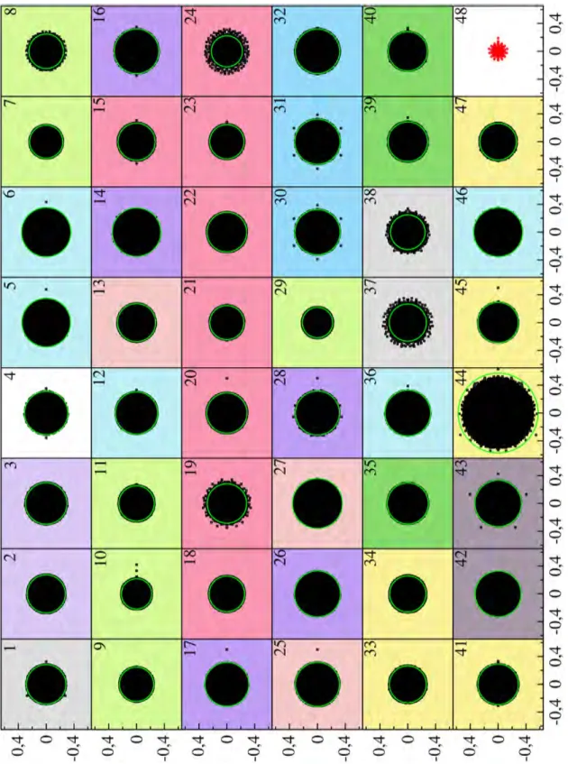
As mentioned earlier the directed network description makes the Google matrix asymmetric, therefore the matrix diagonalization produces complex conjugated pairs of eigenvalues that are distributed inside the unit circle in the complex plane (cf.theorem 2). As we will see in chapter 3 the eigenvalue cloud in itself provides some insight regarding the structural properties of the considered network and in chapter 5 we will discuss the next to leading eigenvalue and their ties to the community structures.

In Fig. 2.4 two concrete examples of spectrum of the Google matrix are shown for university

websites in 20062 where some of the largest eigenvalues of the webpages of Cambridge university

(left panel) and Oxford university (right panel) are displayed [Frahm et al., 2011]. This might seem to be a little restrictive to represent the entire World Wide Web nevertheless both of these networks are already very large with respective sizes of N = 212710 and N = 200823 nodes for Cambridge and Oxford, they also show scale-free behaviour and small world property. Moreover

they show a sparse structure with a respective number of directed links of Nl = 2015265 and

Nl= 1831542 which is about≈ 10 connections per node for both of them.

Effect of α damping factor : These spectrum (in Fig. 2.4) were computed at α = 1 which

is technically the spectrum of the stochastic matrix S. However both the spectrum of S and of G are very closely related by the damping factor α as stated in theorem 3. This parameter determines to what proportion the Google matrix describes the actual network structure and the random hopping term and effectively scales all but the leading eigenvalue of S irrespective of the specificities of the teleportation matrix. The scaling introduces a spacing between dominant and

next to dominant eigenvalues_{|λ1| − |λ2| which is called a gap in physicists terminology.}

If the spectrum of the stochastic matrix S is_{{1, λ1}, λ2, ..., λN}, then the spectrum of the

Google matrix G = αS + (1− α)evT _is _{{1, αλ1}_{, αλ}

2, ..., αλN}, where vT is a probability

vector.

Theorem 3 (Eigenvalue relations).

In the case where the gap is arbitrarily small or nonexistent (as in Fig. 2.4), that is when the spectrum shows eigenvalues very close to the unit circle in the complex plane, the system possesses

2

(26)

-1 0 1 -1

0 1

-1 0 1

Figure 2.4: Spectrum of the Google matrix at α = 1 for Cambridge university website (left panel) and Oxford university website (right panel). Not all the eigenvalues are displayed here and the plots are made with data from [Frahm et al., 2011].

distinct independent regions which are weakly linked to the rest of the network. If the eigenvalues are strictly located on the unit circle, the parts are disjoint which is mathematically expressed as a reducible system in which case the introduction of the teleportation matrix will connect those disjoint parts together by introducing a spectral gap.

Invariant subspace decomposition : To gain a deeper insight about those eigenvalues

located around the unit circle, it is useful to consider the invariant subspace decomposition. In the typical WWW like networks the nodes can be separated into two subsets : core space nodes and

subspace nodes. The first group constitutes the larger part of the network containing all the nodes

from which every other nodes are reachable in a finite number of steps. If we explore the network in the same way starting from a node belonging to the second group we will eventually get stuck inside a small subset of nodes that form what is called an invariant subspace that is in fact left invariant with respect to the application of S. This separation allows to rewrite the S matrix in a

block triangular form S = SSS SSC

0 SCC

!

because it is possible to enter in a subspace from the core

space but not possible to escape from a subspace. The subspace part SSS itself can be composed of

several invariant subspaces and therefore made of diagonal blocks of various dimensions which are each a Perron-Frobenius matrix thereby producing at least one eigenvalue λ = 1 for each block.

The size of the subspace part depends on the system but the distribution of the various sub-spaces size seems to follow an universal function. These properties along with the detailed algo-rithm to construct the core space and subspace are discussed in [Frahm et al., 2011].

PageRank properties

In Fig. 2.5 we show the PageRank probability vectors, eigenvectors of the Google matrix at

λ = 1, computed for both Cambridge (left panel) and Oxford (right panel) university webpages.

The plot shows that in logarithmic scales the probability distributions, when ordered decreasingly, have a consistent linear behaviour over a wide range of values meaning that the PageRank values

Application of the Google matrix methods for characterization of directed networks

TH `

ESE

TH `

ESE

DOCTORAT DE L’UNIVERSIT´

E DE TOULOUSE

Acknowledgements

Contents

Chapter 1

Introduction

1.1

What is a Network ?

1.2

From networks to complex networks

1.3

Tools to study the complex networks

1.4

Technical aspects and challenges in I.T networks

1.5

Google and network approach to information retrieval

1.6

Aim of the thesis

Chapter 2

The Google matrix

2.1

A brief reminder about Markov Chains

P =





0

0

.7 0.3

0

.4 0.3 0.3

0

.4

0

0

.6





A

B

C

2.2

Summation formula of PageRank

A

B

C

A

B

C

2.3

How to construct the Google matrix ?

1

2

3

4

5

6

7

8

2.4

Spectrum and PageRank properties