Solar simulation test up to 13 solar constants for the thermal balance of the Solar Orbiter EUI instrument

Solar simulation test up to 13 solar constants for the thermal balance

of the Solar Orbiter EUI instrument

Laurence Rossi

and Maria Zhukova

and Lionel Jacques

, Jean-Philippe Halain

, Marie-Laure

Hellin

, Pierre Jamotton

, Etienne Renotte

, Pierre Rochus

, Sylvie Liebecq

, Alexandra Mazzoli

a

Centre Spatial de Liège, Université de Liège, Liege Science Park, 4031 Angleur, Belgium,

http://www.csl.ulg.ac.be/

ABSTRACT

Solar Orbiter EUI instrument was submitted to a high solar flux to correlate the thermal model of the instrument. EUI, the Extreme Ultraviolet Imager, is developed by a European consortium led by the Centre Spatial de Liège for the Solar Orbiter ESA M-class mission. The solar flux that it shall have to withstand will be as high as 13 solar constants when the spacecraft reaches its 0.28AU perihelion.

It is essential to verify the thermal design of the instrument, especially the heat evacuation property and to assess the thermo-mechanical behavior of the instrument when submitted to high thermal load.

Therefore, a thermal balance test under 13 solar constants was performed on the first model of EUI, the Structural and Thermal Model. The optical analyses and experiments performed to characterize accurately the thermal and divergence parameters of the flux are presented; the set-up of the test, and the correlation with the thermal model performed to deduce the unknown thermal parameters of the instrument and assess its temperature profile under real flight conditions are also presented.

Keywords: Sun simulator, Solar Orbiter, solar constant, thermal balance. 1. INTRODUCTION 1.1 Solar Orbiter and EUI instrument[1]

Solar Orbiter is a mission dedicated to solar and heliospheric physics. It was selected as the first medium-class mission of ESA's Cosmic Vision 2015-2025 Programme. It will be launched in 2017 (baseline) and is devoted to solar observation from an elliptical orbit around the Sun approaching to 60 solar radii. It will provide unprecedented close-up and high-latitude observations of the Sun.

The EUI instrument is composed of two high-resolution imagers (HRI), one at the hydrogen Lyman-α line (HRILya) and

one in the extreme ultra-violet (EUV) at 174 Ǻ (HRIEUV); and one dual band full-sun imager (FSI) working alternatively

at the two 174 Ǻ and 304 Ǻ passbands.

EUI is a compact instrument based on a passive thermo-mechanical design (no active control and passive detector cooling) taking advantage of a low CTE optical bench on which the three EUI channels are mounted and co-aligned.

1

1.2 In-flight thermal environment of EUI[4]

EUI is an internally mounted unit and therefore thermally linked to the spacecraft TCS (Thermal Control Subsystem). EUI is protected from the major sun heat input by the spacecraft heat shield. The HRI (High Resolution Imager) reflective entrance baffles reject more than 50% of the light coming through the entrance pupils. The FSI (Full Sun Imager) entrance baffle absorbs the minor heat load incoming through its small entrance pupil. The entrance baffles, filter and door assembly will receive an additional IR heat load from their respective HS (Heat Shield) feedthrough that are hotter. Most of the IR and visible heat load affecting the HRI entrance baffle assemblies is dissipated to space via a Hot Element (HE) interface provided by the S/C. The heat is conducted from the entrance baffles assemblies to the HE interface by means of two heat pipes in parallel. The detector cooling (at -40°C with target at -60°C) is achieved via a Cold Element (CE) interface combined with a Medium Element (ME) interface both provided by the S/C. The ME allows reducing the camera Front End Electronics (FEE) heat load onto the detectors and to reduce the FEE temperature. There are five major thermal interfaces between Solar Orbiter spacecraft and EUI instrument as shown on figure 1:

1. The spacecraft structure, providing a radiative environment for the EUI housing and a conductive interface for the EUI mounts.

2. The S/C heat shield feedthroughs, providing a radiative environment (with a positive IR heat input) for the entrance baffles.

3. 2 cold element (CE) interfaces, one providing the conductive cooling of both HRI detectors and the other of the FSI detector.

4. 2 medium element (ME) interfaces, one providing the conductive cooling of both HRI FEE and the other of the FSI FEE.

5. The hot elements (HE) interface, providing a way to evacuate the visible and IR heat absorbed by the HRI entrance assemblies.

Figure 1: EUI thermal interfaces

1.3 First model of EUI: the structural and thermal model[1]

The EUI model philosophy is summarized in table 1. It is organized around four models that will be manufactured and tested: one structural and thermal model (STM), one engineering model (EM), one qualification model (QM) and the flight model (FM). The structural and thermal model was tested during this thermal balance.

S/C structure S/C Heat Shield S/C heat shield Feedthrough Honeycomb bench HRI FPAs FEE APS OBS CEB HE CEHRIs MEHRIs

HRIs Entrance baffle, door, filter assembly

FSI FPA CEFSI MEFSI URP1 URP2 SRP Radiative environment QS QB FEE APS

Table 1: EUI model philosophy

Model Objectives Representativity

Structural & Thermal Model

(STM) 

validation of thermal design and math models

 validation of structural design (primary structure) and math models

 to derive subsystem environmental specifications

 mounting interface

 mass properties

 structural properties

 thermal properties

 envelope and shape

 subsystems structural & thermal dummies

 interconnecting harness

Engineering Model (EM) _ validation of functional interfaces

 validation of TM/TC protocols

 validation of operational procedures

 electronics with flight layout with respect to electrical parameters but populated with lower-grade parts

 subsystems electrical dummies

 interconnecting harness

Qualification Model (QM) _{ verification of integration and alignment plans}

 end-to-end verification of optical paths

 verification of electrical performances, incl. EMC

 validation of on-board software and functional interfaces

 instrument qualification

 flight-like optics

 functional sub-equipments dummies for redundant/recurrent sub-equipments

 full flight design & flight standard with respect to electrical parameters

Flight Model (FM) _ flight use  full flight design & flight standard

Flight Spare (FS)  flight use (spare)  full flight design & standard

 refurbished EQM

 electronic spare parts

The STM of EUI is shown on figures 2 and 3, without MLI:

Figure 21: EUI STM (without MLI) Figure 32: EUI STM (without MLI) without _{the top panel}

The sub-systems of the EUI STM are thermally and mechanically representative of the flight model. The mirrors are flat mirrors to allow theodolite measurements before, during and after the thermal balance and check the optical stability of the system when submitted to thermal excursions. The three cameras contain dummy detectors equipped with a heater and a thermal sensor, and cooled down thanks to copper straps linked to the thermal shrouds and simulating the conductive link to the spacecraft radiator. The three cameras contain also PCBs equipped with heaters simulating the thermal dissipation of the detector front-end-electronics.



FSI channel Camera Entrance baffles

Housing

Entrance doors

HRIly-alpha channel

Camera

HRIEUV channel Camera

HRIEUV mirror

HRIly-alpha mirror

2. OPTICAL DESIGN OF THE TEST 2.1 Illumination system description

The essential parts of the thermal balance test were dedicated to solar simulation design, illumination set up mounting and experimental validation of this design. The Solar simulator is part of the illumination system, which should produce the flux up to 13 solar constants (17.5 kW/m2). The flux should have spatial and angular distributions similar to the solar flux that EUI instrument will receive in orbit. For this purpose the design of an illumination system was simulated with the raytracing optical software ASAP (figure 4).

Figure 4: Illumination diagram

Figure 4 shows the optical design of the illumination set up with its main components: a light source, an off-axis paraboloidal mirror and a simulated EUI entrance baffle with geometrical sizes identical to the real one. The light source is a Cermax Xe lamp. The position (at 5 deg from the z-axis) of the mirror with a focal distance of 76.2 mm was calculated to collimate the flux with an angular divergence up to 4 deg maximum. The collimated flux falls on the entrance pupil of the baffle, goes through it and reaches the Aluminum filter at the end of the baffle.

The major objective of the following simulations is to determine the irradiance that will reach the baffle and its spatial and angular distributions. The next section will discuss the impact of the different parameters (type of the lamp, distance up to the baffle).

2.2 Study of the different Cermax Xe lamps The Cermax Xe lamps are compact short-arc lamps with fixed internal reflectors. Their primary characteristics are broadband and stable spectra, extremely high brightness and safe operation[2]. For the current illumination tests lamps with an elliptical reflector (figure 5) were preferably chosen due to their focused output, better collection efficiency and shorter arc gap (comparing to the parabolic reflector).

a) b)

Figure 5: Left: diagram of a PE500-13F CERMAX lamp with an elliptical reflector type [2]; Right: picture of a Cermax elliptical lamp [3]

In the model reference, the three or four digits after PE give the nominal power (in Watts) and the digits after the dash represent the nominal f-number (f/1.3). The suffix F in the model name signifies that the lamps are optimized for visible emission and have a filter coating on the lamp window to filter out the UV part of the spectrum. There are several reasons for this choice:

- first, the intensity of the solar spectrum is the highest in the visible region;

- second, most of the high energy detectors are not sensible in the 200-300 nm range of wavelength;

- third, the comparison of similar types of lamps (ex.: PE1200-13F/PE1200-13UV) with equal nominal power and equal f-number, but different spectra, shows that F-type lamps give the higher focused output (ex.: 195/176 W respectively) at equivalent apertures (ex.: 12 mm).

The complete information about lamps characteristics is taken from the datasheet. Table 2 summarizes all values used for the simulation data.

Focal plane Detector plane Collimating mirror CERMAX lamp Baffle Z

PE300-13F PE500-13F PE700-13F PE1000-13F PE1200-13F Power, W 300 500 700 1000 1200 Radiant output, W 75 112 190 245 273 Spot size, mm: @50% 1.8 1.8 2.5 3.8 4.1 @10% 5.8 5.8 5.8 8.9 13.5 Focal Distance A, mm 27.9 27.9 27.9 35.28 35.28 Window diameter, mm 25.4 25.4 25.4 34.92 34.92 Focused output, W 12mm aperture - - 180 163 195 9mm aperture - - 160 - 178 6mm aperture 28.5 70 109 110 99 3mm aperture 17.5 35 60 33 40

Table 2: The summarized information for different lamps from CERMAX products specifications [3]

The closest approximation to the lamps intensity distribution is a Gaussian. The beam size and shape as well as luminance change with operation time. The spatial and angular distributions change significantly only after 1000 hrs of operation. Figure 6 presents the variation of the spot size as a function of the operation time for the studied lamps. The blue dots on both figures correspond to the spot size from table 2.

Figure 6.a.: The intensity distribution for studied lamps after 0 hr of operation time.

Figure 6.b: The intensity distribution for studied lamps after 1000 hrs of operation time.

Similar results were obtained through ASAP simulations (table 3). The spatial distribution is enclosed in a 50x50 mm² detector and the angular distribution in window +/- 2.2 deg of divergence. The size of windows is defined by the entrance pupil of the baffle (for spatial distribution) and maximal angular divergence of the solar flux in orbit (for angular distribution). 0 2 4 6 8 10 0 0.2 0.4 0.6 0.8 1 Demi-spot size, mm Relative output 0 hrs of operation PE300C-13F PE500C-13F PE700C-13F PE1000D-13F PE1200D-13F 0 2 4 6 8 10 0 0.2 0.4 0.6 0.8 1 Demi-spot size, mm Relative output 1000 hrs of operation PE300C-13F PE500C-13F PE700C-13F PE1000D-13F PE1200D-13F

Spatial distribution - 0 hrs Angular distribution - 0 hrs Spatial distribution - 1000 hrs Angular distribution - 1000 hrs

PE300-13F - Intensity loss: 8%

PE500-13F - Intensity loss: 9%

PE700-13F - Intensity loss: 13%

PE1000-13F - Intensity loss: 27%

Table 3: Spatial and angular distributions for studied lamps after 0 hr. and 1000 hrs. of operation.

The parameter of the operation time (coefficient in Gaussian shape of the apodization function) influences a lot the angular distribution as well as the intensity. The divergence gets bigger when the lamp gets older. The inverse effect was observed on the spatial distribution with as much as 27% loss on the intensity (passing from 0 to 1000 hrs of operation for PE1000-13F lamp). The loss of intensity is higher with a higher power. These remarks explain the decision to use only 1000 hrs of operation time in the following simulations.

2.3 Study of the different distance up to the baffle

In this section the irradiance as a function of the mirror-baffle (or detector) distance H is discussed.

The simulations were performed for different distances H in a range from 100 to 2000 mm. Considering only the spatial distribution, significant changes can be observed. Figure 7 presents the simulation results for a PE700-13F lamp.

Figure 7: Spatial distribution for PE700-13F lamp for different mirror-baffle distances.

The size of the detector is fixed and defined by the biggest diameter of the baffle i.e. 74 mm. Valuable comparison data can be extracted from the ASAP results. Figure 8 presents the flux density as a function of the detector size, where the solid lines correspond to the spatial distribution along X coordinate at different distances H and dotted lines correspond to the average flux density.

Figure 8.a: Spatial distribution along X at Y=0 as function of detector size for different mirror-baffle distances.

Figure 8.b: Spatial distribution along Y at X=0 as function of detector size for different mirror-baffle distances.

These average values of the flux density correspond to the ASAP results (over the detector) and take into account the zero values in the corners of the detector. The real average value, which will reach the baffle can be extracted from ASAP results and calculated for different diameters of the baffle (figure 9). The green lines present the change of average value with the mirror-baffle distance and the red line presents the goal value of the 13 solar constants. The diameter of 74 mm is the maximal diameter of the baffle (HRM). The diameter of 69 mm is an external diameter of the entrance corona and the diameter of 47.4 mm is the pupil diameter.

0 10 20 30 40 50 60 70 0 10 20 30 40 50 60 70 Detector size, mm Flux density, kW/m 2

Distribution along X at Y=0

H = 100 Avg = 33 H = 500 Avg = 31 H = 700 Avg = 29 H = 1000 Avg = 24 H = 1500 Avg = 17 H = 2000 Avg = 12 0 10 20 30 40 50 60 70 0 10 20 30 40 50 60 70 Detector size, mm Flux density, kW/m 2 Distribution along Y at X=0 H = 100 Avg = 33 H = 500 Avg = 31 H = 700 Avg = 29 H = 1000 Avg = 24 H = 1500 Avg = 17 H = 2000 Avg = 12

X

Y

100

500

700

1000

1500

2000 mm

Figure 9: The average flux density as function of mirror-baffle distance for PE700-13F lamp.

Figure 10: The average flux density as function of mirror-baffle distance for all studied lamps.

The flux density becomes lower when the detector is farther from the collimating mirror. A similar behavior was observed for all studied lamps. Figure 10 summarizes the results for all studied lamps with a fixed diameter of 47,4 mm. The red line presents the goal value of the flux density and the other colored lines correspond to the different lamps. For all lamps the suitable distance can be adjusted to satisfy the requirement of 17.5 kW/m2. This distance lies in a range of 1000-2000 mm.

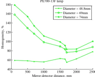
An important characteristic of the spatial distribution is its homogeneity (Eq 1). Where IMAX, IMIN, IAVG correspond to the maximal, minimal and average (over

circle) values of the flux density. Figure 11 represents the variation of the homogeneity as a function of the mirror-baffle distance for different diameters.

AVG MIN MAX I I I Homog  (Eq. 1) It is logical that the homogeneity becomes smaller for smaller diameters. Similar results were observed for other lamps. Figure 12 summarizes the results for all studied lamps with a fixed diameter of 47,4 mm.

Figure 11: The homogeneity as function of mirror-baffle distance for PE700-13F lamp.

Figure 12: The homogeneity as function of mirror-baffle distance for all studied lamps.

0 500 1000 1500 2000 2500 0 10 20 30 40 50 60 Mirror-detector distance, mm AVG flux density, kW/m 2 PE700-13F lamp Diameter = 48.8mm Diameter = 69mm Diameter = 74mm 0 500 1000 1500 2000 2500 0 10 20 30 40 50 60 Mirror-detector distance, mm AVG Flux density, kW/m 2 PE300-13F PE500-13F PE700-13F PE1000-13F PE1200-13F 0 500 1000 1500 2000 2500 40 60 80 100 120 140 160 180 Mirror-detector distance, mm Homog ene ity, % PE700-13F lamp Diameter = 48.8mm Diameter = 69mm Diameter = 74mm 0 500 1000 1500 2000 2500 40 45 50 55 60 65 70 75 80 85 Mirror-detector distance, mm Homog ene ity, % at 47.4mm diameter PE300-13F PE500-13F PE700-13F PE1000-13F PE1200-13F

3. OPTICAL TESTS FOR VALIDATION OF THE DESIGN

Experimental validation of the optical design includes measurement of the flux divergence, of the power density produced by the illumination system and evaluation of the deviation from the real solar conditions.

3.1. Experimental measurement of the angular distribution

Concerning the divergence achieved by the illumination setup, there is an upper bound due to the geometric configuration, as shown by figure 13 where M1 is the collimating mirror with a radius of 38 mm; 𝛿_𝑚𝑎𝑥 is the maximum divergence half angle; 23.7 mm and 26.7 mm are the inside and outside radii of the entrance pupil. Figure 14 shows the maximum divergence half angle 𝛿𝑚𝑎𝑥 as a function of the distance between M1 and the area of interest (entrance pupil). All three lines show similar behavior: the further the pupil is from the mirror, the lower is the maximum divergence. The two solid lines correspond to the geometrical limits of the set up and the dot line corresponds to the average radius on the mirror. This choice was taken after an observation of the spatial profile of the illumination on the mirror (figure 15). This profile is non-uniform, presenting a donut-shape with a depletion zone in the center due to the spider of the lamp, and a maximum around r/2. Most of the rays falling inside the pupil come from this zone, therefore reducing the average divergence.

Figure 13: The definition of the maximal angular divergence.

Figure 14: The maximum divergence half angle 𝛿𝑚𝑎𝑥 as function

of the distance.

Figure 15: The spatial profile on the mirror.

The method to measure the divergence was to use an array of pinholes located in the area of interest with a screen located at a given distance from the pinholes. The size increase of the pinholes image on the screen is related to the divergence of the incident beam. The purpose of having an array of pinholes (instead of one pinhole) is twofold: first to

1 1.5 2 2.5 3 3.5 4 0.5 1 1.5 2 2.5 3 3.5 4 distance [m] M a x im u m h a lf d iv e rg e n c e [ d e g ]

inside illumated area on coronna diam 53.4mm inside baffle through pupil 47.4mm

rays coming from average radius 20mm on mirror

Mirror 38mm 23.7mm inside pupil 26.7mm outside pupil Area of interest 𝛿_𝑚𝑎𝑥

r

have multiple values to decrease the error and second to assess the potential distribution of divergence over the area of interest.

Figure 16 shows the divergence measurement principle and shows a zoom on the definition of the first D1 and second D2

measured diameters. There, the red dot line defines the location of the pinholes array and the green line defines the screen, a sheet of paper in this case. The half divergence angle 𝛿 can be derived as:

𝛿 = atan 𝐷2−𝐷1

2𝑑 (Eq.2)

Figure 16: Experimental schema of the divergent measurement (left) and zoom on the diameters definition (right).

Two tests were performed with two different pinhole arrays (figure 17): 3x3 array with 10 mm Ø pinholes and 7x7 array with 3.2 mm Ø pinholes. This figure shows the image of the pinholes and screen behind (a) and the images of the spots on the screen from 10 mm (b) and 3.2 mm (c) Ø pinholes.

a) b) c)

Figure 17: Images of a) pinholes arrays and screen; b) spots on the screen from 3x3 pinhole arrays; c) spots on the screen from 7x7 pinhole arrays.

Top pictures of figures 18 and 19 were processed with MATLAB. Graphs 18 and 19 show the processed pictures of the 3.2 mm Ø pinholes at a distance of 1500 mm from the mirror; the screen being 50 mm and 100 mm behind the pinholes, respectively. The diameter of the central spot is approximately 6.2mm (diameter at 10%) leading to a half divergence around 1.7 deg. It is important to note that the accuracy of the method is limited and driven by the uncertainty on the second diameter measurement and the distance between the pinholes and the screen. Indeed, the image of the pinhole is not sharp and the diameter of the spot is blurred due to the penumbra.

𝐷2 penumbra 𝐷₁ 𝑑 M1 𝐷₂ array of pinholes 𝐷₁ 𝑑 screen

Figure 18: MATLAB result for 7x7 arrays with 3.2mm Ø pinholes with the screen at 50 mm behind.

Figure 19: MATLAB result for 7x7 arrays with 3.2mm Ø pinholes with the screen at 100 mm behind.

Assuming following uncertainties:

- Uncertainty on the distance between the screen and the pinholes array: +/-2 mm,

- Uncertainty on the measurement of the spot size (camera distortion, blurred diameter, uncertainty on the pinhole size): +/- 1 mm.

𝛿 = atan (6.2−3.2)±1_{2× 50±2} = 1.7+0.7−0.6_{deg (Eq.3)}

The same calculation can be done with the central spot for the image with screen position at 100 mm behind the pinholes (figure 19):

𝛿 = atan (8−3.2)±1

2× 100±2 = 1.4 +0.3

−0.3_{deg (Eq.4)}

These angular divergence results correspond to the predictions of the simulations performed with the ASAP raytracing software (i.e. <2 deg) and in-flight condition for the EUI instrument.

3.2 Experimental measurements of the spatial distribution

Finally, the experimental validation of the optical design was completed by the measurement of the irradiance spatial distribution. Two measurement methods were used and compared. The first one consists in the illumination intensity

measurement using a pyranometer and a neutral density filter and the second one uses photodiodes to map the flux distribution.

3.2.1 Measurement by pyranometer

The pyranometer CMP21 was used to measure the intensity at several distances from the mirror. A neutral density reflective filter OD1 (density 1.0  0.1 attenuation factor) is used to protect the pyranometer which is limited to 4 kW/m². Figure 20 shows the measurement points with the pyranometer from which a trend curve is extrapolated. A scaling factor is applied depending on the measured source (ratio of the visible output in datasheet: 21000 Lumens for PE700C-13F, 23500 for the PE100D-13F and 40000 for the PE1500D-13F). The scaling could also be done on the radiant output.

Figure 20: Result of intensity measurement by pyranometer.

To measure the uniformity, a white screen was first used of which pictures were taken. The pyranometer was then used to measure the intensity at the same location (the measured intensity is the average on the active area of the pyranometer, i.e. a 25mm Ø circle). Figure 21 shows an example of the picture of the screen. The picture is then processed with MATLAB and a profile of the spatial uniformity can be derived, as shown in figure 22. It must be noted that the camera used to take the pictures slightly saturated in the center. This effect can be observed by noticing that the center pixels are white, which gives a flattening of the Gaussian profile top part.

The resulting MATLAB irradiance profile is centered and approximated by a Gaussian curve. The dimensionless profiles are then scaled so that their average over a 25 mm Ø disc matches the pyranometer measured values at different distances. The measured intensity on the pyranometer over the 25 mm active diameter at 1225 mm mirror - detector distance is 26 kW/m2. 1 1.5 2 2.5 0 5 10 15 20 25 30 35 40

distance from mirror [m]

In te n s it y o n p y ra n o m e te r s u rf a c e ( 2 5 m m d ia m ) [k W /m

²] Measurements Cermax PE700C-13F

Extrapolation Cermax PE700C-13F scaling for Cermax PE1000D-13F scaling for Cermax PE1500D-13F

Figure 21: Image of intensity distribution on the screen at 1225 mm distance from mirror.

Figure 22: Result of MATLAB analyzes for spatial uniformity.

3.2.1 Measurement by photodiode

The measurement of the intensity distribution with the photodiodes was performed at a distance of about 1 m from the mirror. The detectors were centered on the optical axis of the mirror and were placed on a translation table. Moreover, the aluminum pinhole with a 1 mm diameter was placed before the detector, giving the mapping of the distribution (figure 23).

a) b) c)

Figure 23: a) Image of the Cermax lamp and collimating mirror; b) Image of the detector profile fixed on the lever; c) Image of the aluminum pinhole.

The measurements were performed with 5 mm steps and covered an area of 40x40 mm. Figure 24 shows the results of the measurements with low power photodiodes 818UV used in combination with neutral density filter OD2.

Figure 24: Measured power density with low power 818UV photodiode.

The average intensity over 40 mm Ø at 1000 mm from the mirror is about 35 kW/m2, that corresponds to the simulation data of ASAP (figure 9) and the extrapolated values from the pyranometer (figure 20). The estimated homogeneity over a diameter of 40 mm is about 128 % which is worse than the predicted value from ASAP of about 60 %.

Similar results were obtained with high power detectors 818P-20-12 (figure 25).

Figure 25: Measured power density with high power detector 818P-20-12 photodiode.

39.3 38 36.5 35 33.5 0 10 20 30 40 50 -2,5 -2 -1,5 -1 -0,5 0 0,5 1 _{1,5 2} 2,5 Vertical displacement, cm Power de nsi ty, kW/ m 2 Horizontal displacement, cm 50-57 40-50 30-40 20-30 10-20 0-10 39.5 38 36.5 35 33.5 0,0 10,0 20,0 30,0 40,0 50,0 1 _{2 3} 4 _{5 6} 7 _{8 9} 10 11 Vertical displacement, cm Po wer den sit y, kW /m 2 Horizontal displacement, cm 0,0-10,0 10,0-20,0 20,0-30,0 30,0-40,0 40,0-50,0

4. THERMAL BALANCE TEST

The thermal balance test set-up is composed of the illumination setup, the 2 meters diameter FOCAL2 vacuum chamber of CSL, a thermal shroud simulating the S/C cavity radiative environment along with a dedicated panel for the different conductive thermal interfaces, three equivalent feedthroughs and the EUI instrument (figure 26).

Figure 26: Setup overview with the illumination setup outside the chamber on the left and the instrument upside-down inside the thermal shroud.

4.1 How to simulate the Sun input

The 13 solar constants (17.5kW/m²) solar irradiance is provided by three Cermax Xe lamps located outside the vacuum chamber, each one dedicated to one EUI channel (figure 27). Calibration of the intensity and mapping of the uniformity of the incoming solar flux was carried out. The intensity was measured with pyranometer CMP21 used in combination with neutral density filters. The uniformity was assessed by mapping the solar flux with a photodiode.

Figure 27: Top left: the CERMAX lamp; bottom left: the pyranometer; right: the illumination set-up

The irradiance measurement was performed as follows:

Once the lamps are aligned, the pyranometer is used to measure the intensity at the center (giving the average over its 25mm Ø active area). A rough relative mapping of the total illuminated area is performed using the photodiode. A picture is taken of a ruled sheet of paper. A finer relative mapping is extracted from the picture and compared to the photodiode mapping. If the relative mappings match, the fine mapping is scaled using the average value given

Centre Spatial de Liege FOCAL2 Vacuum chamber

Vacuum chamber flange

Illumination set-up located outside the vacuum chamber

Copper thermal shrouds simulating the S/C cavity radiative environment

Support of the thermal shrouds

EUI instrument inside the thermal shrouds Copper pipes simulating the

feedthroughs of the S/C inside the heat shield

CERMAX lamp

CMP21 pyranometer Vacuum chamber flange

Vacuum chamber optical apertures

CERMAX lamps

by the pyranometer over its active area. Figure 28 shows the raw picture and the scaled mapping of the HRIEUV

irradiance. Table 4 summarizes the mapping results for the three channels.

Figure 28: Mapping of the HRIEUV irradiance. Right: raw picture with arbitrary units, left: processed picture in [kW/m²]

HRIEUV HRILya FSI

qS average [kW/m²] 16.6 17.6 16.3

max deviation [%] 15 6 16

min deviation [%] -17 -15 -17

Table 4: Measured irradiance and maximum/minimum deviation from average value at the three channels of EUI instrument

4.2 How to simulate the spacecraft thermal environment

A dedicated thermal panel is placed between the instrument and its rotating support to simulate the conductive environment of the feet and the radiative environment below EUI.

The different conductive thermal interfaces are made of copper straps connected to a common panel (interface panel). This panel is cooled down with LN2. Each interface temperature is regulated (PWM) through heaters onto each strap. Each heater duty cycle is recorded to give information about the heat load on the corresponding interface.

The IR load coming from the spacecraft feedthroughs is simulated by copper pipes heated up with custom ceramic heaters in addition to the lamps. Figure 29 shows the copper pipes with the ceramic custom heater (in white).

Figure 29: Setup feedthrough with custom ceramic heater

The six copper shrouds of the thermal tent simulate the 50°C radiative thermal environment of the spacecraft.

Copper pipes simulating the S/C feedthroughs through the heatshield

Copper shroud

Mounting structure for the shrouds and the

instrument Copper pipes simulating

the S/C feedthroughs through the heatshield Custom ceramic heaters

4.3 Results of the thermal balance

A mapping of the flux was made just before chamber closing to check the homogeneity and the irradiance. The irradiance was measured with the pyranometer and the mapping was made with a photodiode.

The results are presented on figure 30:

Figure 30: Mapping of the thermal balance Sun flux

The irradiance is measured with the pyranometer (figure 31). It is mounted on a dedicated structure inside the chamber, at the location of the EUI entrance, in front of an optical density filter.

Figure 31: Mapping of the thermal balance Sun flux: experimental set-up (left). Right: illumination set-up, ouside the

chamber, functionning

The pyranometer indicated an irradiance of 18182 W/m2 at the level of EUI entrance.

5. CONCLUSIONS

We could observe that the experimental results and studies were in line with the results obtained during the thermal balance. The different laboratory experiments (measurements of the flux, the homogeneity and the divergence)

performed during the 2012 year were fruitful and lead to a successful thermal balance test end of 2013 and beginning of 2014 of the EUI instrument.

6. ACKNOWLEDGEMENTS

The EUI instrument is developed in a collaboration which includes the Centre Spatial de Liège and Royal Observatory of Belgium (Belgium), the Institut d’Astrophysique and Institut d’Optique (France), the UCL Mullard Space Science Laboratory (UK), and Max Planck Institute for Solar System Research (Germany).

The Belgian institutions are funded by Belgian Federal Science Policy Office; the French institutions by Centre National d'Etudes Spatiales (CNES), the UK institution by the UK Space Agency (UKSA); and the German institution by Deutsche Zentrum für Luft- und Raumfahrt e.V. (DLR).

The CMOSIS Company, located in Antwerpen, Belgium, is responsible of the detector development; under the ESA-PRODEX contract no. 4000110352.

7. REFERENCES

[1] Halain J.-P., Rochus P., Renotte E., Appourchaux T., Berghmans D., Harra L., Schühle U., Schmutz W., Auchère, F., Zhukov A., Dumesnil C., Kennedy, T., Mercier R., Pfiffner D., Rossi L., Tandy J., Smith P., “The EUI instrument on board the Solar Orbiter mission: from breadboard and prototypes to instrument model validation” Proc. SPIE 8443, (2012)

[2] Cermax lamps engineering guide. ILC Technology, Inc.1998

[3] Cermax products and specifications, short arc, xenon lamps, modules. Perkin Elmer, 2006