HAL Id: hal-00566284
https://hal-brgm.archives-ouvertes.fr/hal-00566284v2
Submitted on 15 Feb 2011
HAL is a multi-disciplinary open access
archive for the deposit and dissemination of
sci-entific research documents, whether they are
pub-lished or not. The documents may come from
teaching and research institutions in France or
abroad, or from public or private research centers.
L’archive ouverte pluridisciplinaire HAL, est
destinée au dépôt et à la diffusion de documents
scientifiques de niveau recherche, publiés ou non,
émanant des établissements d’enseignement et de
recherche français ou étrangers, des laboratoires
publics ou privés.
Hydraulic and thermal impact modelling at the scale of
the geothermal heating doublet in the Paris Basin,
France
Morgane Le Brun, Virginie Hamm, Simon Lopez, Pierre Ungemach, Miklos
Antics, Jean Yves Ausseur, Elisabeth Cordier, Elodie Giuglaris, Patrick
Goblet, Pierre Lalos
To cite this version:
Morgane Le Brun, Virginie Hamm, Simon Lopez, Pierre Ungemach, Miklos Antics, et al.. Hydraulic
and thermal impact modelling at the scale of the geothermal heating doublet in the Paris Basin,
France. 36th Stanford Geothermal Workshop, Jan 2011, Stanford, United States. pp.403-416.
�hal-00566284v2�
PROCEEDINGS, Thirty-Sixth Workshop on Geothermal Reservoir Engineering Stanford University, Stanford, California, January 31 - February 2, 2011 SGP-TR-191
HYDRAULIC AND THERMAL IMPACT MODELLING AT THE SCALE OF THE
GEOTHERMAL HEATING DOUBLET IN THE PARIS BASIN, FRANCE.
M.Le Brun1*, V.Hamm1, S.Lopez1, P.Ungemach2, M.Antics2, JY.Ausseur4, E.Cordier3, E.Giuglaris5, P.Goblet3, P.Lalos2
BRGM
3, avenue Claude Guillemin Orléans, 45000, France e-mail: m.lebrun@brgm.fr
ABSTRACT
The Paris Basin is extensively developed for the geothermal district heating (GDH) of approximately 150 000 dwellings. As of late 2010, thirty four GDH systems apply the doublet concept in the Paris suburban area and mine the heat of the Dogger reservoir, a limestone formation of Mid-Jurassic age at depths ranging from 1500 to 2000 m. As the brine is fully reinjected, cold water bodies progressively invade the reservoir around injector wells inducing both thermal and hydraulic interactions at the doublet scale.
The premature production well cooling and the sustainable development of the resource highlight two critical parameters, the thermal breakthrough time (tB) and the extent of the cooled fluid bubble(S) respectively.
First, a set of benchtest simulations was launched to compare the sensitivities of tB and S parameters to selected reservoir conceptual model typologies. These simulations were applied on a GDH doublet undergoing a suspected thermal breakthrough. Five reservoir modelling teams validated their “in house” simulations by (i) checking an analytical (Gringarten-Sauty, 1979) solution, and (ii) testing three candidate reservoir structures on the doublet considered remotely located (i.e. not interfering with nearby exploitations) for a first step. The outcome resulted in a rewarding insight into the variability of simulation outputs. An additional segment will enable the actors to compare their modelling expertise on the same doublet considered in interaction with the other GDH operations located in its environment.
Second, BRGM carried out a survey towards various rehabilitation schemes (a new doublet or a triplet) and their contribution toward sustainability standards. From a hypothetical, twenty five year life, doublet
simulation, an initial hydraulic/temperature field was derived.
Then, several new well locations were simulated and isotherms, alongside production well cooling kinetics, compared accordingly. A two-stage rehabilitation scheme, i.e. triplet then a new doublet, seems to reconcile the resource longevity and the economic demand. Further work is required to compare the different designs with a method integrating both the impact of the geothermal exploitation on the resource and the lifetime of the exploitation in a single mathematical factor.
THE GEOTHERMAL EXPLOITATION IN THE PARIS BASIN
Historical perspective
Geothermal development in the Paris Basin started in the early 1970s with the main target being the Dogger aquifer. Nearly all operations use the “doublet” technology consisting of a closed loop with one production well and one injection well.
Of the 55 doublet systems that have been implemented, most of these in the 1980s, 34 are still in operation, mainly in the Val de Marne and Seine St Denis area. (Lopez et al., 2010). With the current geothermal revival of the Paris Basin, the exploitation of the resource of the Dogger aquifer is facing new challenges (Hamm et al., 2009)
Issues linked to the doublet technology
Injection of the cooled brines creates a cold water body at the injection well and the resource has been cooled by the 30 years of reinjection.
The thermal breakthrough (Tb) is expected to occur in the coming years, inducing the decrease of the
production wells temperature (represented by the final production well temperature Tf) and as well as the recovered energy.
Most of the wells still operating are next to 30 years old. They would need to be restored or shut down for scaling and/or corrosion problems, implying the drilling of new ones. The rehabilitation scheme has to take into account the area (S) mined by the first doublet.
Management and the modelling tool
Modelling has been used for around 20 years to forecast the lifetime of operations and the impact of the development of new operations in the Dogger aquifer in the Paris Basin (Lopez et al., 2010). One of the key points in the modelling process is the conceptual model of the reservoir. To evaluate the influence of the conceptual model on the extent of the cold water body and the production well temperature, 1 group of 5 teams of modellers coming from different organisations (university, private structures, public structure) has been created. This article presents the results of its work on the sensitivity of the modelling results (tb and S) to the reservoir conceptual model.
As the geothermal wells are getting older, the question of the schemes of rehabilitation is more and more sensitive. The BRGM carried out a study on a isolated doublet to evaluate the impacts of different rehabilitation schemes on the lifetime of the new exploitation (Tb) and the resource (S).
IMPACTS OF THE STRUCTURE OF THE CONCEPTUAL MODEL ON THE NUMERICAL RESULTS
Five teams participate to the benchmark with specific modelling software and an “in-house” method summarised in the following table.
Table 1: Definition of the modelling teams
Group Software Numerical scheme
CFG (Comsol-1) Comsol Finite element
GPC-IP (Tough2-2) Tough2 Finite difference
Antea (Marthe-3) Marthe Finite volume
Mines ParisTech
(Metis-4) Metis Finite element
BRGM (Marthe-5) Marthe Finite volume
The numbers attached to the software names in the group column correspond to the team number. The benchmark is cut into two parts, the first one checking the ability of the modelling software to reproduce an analytical solution (tb and Tf), the second part comparing the results (tb, Tf and S) of simulations based on different conceptual models.
The doublet of Alfortville is chosen as the reference doublet of the benchmark. The production well is called GAL2 and the injection well GAL1.
From this doublet is derived the structure of the reservoir and the exploitation sequence (timing of the different flowrates of water injected and produced, temperature injected)
Comparison between an analytical solution and the model results
Principle
The 1D analytical solution of Gringarten and Sauty is used to calculate the temperature at the production well Tw(t).
⎟⎟
⎠
⎞
⎜⎜
⎝
⎛
⎪
⎪
⎭
⎪
⎪
⎬
⎫
⎪
⎪
⎩
⎪
⎪
⎨
⎧
⎥
⎦
⎤
⎢
⎣
⎡
⎟⎟
⎠
⎞
⎜⎜
⎝
⎛
−
∗
=
−
−
∫
−Q
d
Q
d
D
S
d
t
Q
d
D
S
d
erfc
T
T
t
T
T
d i wψ
ψ
λ
ψ
2 / 1 max max 0 0)
/
(
²)
/
(
)
/
(
²)
/
(
)
(
Equation 1: Gringarten&Sauty equation
λ
an adimensional parameter qualifying the heat exchange between the reservoir and the walls tD the reduced time are defined by the following equations:⎟
⎠
⎞
⎜
⎝
⎛
⎟⎟
⎠
⎞
⎜⎜
⎝
⎛
=
⎟
⎠
⎞
⎜
⎝
⎛
⎟⎟
⎠
⎞
⎜⎜
⎝
⎛
=
²
²
hD
Qt
C
C
t
D
Qh
C
K
C
C
A A w w D R R R A A w wρ
ρ
ρ
ρ
ρ
λ
Equation 2: definition of the adimensional parameters for the walls of the reservoir and the reduced time.
The aquifer heat capacity is calculated with the following equation: R R w w A A
C
θρ
C
θ
ρ
C
ρ
=
+
(
1
−
)
Equation 3: definition of the aquifer heat capacity Each team checks if its modelling tool can reproduce this analytical solution with the following hypothesis:
• The fluid is considered as pure water, viscosity and the fluid density are constant. • The aquifer is considered as a one layer
aquifer, with a 9m thick (h) productive layer, with an infinite horizontal extension. Two impervious layers are located at the top and the bottom of the productive layer • The transmissivity of the aquifer is 5D, the
porosity
θ
is 17%. The thermal2.5 W/m/K and 0.6 W/m/K respectively. The thermal conductivity is neglected in the aquifer in the flow direction. The heat capacity of rock (
ρ
RC
R) and water (ρ
wC
w) are 2.16 MJ/m3/K and 4.18 MJ/m3/K respectively• The heat transport is convective in the aquifer and conductive in the vertical direction in the impervious layers. • Initially, temperature is homogeneous
between rock and water and the impervious layers are in thermal equilibrium with the aquifer at T0=75°C. During the injection, the equilibrium between rock and water is instantaneous.
• The dispersivity should be neglected but a minimal value for this dispersivity is accepted for ease of converging for the models
• The flowrate of injection and production is constant over 30 years at Q=193 m3/h. The injection temperature is also constant at Ti=49°C.
• The production and the injection well are separated from D=1130m from each other.
Results
Two parameters are compared between the analytical solution and the model solution: the final temperature at the production well (ΔTf), the thermal
breakthrough time (Δtb). The thermal breakthrough is defined as the time when the first sign of temperature decreasing appears, that is when the production temperature reaches 74.9 °C. The final production well temperature corresponds to the temperature at 30 years of simulation. The results are presented in the following table
Table2: Synthesis of the comparison between the simulation and the analytical results
Team Model tb (year) model Tf (°C) Δtb (year) ΔTf (°C) Comsol-1 6 70.8 0 0 Tough2-2 6 71.6 0 0.8 Marthe-3 4 69.4 2 1.4 Metis-4 6 70.8 0 0 Marthe-5 4 70.8 2 0
The Tough2-2 simulation gives a final production temperature above the analytical solution, due to the variation of viscosity that has been included in the Tough2 software.
The Marthe-3 simulation under estimates the final temperature compare to the Marthe-5 simulation. A finer vertical discretisation in the Marthe-5
simulation gives a better approximation of the heat transfers between the walls and the reservoir. Nevertheless, the thermal breakthrough of the Marthe-3 and -5 simulations occurs earlier than the analytical solution, due to the calculation of the equivalent vertical conductivity that underestimates the heat transfers between the walls and the reservoir. The Comsol-1 and Metis-4 simulations forecast the same temperature variation, and hence the same final temperature as the analytical solution, which means the physical representation of the reservoir is close to that of the analytical solution and the thermal role of the walls is correctly taken into account.
The following graphic displays the different production temperature curves which bound the analytical solution. The Marthe-5 meanT curve displays the evolution of the temperature on the whole thickness of the reservoir, whereas the Marthe-5 curve represents the temperature in the first layer just below the wall.
68 69 70 71 72 73 74 75 76 0.00 5.00 10.00 15.00 20.00 25.00 30.00 years pr od uc ti o n t em p er at ur e ( °C ) Analytical solution (Gringarten&Sauty) Marthe_3 Metis Marthe_5 Marthe_5 meanT Comsol_1 Tough2_2
Comparison between the thermal and hydraulic results with regards to the conceptual model
Principle
The exploitation sequence is common as indicated in the following table.
Table 3: Production and injection sequence for the 30 years of simulation Flowrate (m3/h) Injection temperature (°C) Winter (8 months) 231 44 Summer (4 months) 93 60
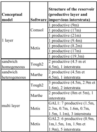
The different conceptual models tested are based on the flowmeters of GAL1 and GAL2 and vary the number and the thickness of the productive layers and impervious interstrata in the reservoir. Three types of conceptual models are tested as described in the following table.
Table 4: The one-layer, multi-layer and sandwich conceptual models along with their sub models (each one has a particular structure
Conceptual
model Software
Structure of the reservoir (productive layer and impervious interstrata) 1 productive (9m) 1 productive (17m) 1 productive (21m) 1 productive (9.4m) 1 productive (8.2m) 1 productive (17m) 1 productive (19.3m) sandwich homogeneous Tough2 2 productive (4.5 m et 4.5m), 1 interstrata sandwich heterogeneous Marthe 2 productive (4.5m et 4.5m), 1 interstrata Tough2 3 productive (4.5m, 2.9m et 1.6m), 2 interstrata Marthe 2 productive (8m et 5m), 1 interstrata Metis GAL1: 7 productive (1.5m, 2.3m, 0.7m, 1.6m, 0.7m, 1.5m, 1.1m), 3 interstrata Metis GAL2: 6 productive (0.9m, 1m,1.5m, 1m, 1.9m et 1.9m), 5 interstrata 1 layer Comsol Metis multi layer
The output of each model are the production well temperatures over the 30 years of simulation and the characteristic dimensions of the cooled water body at 5 years, 10, years, 20 years and 30 years of simulation as shown on the figure below.
Figure 2: Characteristic dimensions of the 72°C isotherm
Construction of the different conceptual model
Two ways of construction are used for the one layer model:
• Based on one flowmeter, the productive layers are put together and their thickness is summed into one layer.
• The top of the upper productive layer and the bottom of the lowest productive layer delineate the model layer.
The interstrata which act as a thermal buffer are not considered
Two types of multilayer model are studied:
• The productive layers on a flowmeter are gathered into 3 or 2 productive layers according to their contribution to the total flowrate. They are separated by impervious interstrata (Tough2 and Marthe)
• Each productive layer appearing on the flowmeter is represented in the model with the same location and thickness (Metis) The construction of the sandwich conceptual model follows several steps as first described by GPC-IP (Ungemach et al, 2009):
• the productive layers are cumulated together into one global productive layer
• the impervious interstrata layers acting as a storage of heat are cumulated into one buffer layer
• the global productive layer is split into two symmetric parts by this buffer zone
The homogeneous sandwich model is a tabular model. For the heterogeneous sandwich model, the horizontal structure is interpolated between wells in order to account for lateral variability.
Results
The evolution of the production temperature is compared for each type of conceptual model and then between the three types of conceptual model.
In the comparison tables, the range of values for the thermal breakthrough time and the final production temperature is given in the tb and Tf columns.
• For the one layer conceptual models, the variation Δtb for tb is 5 years and 1.5°C for ΔTf as shown on the table 5.
Table 5: ranges for tb and Tf for the one layer conceptual model
Conceptual
model Curve Structure
tb (years) Tf (°C) Comsol-1 9m 1 productive (9m) Metis-4 9.4m 1 productive (9.4m) Metis-4 8.2m 1 productive (8.2m) Metis-4 17m 1 productive (17m) Metis-4 19.3m 1 productive (19.3m) 1 layer 6.5 to 11.5 70 to 71.5
The bottom curve is the 8.2m model and the top curve is the 19.3m model as shown on the graphic 2. The thinner the section for the waterflow, the earlier the thermal breakthrough occurs. These results confirm that the model only based on the thickness of the productive layers is the most pessimistic model in terms of tb and Tf.
The 9m layer model is studied by two simulations (Metis-4 and Comsol-1). The thermal breakthrough occurs approximately at the same time but production temperature is decreasing slowlier in the model Comsol-1 inducing a Tf greater by 1°C. This difference is not fully understood, it may come from the way the thermal dispersivity is taken into account in the model.
The curve of the Metis-4 9.4m simulation lays under the analytical solution at the end of the simulation. As the thermal conduction in the reservoir is included in the model solution, the final temperature production is supposed to be lower with this solution than for the analytical one.
d D
70.0 71.0 72.0 73.0 74.0 75.0 76.0 0 5 10 15 20 25 30 35 years pr oduct io n t em p erature ( °C) Metis_4 9.4m Metis_4 17m gringarten Metis_4 8.2m Metis_4 19.3m Comsol_1 9m
Figure 3: Variability of the production temperature curves for the one layer conceptual model • For the multi layer conceptual model, Δtb is
1 year and ΔTf is 3.5°C as shown on the table 6.
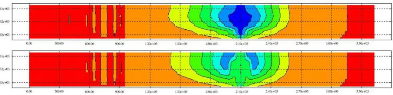
Despite the thermal breakthrough is relatively equivalent for each simulation, the range for the final production temperature is wider. The slope of the temperature curve gets smaller with the number of layers in the model. The results of the multi layer models seem very dependent of the layering of the reservoir, especially when some layers are more hydraulically conductive than others. Vertical
temperature cross-sections in the Metis-4 GAL1 and GAL2 simulations (Figure 3) show the high conductive layers being rapidly warmed by the interstrata during the low flowrate and higher injection temperature period. That phenomenon slows down the cooled body progression. Other Metis-4 GAL1 and GAL2 simulations demonstrate this phenomenon doesn’t occur with a constant Q and
Tinj sequence.
Table 6: ranges for tb and Tf for the multi layer conceptual model Conceptual
model Curve Structure
tb (years) Tf (°C) Tough2-2 3 productive Marthe-5 2 productive Metis-4 GAL1 7 productive Metis-4 GAL2 6 productive multi layer 8 to 9 71 to 74.5
Figure 4: Heating of the GAL2 reservoir between the end of the winter period (top figure) and the end of the summer period (bottom figure)
71 71.5 72 72.5 73 73.5 74 74.5 75 75.5 0 5 10 15 20 25 30 35 years pr oduction tempe ra ture (°C ) Tough2_2 marthe_3 metis_4 GAL1 metis_4 GAL2
Figure 5: Variability of the results for the multi layer model
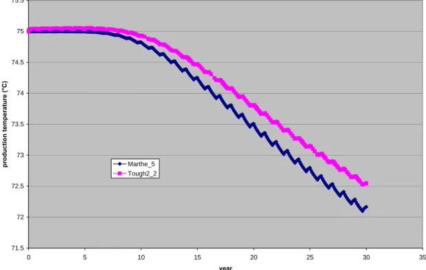
• For the sandwich conceptual model, the tb variation is 2 years and the Tf variation is 0.5 °C as shown on the following table.
The homogeneous model is optimist with the tb occurring at 10 years. In the heterogeneous model, some layers have a higher transmissivity and may allow the cooled front to arrive faster than in the
homogeneous model.
Table 7: ranges for tb and Tf for the sandwich conceptual model
Conceptual
model Curve Structure
tb (years)
Tf (°C) sandwich
homogeneous Tough2-2 2 productive sandwich
heterogeneous Marthe-5 2 productive
8 to 10 72 to 72.5
71.5 72 72.5 73 73.5 74 74.5 75 75.5 0 5 10 15 20 25 30 35 year pr oduction temper atur e (° C) Marthe_5 Tough2_2
Figure 6: Variability of the results for the sandwich model
• Comparing the three types of conceptual model (table 7), the one layer model seems the most sensitive for tb and the multi layer model the most sensitive for the final production temperature. The sandwich model seems to be a good trade off between tb and Tf.
Table 8: Comparison of the variability of the results between the three types of conceptual model
Conceptual model Δtb (years) ΔTf (°C)
one layer 5 1.5
multi layer 1 3.5
sandwich 2 0.5
Looking at the graphic 5, the range of the simulation results is 5 years for tb and 4.5°C for Tf. This variability of the simulation results is higher than expected from different conceptual models derived from 1 case study.
The different conceptual models are gathered into three families according to the shape of the curves:
1- The one layer model taking into account only the productive layers (Metis 9.4m and 8.2m). The buffer role of the interstrata is neglected.
2- The sandwich models (marthe and tough2), the one layer models whose thickness includes the interstrata (metis 17m and
19.3m) and the coarse multilayered models (Tough multilayer, marthe multilayer). The buffer role of the interstrata is thermally represented in the sandwich and multilayer models (heat transfer between the impervious interstrata and the aquifer slows the progression of the thermal front) and hydraulically represented in the one layer models (the thicker productive layer induces a slower velocity of the cooled particles). 3- The multi layer models representing the
layering of the flowmeters (metis Gal1 and Gal2). These finely layered models propagate the wells information at the doublet scale, the heat exchange surface is maximum between the productive layers and the interstrata. The decreasing in temperature is thus much slower than for the other models.
Given this wide range of results, another set of simulations were launched with a mean flowrate and temperature injection sequence for each of the models. The results are similar to the variable sequences for first and second family but the results for the third family are similar to the second family. It seems the variability of the results for the finely layered models is also linked to the exploitation sequence.
70 70.5 71 71.5 72 72.5 73 73.5 74 74.5 75 75.5 0 5 10 15 20 25 30 years pr odu ct io n t em p er at ur e ( °C) Tough2_2 multilayer marthe_5 sandwich Comsol_1 one layer 9m Tough2_2 sandwich Metis_4 multilayer GAL1 Metis_4 multilayer GAL2 Metis_4 one layer 9.4m Metis_4 one layer 17m Metis_4 one layer 8.2m Metis_4 one layer 9.3m Marthe_3 multilayer
Figure 7: sensitivity of the results for the three types of models
• The last output of the simulation is the dimension of the cooled water body. The
characteristic dimensions are summarised in the following tables.
Table 9: longitudinal extension of the cooled water body for the different conceptual models
5 years 10 years 20 years 30 years 5 years 10 years 20 years 30 years 1 productive (9m) 1040 1414 1816 1903 1 productive (17m) 855 1167 1724 1840 1 productive (21m) 790 1077 1551 1813 1 productive (9.4m) 1597 1706 1811 1900 1 productive (8.2m) 1611 1711 1831 1909 1 productive (17m) 1537 1647 1776 1850 1 productive (19.3m) 1525 1633 1749 1833 homogeneous 990 1313 1763 1862 heterogeneous 1010 1360 1780 1870 3 productive 1052 1408 1768 1842 2 productive 1015 1435 1790 1875 7 productive 1556 1624 1672 1688 6 productvie 1564 1626 1660 1670 Conceptual model 1 layer multi layer sandwich 1175 1772 1866 1297 1523 1723 1769 1279
D (lengthwise extension in m) Mean D (m)
1479 1751 1864
Table 10: lateral dimension of the cooled water body 5 years 10 years 20 years 30 years 5 years 10 years 20 years 30 years 1 productive (9m) 960 1192 1440 1606 1 productive (17m) 806 1030 1324 1484 1 productive (21m) 760 976 1256 1462 1 productive (9.4m) 996 1238 1480 1638 1 productive (8.2m) 1012 1245 1493 1649 1 productive (17m) 867 1107 1370 1547 1 productive (19.3m) 829 1064 1344 1504 homogeneous 911 1127 1387 1554 heterogeneous 900 1100 1340 1480 3 productive 959 1179 1395 1519 2 productive 920 1180 1450 1620 7 productive 917 1056 1153 1190 6 productive 939 1056 1128 1128 934 1118 1282 1 layer multi layer Conceptual model 1387 1556 906 1114 1364 1517 1371 sandwich
d (transverse extension in m) Mean d (m)
890 1122
The means of the characteristic dimensions over the simulation time are in the same range of value for the different models. They increase rapidly during the first 20 years and then the rate of progression diminishes.
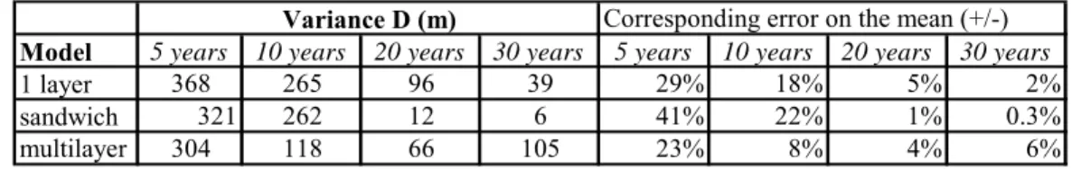
The table 9 below calculates the representative deviation for 1 type of conceptual model for the 4 output times. This deviation corresponds to the error in percentage on the mean and represents the variability of the results. Thus a decreasing error means the dispersion of the different values tend to decrease.
For the longitudinal length, the error decreases with time for all the models. For the lateral length, the error decreases are stabilizes except in the case of the multilayer model where it increases. This
characteristic length is more sensitive to the layering of the model than the longitudinal one because of the strong influence of the production well in the lengthwise direction. As for the temperature curve for the multilayer models, the evolution of the transversal length of the cooled water body is slower for the fine layered models than for the 2 layers models.
Nevertheless, simulations with a constant flowrate and temperature injection sequence give an evolution similar for all the models. This high dispersion phenomenon for the multilayer models seems thus linked to the flowrate and injection temperature sequence: the more the model tries to represent all the productive layers, the more sensitive it is to the flowrate and injection temperature sequence .
Table 11: sensitivity of the cooled water body dimension to the conceptual model
Model 5 years 10 years 20 years 30 years 5 years 10 years 20 years 30 years
1 layer 368 265 96 39 29% 18% 5% 2%
sandwich 321 262 12 6 41% 22% 1% 0.3%
multilayer 304 118 66 105 23% 8% 4% 6%
Corresponding error on the mean (+/-) Variance D (m)
Model 5 years 10 years 20 years 30 years 5 years 10 years 20 years 30 years
1 layer 99 106 88 76 11% 9% 6% 5%
sandwich 8 19 33 52 1% 2% 2% 3%
multilayer 12 72 179 259 1% 6% 14% 19%
Corresponding error on the mean (+/-) Variance d (m)
Conclusion
The benchtest realised on one particular geothermal doublet in the Val de Marne department in the Paris Basin was a good method to compare different approach of modelling used by different groups who have a strong experience in modelling in the Paris Basin.
The comparison of the model solutions with an analytical solution highlighted the difficulty to reproduce restrictive conceptual model conditions. The second part of the exercise pointed out the different conceptual models that can be derived from
two flowmeters of one geothermal wells doublet and how they impact on the predicted thermal breakthrough time and production well temperature. The different conceptual models are not equivalent especially when using precise production sequences and it may be recommended to simulate different conceptual models of reservoir to get a range of predictive results. Further work is planned to realise the same exercise but on the doublet taken in its environment, and to compare the modelling results with temperature records taken in the field.
IMPACT OF THE SCHEME OF RENOVATION ON THE RESOURCE AND THE EXPLOITATION
The great majority of existing geothermal doublets in the Paris basin will need to be renovated because of scaling or corrosion over the years. This rehabilitation can be declined in different types: a new doublet, a triplet or a triplet followed by a new doublet. The triplet scheme means a new production well is drilled and the former production well is turned in an injection well.
The choice of the type of rehabilitation is a trade off between economical reasons and thermal and hydraulic impacts on the ressource and the exploitation.
To compare the impacts of the different rehabilitations, various schemes were modelled by BRGM with Marthe with the hypothesis of an isolated exploitation.
.
Method used for the comparison of the different scheme
Theoretical doublet
A first 25 years hypothetical doublet (production well P and injection well I) is modelled to derive the initial thermal and hydraulic field. The mean annual flowrate is 200 m3/h and the injection temperature 40°C.
20 years of exploitation
Different schemes varying wells locations are studied for each type of rehabilitation.
• For the doublet rehabilitation, two types of configurations are simulated:
- the new injector well (I1) is located next to the initial injector and the new production well (P1) is displaced with an angle of 45° or 90° with regards to the drilling platform
Figure 8: Various locations for the doublet
rehabilitation: I1 next to I, P1 moves - the new wells (I1 and P1) are displaced
with two angles (45° and 90°) and perpendicular to the former doublet axis
Figure 9: Various locations for the doublet rehabilitation ( I1 and P1 move perpendicular to the first implantation)
• For the triplet rehabilitation, I1 is set next to the initial injection well, P is changed into an injection well (I2), the new production well P1 moves with 3 angles (45°, 60° and 90°)
Two flowrate sequences on the injector wells are simulated in two ways by dividing the total injection flowrate Q.
- ½Q on I1 and ½Q on I2 - 2/3Q on I1 and 1/3 Q on I2
Figure 10: Various locations for the triplet rehabilitation (P1 moves at various angle, I1 takes place next to I and P is changed into I2)
For the triplet then doublet rehabilitation, the simulation follows two steps:
The initial doublet evolves for 10 years into a triplet with P1 at 60° from I2, 2/3Q on I1 and 1/3 on I2. A new injection well I3 is set at 60°C from I2 symmetrically to the old doublet axis with the total flowrate for 30 years.
Temperature at the production well
The different thermal breakthrough time and production temperature curves are compared. This two parameters are taken as representative of the longevity of the exploitation.
Conceptual model of the Dogger aquifer
The reservoir is represented by a one layer homogeneous model with one 20m thick productive layer between the impervious roof and wall that is a representative thickness in Dogger aquifer (Menjoz et al., 1996). As a horizontal symmetrical axis is set in the middle of the productive layer, the simulated productive layer is 10m thick, the upper impervious layer is 1143m thick.
Mean characteristic parameters for the reservoir:
Porosity=15% Permeability=3 Darcy Storage coefficient : 1e-06 m-1
Lengthwise and transverse thermal dispersivity: 20m and 7.5m respectively.
Thermal conductivity of the rock: 2.5 W/m/°C Volumic heat capacity of the rock: 2 MJ/m3/°C
Wall and roof parameters
Porosity=1%
Permeability = 0.01 μDarcy
Thermal conductivity of the rock: 2.5 W/m/°C Volumic Heat capacity of the rock: 2 MJ/m3/°C
Fluid parameters
Fluid temperature in the reservoir: 70°C Viscosity of the fluid: 0.4 cp
Discussions around the production well temperature
Doublet rehabilitation
The optimum rehabilitation scheme is the case with the new wells located 45° from the initial well in the perpendicular direction. The decrease in temperature is 1.5°C compare to the other schemes with 2°C, 2.5°C, 3.5°C, 4°C and 6°C. 63 64 65 66 67 68 69 70 71 0 5 10 15 20 25 30 temps (années) te m p ér at u res ( °C ) P1 angle 90° P1 angle 45° P1 éloigné angle 0° P1 et I1 à 45° P1 et I1 à 90° P1 et I1 éloignés years T e m p e rat ure (° C ) P1 angle 90° P1 angle 45° P1 moved 0° P1, I1 at 45° P1, I1 at 90° P1, I1 moved 63 64 65 66 67 68 69 70 71 0 5 10 15 20 25 30 temps (années) te m p ér at u res ( °C ) P1 angle 90° P1 angle 45° P1 éloigné angle 0° P1 et I1 à 45° P1 et I1 à 90° P1 et I1 éloignés years T e m p e rat ure (° C ) 63 64 65 66 67 68 69 70 71 0 5 10 15 20 25 30 temps (années) te m p ér at u res ( °C ) P1 angle 90° P1 angle 45° P1 éloigné angle 0° P1 et I1 à 45° P1 et I1 à 90° P1 et I1 éloignés years T e m p e rat ure (° C ) 63 64 65 66 67 68 69 70 71 0 5 10 15 20 25 30 temps (années) te m p ér at u res ( °C ) P1 angle 90° P1 angle 45° P1 éloigné angle 0° P1 et I1 à 45° P1 et I1 à 90° P1 et I1 éloignés 63 64 65 66 67 68 69 70 71 0 5 10 15 20 25 30 temps (années) te m p ér at u res ( °C ) P1 angle 90° P1 angle 45° P1 éloigné angle 0° P1 et I1 à 45° P1 et I1 à 90° P1 et I1 éloignés years T e m p e rat ure (° C ) P1 angle 90° P1 angle 45° P1 moved 0° P1, I1 at 45° P1, I1 at 90° P1, I1 moved P1 angle 90° P1 angle 45° P1 moved 0° P1, I1 at 45° P1, I1 at 90° P1, I1 moved
Figure 11: Production well (P1) temperature for the different doublet renovation schemes
Triplet rehabilitation
In this case, the optimum rehabilitation scheme is obtained for the new production well located 60° from the former production well and with a flowrate repartition between injectors of 2/3 on I1 and 1/3 on I2 60 62 64 66 68 70 72 0 10 20 30 40 Durée (années) Te mp é rat u re (° C) P1 angle 90° QI1=1/2 P1 angle 90° QI1=2/3 P1 angle 45° QI1=1/2 P1 angle 45° QI1=2/3 P1 angle 60° QI1=1/2 P1 angle 60° QI1=2/3 years T e m pera ture (° C ) 60 62 64 66 68 70 72 0 10 20 30 40 Durée (années) Te mp é rat u re (° C) P1 angle 90° QI1=1/2 P1 angle 90° QI1=2/3 P1 angle 45° QI1=1/2 P1 angle 45° QI1=2/3 P1 angle 60° QI1=1/2 P1 angle 60° QI1=2/3 years T e m pera ture (° C ) 60 62 64 66 68 70 72 0 10 20 30 40 Durée (années) Te mp é rat u re (° C) P1 angle 90° QI1=1/2 P1 angle 90° QI1=2/3 P1 angle 45° QI1=1/2 P1 angle 45° QI1=2/3 P1 angle 60° QI1=1/2 P1 angle 60° QI1=2/3 60 62 64 66 68 70 72 0 10 20 30 40 Durée (années) Te mp é rat u re (° C) P1 angle 90° QI1=1/2 P1 angle 90° QI1=2/3 P1 angle 45° QI1=1/2 P1 angle 45° QI1=2/3 P1 angle 60° QI1=1/2 P1 angle 60° QI1=2/3 years T e m pera ture (° C )
Figure 12: Production well (P1) temperature for the different triplet renovation scheme
Conclusion: production versus resource
The transition solution of rehabilitation with a triplet followed by a doublet seems to be a trade off between financial investment, production sustainability and resource preservation.
But further studies are compulsory to calculate the quantity of energy related to the decreasing temperature rate and the cooled surface impacted by the exploitation.
The cooled body surface has been calculated for all the scenarii simulated but the calculation of a ratio with the thermal quantity of energy lost at the production well versus the cooled surface may enable to rapidly compare the rehabilitation schemes. It may also permit to change the weight of one of the two parameters to base a choice on different conditions. Besides these rehabilitation schemes were studied for the case of an isolated doublet, in the future real rehabilitations should be studied by including the hydraulic and thermal environment of the doublet. .
Triplet- double rehabilitation
According to the temperature curves, the transitional stage of the triplet before the new doublet stage slows down and stabilizes the decreasing in temperature at the production well compare to a triplet solution and lead to a final production well temperature similar to the doublet solution
62 63 64 65 66 67 68 69 70 71 0 5 10 15 20 25 30 35 40 45 temps (années) Te m p é ra tur e ( °C ) doublet triplet-doublet triplet
years
T
e
m
p
er
at
ur
e
(°C
)
62 63 64 65 66 67 68 69 70 71 0 5 10 15 20 25 30 35 40 45 temps (années) Te m p é ra tur e ( °C ) doublet triplet-doublet triplet 62 63 64 65 66 67 68 69 70 71 0 5 10 15 20 25 30 35 40 45 temps (années) Te m p é ra tur e ( °C ) doublet triplet-doublet tripletyears
T
e
m
p
er
at
ur
e
(°C
)
CONCLUSION
Two types of work have been carried out at the doublet scale: one by five modelling teams on the sensibility of the modelling results to the conceptual model of the reservoir for one particular geothermal doublet, another by BRGM on the optimisation of the location of the new wells in case of rehabilitation for a specific one layer model. For both the studies, the reservoir model is based on the continuity principle.
As the pressure in the Dogger aquifer at the Val de Marne and Seine St Denis scale is relatively homogeneous and tends to prove the hydraulic continuity of the reservoir, the Dogger aquifer is modelled as a tabular model where the productive layers are continued between wells. A study on the continuity of the productive layers in the Dogger reservoir is to be carried out this year by the BRGM and a work team with inter doublet hydrogelogical tests.
ACKNOWLEDGMENT
The studies are co-funded by the French Environment
and Energy Management Agency –ADEME- and BRGM, the authors thank M.Laplaige for its financial support that permits to achieve this work. BIBLIOGRAPHY
1 Gringarten, A. C., Sauty, J., P. (1979). “A theoretical study of heat extraction from aquifers with uniform regional flow”. Journal of geophysical research, Vol.80, N°35, pp. 4956-4962, December 1979.
2 Hamm, V., Le Brun, M., Lopez, S., Castillo, C., Azaroual, M. (2010). “A modelling approach of the hydro-thermal and chemical processes for managing the deep geohydro-thermal resource of the Val de Marne (Paris Basin, France)”. Proc. European Geoscience Union General Assembly 2010, Geophysical Research Abstract, Vol.12, EGU2010-10150, 2010
3 Lopez, S., Hamm, V., Le Brun, M., Schaper, L., Boissier, F., Cotiche, C., Giuglaris, E. (2010). “40 years of Dogger aquifer management in Ile-de-France, Paris Basin, France”. Geothermics, Vol.39, Issue 4, pp. 339-356, December 2010
4 Menjoz A., Fillion, B., Lesueur, H. et al (1996). « Comportement des Doublets Géothermiques Exploitant le réservoir du Dogger et Analyse de la Percée Thermique -Bassin Parisien (France) ». BRGM Research report RR 39095 Available on the website http://inforterrefiche.brgm.fr/PDF/RR-39099-FR.pdf
5 Ungemach P., Antics M., Lalos P. (2009) – “Sustainable Geothermal Reservoir Management Practice”. GRC Transactions, Vol. 33, 2009.
6 Ungemach, P., Papachristou, M and Antics, M. (2007). “Renewability Vs Sustainability. A Reservoir Management Approach”. Proc. European Geothermal Energy Congress EGC 2007, Unterhaching, Germany, 30 May-1 June, 2007.