HAL Id: hal-00641726
https://hal.inria.fr/hal-00641726
Submitted on 16 Nov 2011
HAL is a multi-disciplinary open access
archive for the deposit and dissemination of
sci-entific research documents, whether they are
pub-lished or not. The documents may come from
teaching and research institutions in France or
abroad, or from public or private research centers.
L’archive ouverte pluridisciplinaire HAL, est
destinée au dépôt et à la diffusion de documents
scientifiques de niveau recherche, publiés ou non,
émanant des établissements d’enseignement et de
recherche français ou étrangers, des laboratoires
publics ou privés.
TEG: GPU Performance Estimation Using a Timing
Model
Junjie Lai, André Seznec
To cite this version:
Junjie Lai, André Seznec. TEG: GPU Performance Estimation Using a Timing Model. [Research
Report] RR-7804, INRIA. 2011. �hal-00641726�
ISRN INRIA/RR--7804--FR+ENG
RESEARCH
REPORT
N° 7804
Estimation Using a
Timing Model
RESEARCH CENTRE
RENNES – BRETAGNE ATLANTIQUE
Junjie Lai, André Seznec
Project-Team ALF
Research Report n° 7804 — November 2011 — 16 pages
Abstract: Modern Graphic Processing Units (GPUs) offer significant performance speedup over conventional processors. Programming on GPU for general purpose applications has become an important research area. CUDA programming model provides a C-like interface and is widely accepted. However, since hardware vendors do not disclose enough underlying architecture details, programmers have to optimize their applications without fully understanding the performance characteristics.
In this paper we present a GPU timing model to provide more insights into the applications’ performance on GPU. A GPU CUDA program timing estimation tool (TEG) is developed based on the GPU timing model. Especially, TEG illustrates how performance scales from one warp (CUDA thread group) to multiple concurrent warps on SM (Streaming Multiprocessor). Because TEG takes the native GPU assembly code as input, it allows to estimate the execution time with only a small error. TEG can help programmers to better understand the performance results and quantify bottlenecks’ performance effects.
TEG: GPU Performance Estimation Using a
Timing Model
Résumé : Dans ce rapport, nous proposons une modélisation de la mi-croarchitecture d’un GPU afin d’offrir une meilleure compréhension des perfor-mances d’une application sur le GPU. TEG est un outil d’estimation de temps d’exécution de programme basé sur cette modélisation.
1
Introduction
In recent years, more and more HPC researchers begin to pay attention to the potential of GPUs since GPU can provide enormous computing power and mem-ory bandwidth. Today, many applications have been ported to GPU platforms with programming interfaces like CUDA [7] or OpenCL [8]. Though little efforts are needed to functionally port applications on GPU, programmers still have to spend lot of time to optimize their applications to achieve better performance. However, because few architecture details are disclosed, it is hard to gain insight into the GPU performance result. Normally, programmers have to exhaustively explore the design space or rely on their programming experience [10]. To better understand the performance remains a challenge for GPGPU community.
We present a GPU timing model to analyze GT200 GPU performance and the tool TEG to estimate GPU kernel execution time. TEG takes the output of a NVIDIA disassembler tool called cuobjdump [7]. cuobjdump can process the CUDA binary file and generate assembly codes. TEG does not execute the codes, but only uses the information such as instruction type, operands, etc. With the instruction trace and some other necessary output of a functional sim-ulator, TEG can give the timing estimation in cycle-approximate level. Thus it allows programmers to better understand the performance bottlenecks and how much penalty the bottlenecks can introduce. We just need to simply remove the bottlenecks’ effects from TEG, and estimate the performance again to com-pare. In our study, we make the following contributions. First, we present a timing model based on micro benchmarks and a new approach to estimate GPU performance with instruction traces. Second, we present how the performance scales from one warp to multiple concurrent warps on SM, thus TEG can give good estimation for applications with very few concurrent warps on SM.
Several works on GPU analytical models have been presented to help devel-opers to optimize GPU applications. Hong et al. [4] proposed a simple GPU analytical model that takes PTX code as input and statically predict execution time based on analyzing memory warp parallelism and computation warp par-allelism. Another GPU analytical model introduced by Baghsorkhi et al. [1] uses abstract interpretation of a GPU kernel to predict general purpose appli-cations on GPU architecture. Kim et al. [6] presented a tool called CuMAPz to estimate GPU memory performance. CuMAPz collects performance-critical effects, such as shared memory bank conflicts and calculates a memory utiliza-tion parameter based on all these factors. Recently, Zhang et al. [12] proposed a quantitative performance model for GPU, which is similar to our approach. The main difference is that in our study, we use instruction trace instead of in-struction statistics as the tool input, and demonstrate finer grained performance scaling behavior.
The paper is organized as follows: Section 2 introduces our target GPU ar-chitecture and CUDA programming model. In Section 3 we present our timing model for GPU. Section 4 demonstrates TEG’s workflow. In Section 5 we eval-uate TEG with two cases. Section 6 concludes this study and presents future direction.
4 Lai & Seznec
2
Background
2.1
GT200 GPU Architecture
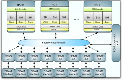
GPU represents a major trend in the recent advance on architecture for high performance computing. GPU processor includes large number of fairly simple cores. We use NVIDIA GT200 architecture (Figure 1) as a candidate for our research.
GT200 is composed of 10 TPCs (Thread ProcessingCluster), each of which includes 3 SMs (Streaming Multiprocessor). Each SM further includes 8 SPs (Streaming Processor) and 2 SFUs (Special Function Unit). If we consider SP as one core, then one GPU processor is comprised of 240 cores.
For Geforce GTX 280 model, with 1296MHz shader clock, the single preci-sion peak performance can reach around 933GFlops. GT280 has 8 64-bit wide GDDR3 memory controllers. With 2214MHz memory clock on GTX 280, the memory bandwidth can reach around 140GB/s. Besides, within each TPC there is a 24KB L1 texture cache and 256KB L2 Texture cache is shared among TPCs.
PC I-Exp re ss 2 .0 x1 6 Interconnect Network DRAM Interface DRAM Interface DRAM Interface DRAM Interface DRAM Interface DRAM Interface DRAM Interface DRAM Interface Texture L2 Texture L2 Texture L2 Texture L2 Texture L2 Texture L2 Texture L2 Texture L2 TPC 0 SM Controller SM Share SM Share SM Share Texture Units Texture L1 TPC 1 SM Controller SM Share SM Share SM Share Texture Units Texture L1 TPC 9 SM Controller SM Share SM Share SM Share Texture Units Texture L1 ... ...
Figure 1: Block Diagram of GT200 GPU
NVIDIA has announced the new generation GPU with code name Fermi. There are a few differences from GT200 generation. First of all, the TPC is removed from the architecture and each SM contains 32 SPs, much more than 8 of GT200. Fermi provides real L1 and L2 cache hierarchy. Double precision computation power increases dramatically for Tesla version Fermi. Since in our present research step, cache effects are ignored, Fermi will be our next research target.
2.2
CUDA Programming Model
The Compute Unified Device Architecture (CUDA) [7] is a C-like abstraction for NVIDIA GPU, and has very good programmability. A CUDA program is composed of host code, which runs on the host CPU, and device code or kernel, which runs on the GPU processor. The device code is first compiled into PTX code, and then into native GPU binary code. In the PTX code, register resource is assumed to be unlimited. The resource allocation and some optimization techniques, such as instruction reordering, are applied when compiling PTX code into binary code.
A typical CUDA program normally creates thousands of threads to hide latency with very light-weight context switch mechanism. These threads are grouped into 1D to 3D blocks, and blocks are grouped into 1D or 2D grids. Threads within one block can share data in shared memory. Programmers need to provide enough number of threads to get good occupancy, so as to hide arithmetic pipeline latency and memory access latency.
Each block is distributed to one SM at execution time. A barrier synchro-nization operation can only be applied to threads in the same block. The basic execution and scheduling units are warps. For GT200 GPU, each warp contains 32 threads. Because processor resources, such as registers and shared memory, are limited, only a limited set of warps can run concurrently on SM, called active warps. We only need to model a few warps running concurrently on each SM to estimate GPU’s performance. Thus, good approximation can be obtained while the problem size is limited.
There are three levels of memory space in CUDA abstraction. Each thread has its own local memory. Each block has a private shared memory partition. All threads can access the global memory , the constant memory space and the texture memory space. Local memory, global memory, constant memory and texture memory are mapped to off-chip DRAM. Both constant memory and texture memory are cached through read-only caches. The per-block shared memory is mapped to on-chip SRAM.
3
Model Setup
In this part, we present an analytical model for GPU GT200 and the key pa-rameters of the model. Then we discuss some performance effects that TEG can demonstrate.
3.1
GPU Analytical Model
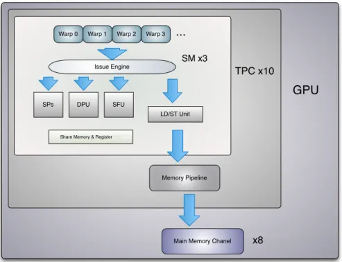
Our model for GT200 GPU is illustrated in Figure 2. In our model, each SM is taken as one processor core. SM is fed with warp instructions. Inside one SM, there are issue engine, shared memory, register file and functional units like SP, DPU, SFU and LD/ST unit. Global memory load/store instructions are issued to LD/ST unit.
Every 2 cycles, the issue engine selects one ready warp instruction from active warps and issues the instruction to the ready functional units according to instruction type. A warp instruction can be be issued when all the source operands are ready. GPU uses a scoreboard mechanism to select the warp with a ready warp instruction. In our model, different scoreboard policies are
6 Lai & Seznec implemented. For each warp, since instructions are issued in program order, if one instruction’s source operands are not ready, all the successive instructions have to wait.
Every three SMs share the same memory pipeline in one TPC, and thus share 1/10 of peak global memory bandwidth. 8 channels connect the device memory chips with the GPU processor and each channel bandwidth cannot exceed 1/8 of peak global memory bandwidth. We do not model the on-die routing of memory requests, since the hardware details have not been disclosed.
TPC x10
Memory Pipeline Issue Engine
Warp 0 Warp 1 Warp 2 Warp 3
Share Memory & Register File
SPs DPU SFU
SM x3
...
LD/ST Unit
GPU
Main Memory Chanel x8
Figure 2: GPU Analytical Model
3.2
Model Parameters
To use the analytical model in TEG, we need to estimate model parameters. In this section, some main parameters are introduced. Much work has been done to understand GPU architecture through benchmarking [11]. Many results and ideas are borrowed from this work.
3.2.1 Instruction Latency
Two types of instruction latency are of interest. One is the execution latency, or cycles that an instruction needs to execute in a functional unit. The other is the issue latency, or cycles that the scheduler has to wait to issue another instruction after issuing one warp instruction. A warp instruction launches 32 operations.
The issue latency is calculated using instruction throughput information. For example, the throughput for integer add is 8 ops/clock. So the issue latency is 32/8 = 4 cycles. When there are enough active warps, the scheduler can issue another warp instruction from another warp in 4 cycles after issuing one integer add instruction. However, when only one single warp is active on SM, the instruction throughput cannot reach the peak performance. According to the instruction throughput of one warp, we can calculate the issue latency of the instruction in one warp. More details are in Section 3.2.2. We illustrate below the methodology that we use to measure instruction execution latency and issue latency.
The typical technique to measure instruction latency is to use the clock() function. The clock() function returns the value of a per-TPC counter. To measure instruction execution latency, we can just put dependent instructions between two clock() function calls. For example, the CUDA code in Listing 1 is translated into PTX code in Listing 2.
t0=c l o c k ( ) ; r1=r1+r3 ; r1=r1+r3 ; . . . r1=r1+r3 ; t1=c l o c k ( ) ;
Listing 1: CUDA Code Example mov . u32 %r6 , %c l o c k ; add . f32 %f4 , %f4 , %f 3 ; add . f32 %f4 , %f4 , %f 3 ; . . . add . f32 %f4 , %f4 , %f 3 ; mov . u32 %r7 , %c l o c k ;
Listing 2: PTX Code Example S2R R3 , SR1 ; SHL R3 , R3 , 0x1 ; FADD32 R4 , R4 , R2 ; FADD32 R4 , R4 , R2 ; . . . FADD32 R4 , R4 , R2 ; S2R R4 , SR1 ; SHL R4 , R4 , 0x1 ;
Listing 3: Disassembly Binary Code Example
The assembly code after compiling PTX code to binary code is in Listing 3. S2R instruction move the clock register to a general purpose register. A depen-dent shift operation after S2R suggests that the clock counter is incremented at half of the shader clock frequency. An extra 28 cycles is introduced because of the dependence between SHL and S2R (24 cycles), and the issue latency of SHL (4 cycles).
8 Lai & Seznec Instruction Type Execution Latency Issue Latency Issue Latency
(multiple warps) (same warp) Integer ADD 24 4 8 Integer MUL (16bit) 24 4 8 Integer MAD (16bit) 24 4 8 Float ADD 24 4 8 Float MUL 24 2 8 Float MAD 24 4 8 Double ADD 48 32 32 Double MUL 48 32 32 Double FMA 48 32 32
Table 1: Arithmetic Instruction Latency
For 21 FADD32 instructions between the two clock measurements, the mea-sured cycles are 514. So the execution latency of FADD32 is
(514 − 28 − 8)/20 ≈ 24.
8 cycles are the issue latency of FADD32 in one warp (Please refer to 3.2.2 for more details).
Some arithmetic instructions’ execution latency and issue latency are listed in Table 1. Since float MUL operation can be issued into both SP and SFU. The instruction has higher throughput and shorter issue latency. In the table we only present the latency for 16 bit integer MUL and MAD, since 32-bit integer MUL and MAD operations are translated into the native 16-bit integer instructions and a few other instructions. In each SM, there is only one SFU which can process double precision arithmetic instructions. Thus, the issue latency is much longer for double precision arithmetic instructions.
3.2.2 Performance Scaling on One SM
In the previous section, the issue latency is calculated assuming several warps are running concurrently. For example, float MAD instruction’s issue latency for multiple warps is 4. But if we run only one warp, then the measured issue latency is 8. And for a global memory load instruction GLD.U32, the issue latency in the same warp is around 60 cycles while the issue latency for multiple warps is a much smaller value and we use 4 cycles in TEG. Similar results are obtained for other arithmetic instructions and memory instructions, which suggests that a warp is occupied to issue one instruction while the scheduler can continue to issue instructions from other warps and the occupied period is normally longer than the waiting time of the scheduler to issue a new instruction from another warp. Thus it is not possible to achieve peak performance with only one active warp on SM even if most nearby instructions in one warp are independent.
After one warp instruction is issued, the scheduler can switch to another warp to execute another instruction without much waiting. However, if the scheduler still issue instructions from the same warp, the longer issue latency is needed. This undocumented behavior may affect performance when there are very few active warps on SM.
3.2.3 Masked instruction
All 32 threads within a warp execute the same warp instruction at a time. When threads of a warp diverge due to a data-dependent branch, they may have different execution path. GPU executes each path in a serial manner. Thus, the warp instruction is masked by a condition dependent on thread index. For masked arithmetic instructions, we find that all behavior remains similar as the un masked behavior. That is to say, all the issue latency and execution latency are the same as those of unmasked arithmetic instructions. For memory operations, since less data needs to be transfered, the latency is shorter and less memory bandwidth is occupied.
3.2.4 Memory Access
We consider the memory access separately from the other instructions because of 3 reasons. First, other functional units belong to one SM only, but each 3 SMs within one TPC share the same memory pipeline and all SMs share the same 8 global memory channels. Second, the scheduler needs to wait around 60 cycles after issuing one global memory instruction to issue another instruction in the same warp, but it can issue another instruction very quickly if it switches to another warp (Refer to Section 3.2.2). Third, memory access has much more complex behavior. For shared memory access, there might be bank conflicts (Section 3.3.3), and then all memory accesses of one half-warp are serialized. For global memory access, there might be coalesced and uncoalesced accesses (Section 3.3.4).
The typical shared memory latency is about 38 cycles and the global memory latency without TLB miss is about 436 to 443 cycles [11].
Let Cmem represent the maximum number of concurrent memory
transac-tions per TPC and it is calculated as follows:
NT P C ∗ NW arp∗ ele_size ∗ Cmem
mem_latency ∗Clk1 = Bpeak Cmem=
Bpeak∗ mem_latency
NT P C∗ NW arp∗ ele_size ∗ Clk
where NT P C, NW arp, ele_size, mem_latency, Clk, and Bpeakdenote the
num-ber of TPCs, the numnum-ber of threads per warp, the accessed data type size, the global memory latency, processor clock frequency, and the peak global memory bandwidth, respectively. For double precision memory transactions, Cmem≈ 18. Thus the number of unfinished double precision memory
transac-tions through the memory pipeline of a TPC cannot exceed 18.
3.3
Performance Effects
3.3.1 Branch Divergence
Masked instructions (Section 3.2.3) are warp instructions with a warp size mask. Each bit of the mask indicates whether the corresponding thread is active to execute the instruction. Threads of the same warp may have different execution path. Since SM has to finish each path in serial and then rejoin, extra execution time is introduced.
10 Lai & Seznec 3.3.2 Instruction Dependence and Memory Access Latency
One of the motivations or advantages of GPU processor is that it can hide latency due to instruction dependence or memory access by forking large number of threads. However, when there are very few active warps, it is possible that at some point, all warps are occupied in issuing instructions. The scheduler is available but none of the active warps can be released. Thus the latency cannot be perfectly hidden and may become an important factor to performance degradation.
3.3.3 Bank Conflicts in Shared Memory
The shared memory is divided in 16 memory modules, or banks, with the bank width of 4 bytes. The bank is interleaved so that successive 4 bytes words in shared memory space are in successive banks. Threads in a half-warp should access different banks to achieve maximum shared memory bandwidth. Other-wise the access is serialized [9], except all threads in a half-warp read the same shared memory address.
For example, the float ADD instruction FADD32 R2, g[A1+0xb], R2;
has a operand g[A1+0xb] located in shared memory. The execution latency is around 74 cycles without bank conflict. If all threads within a half-warp access the same bank, the execution latency becomes about 266 cycles.
3.3.4 Uncoalesced Memory Access in Global Memory
The global memory of GPU has very high access latency comparing to shared memory latency. For global memory accesses of a half-warp, if certain condi-tions are satisfied, the memory transaccondi-tions an be coalesced into one or two transactions. The required conditions depend on GPU hardware and CUDA compute capabilities. The general guideline is that threads of one half-warp should access adjacent memory elements. If the coalesced conditions cannot be met, more memory transactions are needed, introducing much performance loss. For example, if every thread loads 4 bytes from global memory, in the worst case, to serve each thread in the half-warp, 16 separate 32-byte transactions are issued. Thus 87.5% of the global memory bandwidth is wasted.
3.3.5 Chanel Skew in Global Memory
The global memory of GT200 GPU is divided into 8 partitions. The global memory thus can be accessed through 8 channels. The channel width is 256Btyes (32*8B) [9]. Similar as accessing to shared memory, concurrent accesses to global memory should be distributed evenly among all the partitions to achieve high global memory bandwidth. Load imbalance on the memory channels may significantly impair performance. If the application’s memory access pattern has significant imbalance over different channels, much performance degradation will be introduced.
Source Code Binary Code Nvidia CC Functional Simulator Instruction Trace Disassembler Assembly Code Operator Operand Dependence Instruction Analysis Issue Engine Model Functional Units Model Information Collector
Figure 3: Workflow of TEG
4
Workflow of TEG
Based on our timing model of GPU, we have developed the GPU timing esti-mation tool TEG. The workflow of TEG is illustrated in Figure 3. The CUDA source code is first compiled into binary code with NVIDIA compiler collection. The binary code includes the native kernel code that runs on GPU device. Sec-ond, the binary code is disassembled using tool cuobjdump provided by NVIDIA [7]. Third, TEG analyzes the generated assembly code and obtains information such as instruction type, and operands’ type, etc.
We need the actual instruction traces in many cases. The instruction trace can be obtained with detailed GPU simulators, such as Barra[3] or GPGPU-Sim[2]. In our study, the instruction trace is provided by Barra simulator.
So after the third step, the assembly code information and instruction trace are served to issue engine model (see Figure 3). The issue engine model issues all the warp instructions to corresponding functional units model according to the instruction trace and our GPU timing model. At this stage, all runtime timing information can be collected by our information collector.
We can vary the configuration of TEG, such as the active warp number on SM to observe how performance scales from one warp to multiple concurrent warps. We can also compare the performance with or without one bottleneck by choosing whether or not to apply the bottleneck’s effects in TEG. Thus we can quantify how much performance gain we may get by eliminating the bottleneck and programmers can decide whether it is worth the optimization efforts.
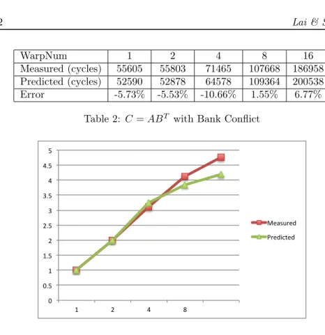
12 Lai & Seznec WarpNum 1 2 4 8 16
Measured (cycles) 55605 55803 71465 107668 186958 Predicted (cycles) 52590 52878 64578 109364 200538 Error -5.73% -5.53% -10.66% 1.55% 6.77%
Table 2: C = ABT with Bank Conflict
0 0.5 1 1.5 2 2.5 3 3.5 4 4.5 5 1 2 4 8 Measured Predicted
Figure 4: C = ABT with Bank Conflict
5
Evaluation
5.1
Dense Matrix Multiplication
We choose one example of dense matrix multiplication in CUDA SDK and to demonstrate the function of TEG, we change C = AB into C = ABT.
C(i, j) =X
k
A(i, k) ∗ B(j, k)
In the implementation, the three matrices A, B and C, are partitioned into 16x16 sub-matrix. The computation for a C sub-matrix is assigned to a CUDA block. A block is composed of 256 (16x16) threads and each thread computes one element in the C sub-matrix. In the CUDA kernel, at each step, a block of threads load the A and B sub-matrices first into shared memory. After a barrier synchronization of the block, each thread loads A(i, k) and B(j, k) from shared memory, and accumulates the multiplication result to C(i, j).
However, since a half-warp of threads, load B(j, k), B(j + 1, k), . . . , B(j + 15, k), for a shared memory allocation like B[16][16], all the 16 elements will reside in the same bank and there would be bank conflicts in the shared memory. In the following experiment, we assign each warp with the same amount of workload and run 1 to 16 warps concurrently on one SM. We use clock() function to measure the execution time on device of one block, since the barrier synchronization is only applicable within one block. And for multiple blocks’ total execution time, we use the measured host time to calculate the device
WarpNum 1 2 4 8 16 Measured (cycles) 17511 17291 18330 23228 33227 Predicted (cycles) 16746 17528 19510 23630 34896 Error -4.57% 1.35% 6.05% 1.70% 4.78%
Table 3: C = ABT Modified
execution time. For example, when there are 30 blocks, each SM can be assigned one block and when there are 60 blocks, each SM has two blocks to execute. Then we compare the host time for the two configurations and calculate the cycles for 2 blocks (16 warps) to finish on the SM.
The measured and predicted execution time of 1 to 16 concurrent warps on one SM is illustrated in Table 2. Then we normalize the execution time with the workload and show the speed up from 1 to 16 active warps on each SM in Figure 4. 0 1 2 3 4 5 6 7 8 9 1 2 4 8 16 Measured Predicted Figure 5: C = ABT Modified
For GPU performance optimization, programmers often come to the question that how much performance loss due to one performance degradation factor. With TEG, it is fairly easy to answer the question. We just need to change the configuration. In this case, in the tool, we just assume all shared memory accesses are conflict-free. Thus we can estimate the performance without shared memory bank conflict, which is illustrated in Figure 5 and Table 3.
We then modified the CUDA code to eliminate bank conflicts and compare the result with TEG’s output. The comparison shows very good approximation.
5.2
Lattice QCD
Quantum chromodynamics (QCD) is the physical theory for strong interac-tions and lattice QCD is a numerical approach to QCD theory. Lattice QCD simulation is one of the challenging problems for high performance computing community.
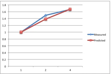
14 Lai & Seznec WarpNum 1 2 4
Measured (cycles) 51053 68383 122430 Predicted (cycles) 46034 66674 110162 Error -10.90% -2.56% -11.14% Table 4: Hopping_Matrix kernel with Uncoalesced Accesses
We select one kernel in Hopping_Matrix routine [5] as our example. The input of the Hopping_Matrix kernel include the spinor field, the gauge field, the output is the result spinor field. The spinor field resides on the 4D space-time site and is represented by a 3x4 complex matrix data structure. The gauge field on the link connecting neighbor sites is implemented as a 3x3 complex matrix. The half spinor filed is represented by a 3x2 complex matrix, which is the temporary data generated on each of 8 space-time directions for one full spinor.
The functionality of the kernel is not important to our discussion. Instead, the memory layout is of interest. In the first version of our implementation, all the data is organized in array of structures. This is typical data layout for conventional processors to obtain good cache hit rate. However, GPU has much more concurrent threads. Normally different threads are assigned with different data structures. So the accesses of the threads in a warp have a long stride of the size of the data structure. Thus, accesses to global memory cannot be coalesced. The predicted and measured execution results are illustrated in Table 4 and Figure 6. Since each thread occupies much register resource, the active warp number is limited.
0 0.2 0.4 0.6 0.8 1 1.2 1.4 1.6 1.8 1 2 4 Measured Predicted
Figure 6: Hopping_Matrix kernel with Uncoalesced Accesses
If we reorganize the data layout into structure of arrays, the memory accesses of threads in a warp would be adjacent. Thus they can be coalesced. The result is shown in Table 5 and Figure 7. This case also shows that TEG can easily demonstrate the performance loss due to performance bottlenecks, such as uncoalesced memory accesses.
WarpNum 1 2 4 Measured (cycles) 37926 47038 73100 Predicted (cycles) 36202 45204 68104 Error -4.76% -4.06% -7.34% Table 5: Hopping_Matrix kernel with Coalesced Accesses
0 0.5 1 1.5 2 2.5 1 2 4 Measured Predicted
Figure 7: Hopping_Matrix kernel with Coalesced Accesses
6
Conclusion
In our paper, we present our timing model for GT200 GPU and a timing esti-mation tool TEG. With the timing model and the assembly code as input, TEG can estimate GPU cycle-approximate performance. Evaluation cases show that TEG can get very close performance approximation. Especially, TEG has good approximation for applications with very few active warps on SM. Thus we could better understand GPU’s performance result and quantify bottlenecks’ performance effects. Present profiling tools can only provide programmers with bottleneck statistics, like number of shared memory bank conflict, etc. TEG allows programmers to understand how much performance one bottleneck can impair and forsee the benefit of eliminating the bottleneck.
The main limitation is that TEG cannot handle the situation when there is much memory traffic and a lot of memory contention occurs because we lack the knowledge of detailed on-die memory controller organization and the analysis is far too complicated for our analysis method. Our future plan includes studying the new Fermi architecture and introducing cache effects into our model.
References
[1] S. S. Baghsorkhi, M. Delahaye, S. J. Patel, W. D. Gropp, and W.-m. W. Hwu. An adaptive performance modeling tool for gpu architectures. SIG-PLAN Not., 45:105–114, January 2010.
16 Lai & Seznec [2] A. Bakhoda, G. L. Yuan, W. W. L. Fung, H. Wong, and T. M. Aamodt. Analyzing cuda workloads using a detailed gpu simulator. In ISPASS, pages 163–174. IEEE, 2009.
[3] S. Collange, M. Daumas, D. Defour, and D. Parello. Barra: A parallel functional simulator for gpgpu. In 2010 18th Annual IEEE/ACM Interna-tional Symposium on Modeling, Analysis and Simulation of Computer and Telecommunication Systems, page 351Ð360. IEEE, 2010.
[4] S. Hong and H. Kim. An analytical model for a gpu architecture with memory-level and thread-level parallelism awareness. SIGARCH Comput. Archit. News, 37(3):152–163, 2009.
[5] K. Z. Ibrahim and F. Bodin. Efficient simdization and data management of the lattice qcd computation on the cell broadband engine. Sci. Program., 17(1-2):153–172, 2009.
[6] Y. Kim and A. Shrivastava. Cumapz: a tool to analyze memory access patterns in cuda. In Design Automation Conference (DAC), 2011 48th ACM/EDAC/IEEE, page 128Ð133. IEEE, 2011.
[7] NVIDIA. NVIDIA CUDA C Programming Guide 4.0. [8] Opencl. http://www.khronos.org/opencl/.
[9] G. Ruetsch and P. Micikevicius. Optimizing matrix transpose in cuda. 2009.
[10] S. Ryoo, C. I. Rodrigues, S. S. Stone, S. S. Baghsorkhi, S.-Z. Ueng, J. A. Stratton, and W. mei W. Hwu. Program optimization space pruning for a multithreaded gpu. In CGO ’08: Proceedings of the sixth annual IEEE/ACM international symposium on Code generation and optimiza-tion, pages 195–204, New York, NY, USA, 2008. ACM.
[11] H. Wong, M.-M. Papadopoulou, M. Sadooghi-Alvandi, and A. Moshovos. Demystifying gpu microarchitecture through microbenchmarking. In IS-PASS’10, pages 235–246, 2010.
[12] Y. Zhang and J. D. Owens. A quantitative performance analysis model for gpu architectures. In Proceedings of the 17th IEEE International Sympo-sium on High-Performance Computer Architecture (HPCA 17), Feb. 2011.