HAL Id: hal-01238445
https://hal.archives-ouvertes.fr/hal-01238445
Submitted on 9 Dec 2015
HAL is a multi-disciplinary open access
archive for the deposit and dissemination of
sci-entific research documents, whether they are
pub-lished or not. The documents may come from
teaching and research institutions in France or
abroad, or from public or private research centers.
L’archive ouverte pluridisciplinaire HAL, est
destinée au dépôt et à la diffusion de documents
scientifiques de niveau recherche, publiés ou non,
émanant des établissements d’enseignement et de
recherche français ou étrangers, des laboratoires
publics ou privés.
Copyright
Three generalizations of the FOCUS constraint
Nina Narodytska, Thierry Petit, Mohamed Siala, Toby Walsh
To cite this version:
Nina Narodytska, Thierry Petit, Mohamed Siala, Toby Walsh. Three generalizations of the FOCUS
constraint. Constraints, Springer Verlag, 2016, 21 (4), pp.459-532. �10.1007/s10601-015-9233-7�.
�hal-01238445�
(will be inserted by the editor)
Three Generalizations of the FOCUS Constraint
Nina Narodytska · Thierry Petit · MohamedSiala · Toby Walsh
Received: date / Accepted: date
Abstract The FOCUSconstraint expresses the notion that solutions are concentrated. In practice, this constraint suffers from the rigidity of its semantics. To tackle this is-sue, we propose three generalizations of the FOCUSconstraint. We provide for each one a complete filtering algorithm. Moreover, we propose ILP and CSP decomposi-tions.
1 Introduction
Many discrete optimization problems have constraints on the objective function. Be-ing able to represent such constraints is fundamental to deal with many real world industrial problems. Constraint programming is a rich paradigm to express and filter such constraints. In particular, several constraints have been proposed for obtaining well-balanced solutions [9, 17, 11]. Recently, the FOCUS constraint [12] was intro-duced to express the opposite notion. It captures the concept of concentrating the high values in a sequence of variables to a small number of intervals. We recall its definition. Throughout this paper, X = [x0, x1, . . . , xn−1] is a sequence of integer
variables and si,j is a sequence of indices of consecutive variables in X, such that
Nina Narodytska
Samsung Research America, Mountain View, USA E-mail: [email protected]
Thierry Petit
School of Business, Worcester Polytechnic Institute, Worcester, USA LINA-CNRS, Mines-Nantes, INRIA, Nantes, France
E-mail: [email protected], [email protected] Mohamed Siala
Insight Centre for Data Analytics, University College Cork, Ireland E-mail: [email protected]
Toby Walsh
NICTA and UNSW, Sydney, Australia E-mail: [email protected]
si,j = [i, i + 1, . . . , j], 0 ≤ i ≤ j < n. For each variable x, we denote by D(x) the
domain of x and finally, we let |E| be the size of a collection E.
Definition 1 ([12]) Let ycbe a variable. Let k and len be two integers, 1 ≤ len ≤
|X|. An instantiation of X ∪ {yc} satisfies FOCUS(X, yc, len, k ) iff there exists a set
SXof disjoint sequences of indices si,jsuch that three conditions are all satisfied:
1. |SX| ≤ yc
2. ∀xl∈ X, xl> k ⇔ ∃si,j∈ SXsuch that l ∈ si,j
3. ∀si,j∈ SX, j − i + 1 ≤ len
Example 1 Let k = 0, D(yc) = {2}, X = [x0, .., x5], D(x0) = {1}, D(x1) = {3},
D(x2) = {1}, D(x3) = {0}, D(x4) = {1}, D(x5) = {0}. If len = 6, then
FOCUS(X, yc, len, k ) is satisfied since we can have 2 disjoint sequences of length
≤ 6 of consecutive variables with a value strictly positive, i.e., hx0, x1, x2i, and hx4i.
If len = 2, FOCUS(X, yc, len, k ) becomes violated since it is impossible to include
all the strictly positive variables in X with only 2 sequences of length ≤ 2.
FOCUScan be used in various contexts including cumulative scheduling problems where some excesses of capacity can be tolerated to obtain a solution [12]. In a cumu-lative scheduling problem, we are scheduling activities, and each activity consumes a certain amount of some resource. The total quantity of the resource available is lim-ited by a capacity. Excesses can be represented by variables [4]. In practice, excesses might be tolerated by, for example, renting a new machine to produce more resource. Suppose the rental price decreases proportionally to its duration: it is cheaper to rent a machine during a single interval than to make several rentals. On the other hand, rental intervals have generally a maximum possible duration. FOCUScan be set to concentrate (non null) excesses in a small number of intervals, each of length at most len.
Unfortunately, the usefulness of FOCUSis hindered by the rigidity of its seman-tics. For example, we might be able to rent a machine from Monday to Sunday but not use it on Friday. It is a pity to miss such a solution with a smaller number of rental intervals because FOCUSimposes that all the variables within each rental in-terval take a high value. Moreover, a solution with one rental inin-terval of two days is better than a solution with a rental interval of four days. Unfortunately, FOCUSonly considers the number of disjoint sequences, and does not consider their length.
Consider a simple example of a resource R with a capacity equal to 3. We use a sequence of variables [x0, .., x9] to model the amount of consumed capacity at time
unit i (e.g., one day). Suppose that some activities are already scheduled on R such that the current assignment of [x0, .., x9] is:
[x0, .., x9]: 4 2 4 2 2 0 0 0 0 0
In this example, the first day requires a capacity equal to 4, the second requires 2, etc. The standard capacity constraints are exceeded in x0and x2.
Suppose that an additional activity has to be scheduled on this resource. The new activity has a duration of 5 days, each of which consumes 2 units of capacity. The followings sequence (denoted S1) shows the new resource consumption if we start
the new activity at x1.The red values show the new capacity requirement after adding
[x0, .., x9] 4 4 6 4 4 2 0 0 0 0
The new sequence S1 satisfies FOCUS(X, [1, 1], 5, 3) since we have only one
sub-sequence where the capacity constraints are all exceeded (i.e. hx0, x1, x2, x3, x4i).
However, there is no possible way to satisfy the constraint if the length is equal to 3. FOCUS(X, [1, 1], 3, 3) is violated.
Consider now a form of relaxation by allowing some variables in the sub-sequences to have values that do not exceed capacity. In this case, a solution is possible if we start the additional activity at x5(denoted S2). That is:
[x0, .., x9]: 4 2 4 2 2 2 2 2 2 2
The unique subsequence in S2 where some capacity constraints are exceeded is
hx0, x1, x2i. Relaxing FOCUSin this sense might be very useful in practice.
Consider now again FOCUS(X, [2, 2], 5, 3). The two solutions S1and S2satisfy the
constraint. Notice that there is 6 capacity excesses in S1(i.e., in x0, x1, x2, x3, x4)
and only 2 in S2(i.e., in x0and x2). Therefore, one might prefer S2since we have less
capacity excesses although the project ends later. Restricting the length subsequences to be at most 2 in this example will prune the first solution.
We tackle those issues in this paper by means of three generalizations of FOCUS.
SPRINGYFOCUStolerates within each sequence si,j ∈ SXsome values v ≤ k . To
keep the semantics of grouping high values, their number is limited in each si,j by
an integer argument. WEIGHTEDFOCUS adds a variable to count the length of se-quences, equal to the number of variables taking a value v > k . The most generic one, WEIGHTEDSPRINGYFOCUS, combines the semantics of SPRINGYFOCUS and WEIGHTEDFOCUS. Propagating such constraints, i.e. complementary to an objective function, is well-known to be important [10, 18]. We present and experiment with filtering algorithms and decompositions therefore for each constraint. One of the de-compositions highlights a relation between SPRINGYFOCUS and a tractable Integer Linear Programming (ILP) problem.
The rest of this paper is organized as follows : We give in Section 2 a short back-ground on Constraint Programming and Network Flows. Next, in Sections 3, 4 and 5, we present three generations of the FOCUSconstraint (denoted by SPRINGYFOCUS, WEIGHTEDFOCUS, and WEIGHTEDSPRINGYFOCUSrespectively). In particular, we provide complete filtering algorithms as well as ILP formulations and CSP decom-positions. Finally, we evaluate, in Section 6, the impact of the new filtering compared to decompositions.
2 Background
A constraint satisfaction problem (CSP) is defined by a set of variables, each with a finite domain of values, and a set of constraints specifying allowed combinations of values for subsets of variables. For each variable x, we denote by min(x) (respec-tively max(x)) the minimum (respec(respec-tively maximum) value in D(x). Given a con-straint C, we denote by Scope(C) the set of variables constrained by C. A solution is an assignment of values to the variables satisfying the constraints.
Constraint solvers typically explore partial assignments enforcing a local consis-tency property using either specialized or general purpose filtering algorithms [16]. A filtering algorithm (called also a propagator) is usually associated with one constraint, to remove values that cannot belong to an assignment satisfying this constraint. A lo-cal consistency formally characterizes the impact of filtering algorithms. The two most used local consistencies are domain consistency (DC) and bound consistency (BC). A support for a constraint C is a tuple that assigns a value to each variable in Scope(C) from its domain which satisfies C. A bounds support for a constraint C is a tuple that assigns a value to each variable in Scope(C) which is between the maximum and minimum in its domain which satisfies C. A constraint C is domain consistent(DC) if and only if for each variable xi ∈Scope(C), every value in the
cur-rent domain of xi belongs to a support. A constraint C is bounds consistent (BC) if
and only if for each variable xi ∈Scope(C), there is a bounds support for the
maxi-mum and minimaxi-mum value in its current domain. A CSP isDC/BCif and only if each constraint isDC/BC. Regarding FOCUS, a complete filtering algorithm (i.e. achieving domain consistency) is proposed in [12] running in O(n) time complexity.
A flow network is a weighted directed graph G = (V, E) where each edge e has a capacity between non-negative integers l(e) and u(e), and an integer cost w(e). A feasible flowin a flow network between a source (s) and a sink (t), (s, t)-flow, is a function f : E → Z+ satisfying two conditions: f (e) ∈ [l(e), u(e)], ∀e ∈ E and
the flow conservation law that ensures that the amount of incoming flow should be equal to the amount of outgoing flow for all nodes except the source and the sink. The valueof a (s, t)-flow is the amount of flow leaving the sink s. The cost of a flow f is
w(f ) =P
e∈Ew(e)f (e). A minimum cost flow is a feasible flow with the minimum
cost [1].
3 Springy FOCUS 3.1 Definition
In Definition 1, each sequence in SX contains exclusively values v > k. In many
practical cases, this property is too strong.
Consider one simple instance of the problem in the introduction (depicted in Fig-ure 1) for a given resource of capacity 3. Each variable xi∈ X represents the resource
consumption and is defined per unit of time (e.g., one day). Initially, 4 activities are fixed (drawing A) as follows:
1. Activity 1 starts at day 0 and requires 4 units of capacity during one day 2. Activity 2 starts at day 1 and requires 2 units of capacity during one day 3. Activity 3 starts at day 2 and requires 4 units of capacity during one day 4. Activity 4 starts at day 3 and requires 2 units of capacity during two days
Suppose now that an additional activity with 2 units of capacity and a duration of 5 days remains to be scheduled. Suppose also that the domain of the starting time of the new activity is D(st) = [1, 5]. If FOCUS(X, yc = 1, 5, 3) is imposed then this
Fig. 1 Introducing SPRINGYFOCUS
Example of a resource with capacity equal to 3. Each day is represented by one unit in the horizontal axis. The capacity usage is represented by the vertical axis. (A) Problem with 4 fixed activities: activity 1 scheduled on day 0 with 4 units of capacity; activity 2 scheduled on day 1 with 2 units of capacity; activity 3 scheduled on day 2 with 4 units of capacity; and activity 4 scheduled on days 3 and 4 with 2 units of capacity each. An additional activity of length 5 should start from time 1 to 5 (i.e. the domain of the starting time of the new activity is D(st)=[1,5]). (B) Solution satisfying FOCUS(X, [1, 1], 5, 3), with a new machine rented for 5 days. (C) Practical solution violating FOCUS(X, [1, 1], 5, 3), with a new machine rented for 3 days but not used on the second day.
Assume now that the new machine may not be used every day. Solution (C) gives one rental of 3 days instead of 5. Furthermore, if len = 4 the problem will have no solution using FOCUS, while this latter solution still exists in practice. This is paradoxical, as relaxing the condition that sequences in the set SX of Definition 1
take only values v > k deteriorates the concentration power of the constraint. There-fore, we propose a soft relaxation of FOCUS, where at most h values less than k are tolerated within each sequence in SX.
Definition 2 Let ycbe a variable and k , len, h be three integers, 1 ≤ len ≤ |X|, 0 ≤
h < len − 1. An instantiation of X ∪ {yc} satisfies SPRINGYFOCUS(X, yc, len, h, k )
iff there exists a set SXof disjoint sequences of indices si,jsuch that four conditions
are all satisfied: 1. |SX| ≤ yc
2. ∀xl∈ X, xl> k ⇒ ∃si,j∈ SXsuch that l ∈ si,j
3. ∀si,j∈ SX, j − i + 1 ≤ len, xi > k and xj > k.
4. ∀si,j∈ SX, |{l ∈ si,j, xl≤ k }| ≤ h
3.2 Filtering Algorithm
Bounds consistency(BC) on SPRINGYFOCUS is equivalent to domain consistency: any solution can be turned into a solution that only uses the lower bound min(xl) or
the upper bound max(xl) of the domain D(xl) of each xl∈ X (this observation was
made for FOCUS[12]). Thus, we propose aBCalgorithm. The first step is to traverse X from x0to xn−1, to compute the minimum possible number of disjoint sequences
in SX(a lower bound for yc), the focus cardinality, denoted fc(X). We give a formal
definition.
Definition 3 Focus cardinality
focus cardinality of any subsequence s ⊂ X, denoted fc(s), is defined as follows:
fc(s) = min
ω∈D(yc)
{SPRINGYFOCUS(s, ycω, len, h, k ) is satisfiable | D(ycω) = {ω}}
Definition 4 Given xl∈ X, we consider three quantities.
1. p(xl, v≤) is the focus cardinality of [x0, x1, . . . , xl], assuming xl ≤ k , and
∀si,j∈ S[x0,x1,...,xl], j 6= l.
2. pS(xl, v≤), 0 < l < n − 1, is the focus cardinality of [x0, x1, . . . , xj], where l <
j < n, assuming xl ≤ k and ∃i, 0 ≤ i < l, si,j ∈ S[x0,x1,...,xj]. pS(x0, v≤) =
pS(xn−1, v≤) = n + 1.
3. p(xl, v>) is the focus cardinality of [x0, x1, . . . , xl] assuming xl> k .
Any quantity is equal to n + 1 if the domain D(xl) of xlmakes impossible the
considered assumption.
We shall use the above notations throughout the paper. Property 1 fc(X) = min(p(xn−1, v≤), p(xn−1, v>)).
Proof By construction from Definitions 2 and 4. ut
To compute the quantities of Definition 4 for xl ∈ X we use two additional
measures.
Definition 5 plen(xl) is the minimum length of a sequence in S[x0,x1,...,xl]
contain-ing xl among instantiations of [x0, x1, . . . , xl] where the number of sequences is
fc([x0, x1, . . . , xl]). plen(xl)=0 if ∀si,j∈ S[x0,x1,...,xl], j 6= l.
Definition 6 card (xl) is the minimum number of values v ≤ k in the current
se-quence in S[x0,x1,...,xl], equal to 0 if ∀si,j ∈ S[x0,x1,...,xl], j 6= l. card (xl) assumes
that xl> k. It has to be decreased it by one if xl≤ k.
Proofs of following recursive Lemmas 1 to 4 omit the obvious cases where quan-tities take the default value n + 1.
Lemma 1 (initialization) p(x0, v≤) = 0 if min(x0) ≤ k, and n + 1 otherwise;
pS(x0, v≤) = n + 1; p(x0, v>) = 1 if max(x0) > k and n + 1 otherwise; plen(x0)
= 1 if max(x0) > k and 0 otherwise; card (x0) = 0.
Proof From item 4 of Definition 2, a sequence in SXcannot start with a value v ≤ k.
Thus, pS(x0, v≤) = n + 1 and card (x0) = 0. If x0can take a value v > k then by
Definition 4, p(x0, v>) = 1 and plen(x0) = 1. ut
We now consider a variable xl∈ X, 0 < l < n.
Lemma 2 (p(xl, v≤)) If min(xl) ≤ k then p(xl, v≤) =
Proof If min(xl) ≤ k then pS(xl−1, v≤) must not be considered: it would imply
that a sequence in SX ends by a value v ≤ k for xl−1. From Property 1, the focus
cardinality of the previous sequence is min(p(xl−1, v≤), p(xl−1, v>)). ut
Lemma 3 (pS(xl, v≤)) If min(xi) > k, pS(xi, v≤) = n + 1.
Otherwise, ifplen(xi−1) ∈ {0, len − 1, len} ∨ card (xi−1) = h then pS(xi, v≤) =
n + 1, else pS(xi, v≤) = min(pS(xi−1, v≤), p(xi−1, v>)).
Proof If min(xi) ≤ k we have three cases to consider. (1) If either plen(xi−1) = 0
or plen(xi−1) = len then from item 3 of Definition 2 a sequence in SX cannot start
with a value vi ≤ k: pS(xi, v≤) = n + 1. (2) If plen(xi−1) = len − 1 then from
Definition 2 the current variable xicannot end the sequence with a value vi≤ k. (3)
Otherwise, from item 3 of Definition 2, p(xi−1, v≤) is not considered. Thus, from
Property 1, pS(xi, v≤) = min(pS(xi−1, v≤), p(xi−1, v>)). ut
Lemma 4 (p(xl, v>)) If max(xl) ≤ k then p(xl, v>)=n + 1.
Otherwise, Ifplen(xl−1) ∈ {0, len}, p(xl, v>) = min(p(xl−1, v>)+1, p(xl−1, v≤)+
1), else p(xl, v>) = min(p(xl−1, v>), pS(xl−1, v≤), p(xl−1, v≤) + 1).
Proof If plen(xl−1) ∈ {0, len} a new sequence has to be considered: pS(xl−1, v≤)
must not be considered, from item 3 of Definition 2. Thus, p(xl, v>) =
min(p(xl−1, v>) + 1, p(xl−1, v≤) + 1). Otherwise, either a new sequence has to
be considered (p(xl−1, v≤) + 1) or the value is equal to the focus cardinality of the
previous sequence ending in xl−1. ut
Proposition 1 (plen(xl)) If min (pS(xl−1, v≤), p(xl−1, v>)) < p(xl−1, v≤) + 1 ∧
plen (xl−1) < len then plen(xl) = plen(xl−1) + 1. Otherwise, if p(xl, v>)) < n + 1
thenplen(xl) = 1, else plen(xl) = 0.
Proof By construction from Definition 5 and Lemmas 1, 2, 3 and 4. ut
Proposition 2 (card (xl)) If plen(xl) = 1 then card (xl) = 0. Otherwise, if
p(xl, v>) = n + 1 then card (xl) = card (xl−1) + 1, else card (xl) = card (xl−1).
Proof By construction from Definition 5, 6 and Lemmas 1 and 4. ut
Algorithm 1 implements the lemmas with pre[l][0][0] = p(xl, v≤), pre[l][0][1] =
pS(xl, v≤), pre[l][1] = p(xl, v>), pre[l][2] = plen(xl), pre[l][3] = card (xl).
The principle of Algorithm 2 is the following. First, lb = f c(X) is computed with xn−1. We execute Algorithm 1 from x0to xn−1and conversely (arrays pre and suf ).
We thus have for each quantity two values for each variable xl. To aggregate them, we
implement regret mechanisms directly derived from Propositions 1 and 2, according to the parameters len and h. Line 4 is optional but it avoids some work when the variable ycis fixed, thanks to the same property as FOCUS (see [12]). Algorithm 2
performs a constant number of traversals of the set X. Its time complexity is O(n), which is optimal.
Algorithm 1: MINCARDS(X, len, k , h): Integer matrix
1 pre := new Integer[|X|][4][] ; 2 for l ∈ 0..n − 1 do
3 pre[l][0] := new Integer[2];
/* Initialization from Lemma 1 */
4 if min(x0) ≤ k then 5 pre[0][0][0] := 0 ; 6 else 7 pre[0][0][0] := n + 1 ; 8 pre[0][0][1] := n + 1 ; 9 if max(x0) > k then 10 pre[0][1] := 1 ; 11 else 12 pre[0][1] := n + 1 ; 13 if max(x0) > k then 14 pre[0][2] := 1 ; 15 else 16 pre[0][2] := 0 ; 17 pre[0][3] := 0 ; 18 for l ∈ 1..n − 1 do /* Lemma 2 */ 19 if min(xl) ≤ k then
20 pre[l][0][0] := min(pre[l − 1][0][0], pre[l − 1][1]) ; 21 else 22 pre[l][0][0] := n + 1 ; /* Lemma 3 */ 23 if min(xl) > k then 24 pre[l][0][1] := n + 1 ; 25 else
26 if pre[l − 1][2] ∈ {0, len − 1, len} ∨ pre[l − 1][3] = h then
27 pre[l][0][1] := n + 1 ;
28 else
29 pre[l][0][1] := min(pre[l − 1][0][1], pre[i − 1][0][0]) ;
/* Lemma 4 */
30 if max(xl) ≤ k then 31 pre[l][1] := n + 1 ; 32 else
33 if pre[l − 1][2] ∈ {0, len} then
34 pre[l][1] = min(pre[l − 1][1] + 1, pre[l − 1][0][0] + 1) ;
35 else
36 pre[l][1] = min(pre[l − 1][1], pre[l − 1][0][1], pre[l − 1][0][0] + 1)
/* Proposition 1 */
37 if min (pre[l − 1][0][1], pre[l − 1][1]) < pre[l − 1][0][0] + 1 ∧ pre[l − 1][2] < len then 38 pre[l][2] = pre[l − 1][2] + 1 ; 39 else 40 if pre[l][1] < n + 1 then 41 pre[l][2] := 1 ; 42 else 43 pre[l][2] := 0 ; /* Proposition 2 */ 44 if pre[l][2] = 1 then 45 pre[l][3] := 0 ; 46 else 47 if pre[l][1] = n + 1 then 48 pre[l][3]) := pre[l − 1] + 1; 49 else 50 pre[l][3]) := pre[l − 1] ; 51 return pre;
Algorithm 2: FILTERING(X, yc, len, k , h): Set of variables
1 pre := MINCARDS(X, len, k, h) ;
2 Integer lb := min(pre[n − 1][0][0], pre[n − 1][1]); 3 if min(yc) < lb then D(yc) := D(yc) \ [min(yc), lb[ ; 4 if min(yc) = max(yc) then
5 suf := MINCARDS([xn−1, xn−2, . . . , x0], len, k, h) ; 6 for l ∈ 0..n − 1 do
7 if pre[l][0][0] + suf [n − 1 − l][0][0] > max(yc) then 8 Integer regret := 0; Integer add := 0;
9 if pre[l][1] ≤ pre[l][0][1] then add := add + 1 ;
10 if suf [n − 1 − l][1] ≤ suf [n − 1 − l][0][1] then add:=add+1 ;
11 if pre[l][2] + suf [n − 1 − l][2] − 1 ≤ len ∧
pre[l][3] + suf [n − 1 − l][3] + add − 1 ≤ h then regret := 1 ;
12 if pre[l][0][1] + suf [n − 1 − l][0][1] − regret > max(yc) then D(xi) :=
D(xi)\ [min(xi), k] ; 13 Integer regret := 0;
14 if pre[l][2] + suf [n − 1 − l][2] − 1 ≤ len ∧ pre[l][3] + suf [n − 1 − l][3] − 1 ≤ h then regret := 1 ;
15 if pre[l][1] + suf [n − 1 − l][1] − regret > max(yc) then 16 D(xi) := D(xi)\ ]k, max(xi)];
17 return X ∪ {yc};
3.3 Integer Linear Programming formulation
In this section we present a new Integer Linear Programming (ILP) formulation of SPRINGYFOCUS. This connection highlights a relation between SPRINGYFOCUS
and a tractable ILP problem. It adds one more constraint to a bag of constraints that can be propagated using shortest path or network flow reformulations [13, 14, 6].
We first present a bounds disentailment technique. We use the following notations from [12].
Definition 7 ([12]) Given an integer k , a variable xl∈ X is:
– Penalizing, (Pk), iff min(xl) > k.
– Neutral, (Nk), iff max(xl) ≤ k.
– Undetermined, (Uk), otherwise.
We say xl∈ Pkiff xlis labelled Pk, and similarly for Ukand Nk.
The main observation behind the reformulation is that we can relax the require-ment of disjointness of sequences in SX (Definition 2) and find a solution of the
SPRINGYFOCUSconstraint. This solution can be transformed into a solution where sequences in SXare disjoint as we can truncate the overlaps. If we drop the
require-ment of disjointness of sequences in SXthen we only need to consider at most n
pos-sible sequences si,i+leni−1, i ∈ {0, 1, . . . , n − 1}, xiand xi+leni−1are not neutral,
and leni is the maximal possible length of a sequence that starts at the ith position.
Note that leni does not have to be equal to len as si,i+leni−1 can cover at most h
variables that take values less than or equal to k. We call the set of these sequences So
Fig. 2 The set of possible sequences in SXfrom Example 2.
Example 2 Consider X = [x0, x1. . . , x8] and SPRINGYFOCUS(X, [3, 3], 3, 1, 0)
with D(x0) = D(x2) = D(x5) = D(x7) = D(x8) = {1}, D(x1) = D(x3) =
D(x4) = 0 and D(x6) = {0, 1}. There are 9 sequences to consider as there are
9 variables. We have 5 valid sequences that are schematically shown in black in Figure 2(a). Hence, SXo = {s0,2, s5,7, s6,8, s7,8, s8,8}. The remaining 4 sequences,
s1,2, s2,3, s3,3and s4,6, are discarded, as a sequence should not start(finish) at a
neu-tral variable. We highlighted invalid sequences in grey.
We denote the SPRINGYFOCUSconstraint without the disjointness requirement SPRINGYFOCUSOVERLAP. More formally we define SPRINGYFOCUSOVERLAPas follows.
Definition 8 Let yc be a variable and k , len, h be three integers, 1 ≤
len ≤ |X|, 0 ≤ h < len − 1. An instantiation of X ∪ {yc} satisfies
SPRINGYFOCUSOVERLAP(X, yc, len, h, k ) iff there exists a set SX ⊆ SXo of
se-quences (not necessary disjoint) of indices si,jsuch that four conditions are all
satis-fied:
1. |SX| ≤ yc
3. ∀si,j∈ SX, j − i + 1 ≤ len, xi > k and xj > k
4. ∀si,j∈ SX, |{l ∈ si,j, xl≤ k }| ≤ h
Lemma 5 SPRINGYFOCUS(X, yc, len, h, k ) has a solution iff
SPRINGYFOCUSOVERLAP(X, yc, len, h, k ) has a solution.
Proof ⇐ Let I[X ∪ {yc}] be a solution of SPRINGYFOCUSOVERLAP. We order
se-quences in SXby their starting points and process them in this order. Let si,i+leni−1
and sj,j+lenj−1 be the first two consecutive sequences in SX that overlap. We
up-date SX. First, we remove sj,j+lenj−1: SX = SX\ {sj,j+lenj−1}. Consider a
se-quence si+leni,j+lenj−1. By definition, xj+lenj−1 > k . If si+leni,j+lenj−1 has a
prefix that contains only neutral variables then we cut it from the sequence and ob-tain si0,j+len
j−1. We add this sequence to our set: SX = SX∪ {si0,j+lenj−1}. So, we
cut the prefix of sj,j+lenj−1to avoid the overlap and made sure that the new sequence
does not start or end at a neutral variable. This does not change the cardinality |SX|.
We continue this procedure for the rest of the sequences. The updated set SX covers
the same set of penalizing variables as the original set and all sequences are disjoint. ⇒ Let I[X ∪{yc}] be a solution of SPRINGYFOCUS. We extend each sequence to
its maximal length to the right. This gives a solution of SPRINGYFOCUSOVERLAP. u
t
Example 3 Consider SPRINGYFOCUSOVERLAP from Example 2. SX =
{s0,2, s5,7, s7,8} is a possible solution (dashed lines in Figure 2(a)). We
can cut the prefix of s7,8 to avoid an overlap between s5,7 and s7,8. We
obtain s8,8 which does not start or finish at a neutral variable. Hence,
SX = (SX∪ {s8,8}) \ {s7,8} = {s0,2, s5,7, s8,8}.
Thanks to Lemma 5 we build an ILP reformulation for
SPRINGYFOCUSOVERLAP, solve this ILP and transform to a solution of the SPRINGYFOCUS constraint. We introduce one Boolean variable svi for each
sequence in SXo. We can write an integer linear program:
Minimize X i:si,i+leni∈So X svi (1) X {svi:xj∈si,i+leni−1} svi ≥ 1 ∀xj ∈ Pk (2) svi∈ {0, 1} ∀svi. (3)
Lemma 6 SPRINGYFOCUSOVERLAP(X, yc, len, h, k ) is satisfiable iff the ILP
sys-tem 1–3 has a solution of cost less than or equal tomax(yc).
Proof ⇐ Suppose the system described by Equations 1–3 has a solution I[sv]. We define S = {si,i+leni|svi= 1}. Equation 2 ensures that at least one sequence covers
a penalizing variable. Equation 1 ensures that the number of selected sequences is at most max(yc).
As the rest of uncovered variables in X are undetermined or neutral variables, we can construct an assignment based on SX. We set all undetermined variables covered
by SX to 1 and all undetermined variables uncovered by SX to 0. This assignment
clearly satisfies SPRINGYFOCUSOVERLAP(X, yc, len, h, k ).
⇒ Suppose there is a solution of the SPRINGYFOCUSOVERLAP(X, yc, len, h, k )
constraint I[X ∪ {yc}] and SX = {si1,j1, . . . , sip,jp} be the set of corresponding
sequences. We set variable svi to 1 iff si,i+leni−1 ∈ SX. This assignment satisfies
Equations 1–3. ut
Next we note that the ILP system 1–3 has the consecutive ones properties on columns. This means that the corresponding matrix can be transformed to a network flow matrix using a procedure described by Veinott and Wagner [20]. We consider the transformation on SPRINGYFOCUSfrom Example 5. This transformation is similar to the one used to propagate the SEQUENCEconstraint [6].
Example 4 Consider SPRINGYFOCUSfrom Example 2. We build an ILP that corre-sponds to an equivalent SPRINGYFOCUSOVERLAPconstraint using Equations 1–3. Note that we do not introduce variables sv1, sv2, sv3and sv4for discarded sequences
s1,3, s2,3, s3,3and s4,6: Minimize X i∈{0,5,6,7,8} svi (4) sv0≥ 1 (5) sv5≥ 1 (6) sv5+ sv6+ sv7≥ 1, (7) sv6+ sv7+ sv8≥ 1, (8)
where svi ∈ {0, 1}. By introducing surplus/slack variables, zi, we convert this to a
set of equalities: Minimize X i∈{0,5,6,7,8} svi (9) sv0− z0= 1 (10) sv5− z1= 1 (11) sv5+ sv6+ sv7− z2= 1, (12) sv6+ sv7+ sv8− z3= 1, (13)
In matrix form, this is:
1 0 0 0 0 −1 0 0 0 0 1 0 0 0 0 −1 0 0 0 1 1 1 0 0 0 −1 0 0 0 1 1 1 0 0 0 −1 sv0 .. . sv8 z0 .. . z3 = 1 .. . 1
We append a row of zeros to the matrix and subtract the ith row from i + 1th row for i = 1 to 4. These operations do not change the set of solutions. This gives:
1 0 0 0 0 −1 0 0 0 −1 1 0 0 0 1 −1 0 0 0 0 1 1 0 0 1 −1 0 0 −1 0 0 1 0 0 1 −1 0 0 −1 −1 −1 0 0 0 1 sv0 .. . sv8 z0 .. . z3 = 1 0 0 0 0 −1
The corresponding network flow graph is shown in Figure 2(b). The dashed arcs have cost zero and solid arcs have cost one. Capacities are shown on arcs. We number nodes from 0 to 4 as we have 4 equations in the transformed ILP. We highlighted in grey a possible solution of cost 3. This solution corresponds to the solution from Example 3.
As the right hand side (RHS) of the ILP system 1–2 is a unit vector, the RHS in the transformed ILP is a vector (1, 0, . . . , 0, −1). In other words, we need to consume one unit of flow that enters the first node in the graph and leaves the last node in the graph. Hence, the problem of finding a min cost flow is equivalent to the problem of finding a shortest path in this graph from 0th to mth node, where m is the number of equations in ILP. Moreover, a shortest path can be found in linear time.
Lemma 7 Let G be a directed graph that corresponds to the
SPRINGYFOCUS(X, yc, len, h, k ). A shortest path from 0th to mth node can
be found inO(n) time.
Proof We show that there exists a shortest path from 0th to mth node that does not contain arcs (i + 1, i), i ∈ {0, 1, . . . , m − 1}. We call these arcs backward arcs and call the remaining arcs – forward arcs.
First, we observe that each node in G has an outgoing arc, because the ith node, i ∈ {0, . . . , m − 1} corresponds to the ith penalizing variable in the constraint and a sequence that starts at a penalizing variable is in SoX.
Let π be a shortest path from 0 to m node that uses a backward arc.
Consider the first occurrence of a sequence of backward arcs in π: π =
(0, . . . , j, i0, . . . , i, g, f, . . . , m), where i0, . . . , i is a path using only backward arcs. As (i, g) is present in G then (i0, g0), g ≤ g0is present in G. Hence, we can modify the path π to π = (0, . . . , j, i0, g0, π0, f, . . . , m), where (g0, π0, f ) is a path that uses backward arcs to reach f from g0if (g0, f ) /∈ G. As the weight π0is 0, the weight of
the updated path π is the same as the weight of the original path. Then we apply the same argument to g0and so on.
Hence, we can use a simple greedy algorithm to find the shortest path. We start at the 0th node and select the longest outgoing arc (0, i). In the node i, we again select the longest arc until will reach the mth node. As we know that there exists a shortest path that only uses forward arcs the greedy algorithm is optimal. ut
The same ILP reformulation can be done for the FOCUS constraint [12], which is a special case of SPRINGYFOCUS. For these two constraints, we can use such a bounds disentailment procedure to obtain a O(n2) filtering algorithm by successively applying the program to the two bounds of the domain of each variable in X.
4 Weighted FOCUS
We present WEIGHTEDFOCUS, that extends FOCUSwith a variable zc limiting the
the sum of lengths of all the sequences in SX, i.e., the number of variables covered
by a sequence in SX.
4.1 Definition
Fig. 3 The same initial configuration of Figure 1 (A) Problem with 4 fixed activities and one activity of length 5 that can start from time 3 to 5 (i.e., D(st)=[3,5]). We assume D(yc) = {2}, len = 3 and k = 0.
(B) Solution satisfying WEIGHTEDFOCUSwith zc = 4. (C) Solution satisfying WEIGHTEDFOCUSwith zc= 2.
WEIGHTEDFOCUSdistinguishes between solutions that are equivalent with re-spect to the number of sequences in SX but not with respect to their length, as
Fig-ure 3 shows.
Definition 9 Let yc and zc be two integer variables and k , len be two
inte-gers, such that 1 ≤ len ≤ |X|. An instantiation of X ∪ {yc} ∪ {zc} satisfies
WEIGHTEDFOCUS(X, yc, len, k , zc) iff there exists a set SX of disjoint sequences
of indices si,jsuch that four conditions are all satisfied:
1. |SX| ≤ yc
2. ∀xl∈ X, xl> k ⇔ ∃si,j∈ SXsuch that l ∈ si,j
3. ∀si,j∈ SX, j − i + 1 ≤ len
4. P
si,j∈SX|si,j| ≤ zc.
It should be noted that there are some similarities between WEIGHTEDFOCUS
and STRETCH [8]. Indeed given a sequence of variables, the STRETCH con-straint restricts the occurrences of consecutive identical values. The particular case of WEIGHTEDFOCUS with Boolean variables is similar to a very specific case of
STRETCH with Boolean variables, where only the occurrences of consecutive 1s is bounded. However, STRETCH does not restrict the number of such subsequences. Even though, the semantics behind STRETCH is quite different as the limitation of consecutive values is usually for many values along with many patterns whereas in WEIGHTEDFOCUS the restriction in only for values greater than a threshold.
One limitation of WEIGHTEDFOCUScompared to STRETCH is that we do not
re-strict the minimum size of subsequences with excess. Another limitation is the non-penalization of the extra resource consumption at each unit of time. That is, if k = 2, then excess of type x = 10 might be very costly compared to two excess of the type x = 5.
4.2 Filtering Algorithm
Dynamic Programming (DP) Principle Given a partial instantiation IX of X and
a set of sequences SX that covers all penalizing variables in IX, we consider
two terms: the number of variables in Pk and the number of undetermined
vari-ables, in Uk, covered by SX. We want to find a set SX that minimizes the
sec-ond term. Given a sequence of variables si,j, the cost cst(si,j) is defined as
cst(si,j) = |{p|xp ∈ Uk, xp ∈ si,j}|. We denote cost of SX, cst(SX), the sum
cst(SX) = Psi,j∈SXcst(si,j). Given IX we consider |Pk| = |{xi ∈ Pk}|. We
have:P
si,j∈S|si,j| =
P
si,j∈Scst(si,j) + |Pk|.
We start with explaining the main difficulty in building a propagator for WEIGHTEDFOCUS. The constraint has two optimization variables in its scope (i.e. ycand zc) and we might not have a solution that optimizes both variables
simultane-ously.
Example 5 Consider the set X = [x0, x1, . . . , x5] with domains
[1, {0, 1}, 1, 1, {0, 1}, 1] and WEIGHTEDFOCUS(X, [2, 3], 3, 0, [0, 6]), solution SX = {s0,2, s3,5}, zc= 6, minimizes yc= 2, while solution SX = {s0,1, s2,3, s5,5},
yc= 3, minimizes zc= 4.
Example 5 suggests that we need to fix one of the two optimization variables and only optimize the other one. Our algorithm is based on a dynamic program [3]. For each prefix of variables [x0, x1, . . . , xj] and given a cost value c, it computes
a cover of focus cardinality, denoted Sc,j, which covers all penalized variables in
[x0, x1, . . . , xj] and has cost exactly c. If Sc,j does not exist we assume that Sc,j =
∞. Sc,jis not unique as Example 6 demonstrates.
Example 6 Consider X = [x0, x1, . . . , x7] and
WEIGHTEDFOCUS(X, [2, 2], 5, 0, [7, 7]), with D(xi) = {1}, i ∈ I, I =
{0, 2, 3, 5, 7} and D(xi) = {0, 1}, i ∈ {0, 1, . . . 7} \ I. Consider the
subse-quence of variables [x0, . . . , x5] and S1,5. There are several sets of minimum
cardinality that cover all penalized variables in the prefix [x0, . . . , x5] and has cost
2, e.g. S1
1,5 = {s0,2, s3,5} or S1,52 = {s0,4, s5,5}. Assume we sort sequences by
their starting points in each set. We note that the second set is better if we want to extend the last sequence in this set as the length of the last sequence s5,5 is shorter
Example 6 suggests that we need to put additional conditions on Sc,jto take into
account that some sets are better than others. We can safely assume that none of the sequences in Sc,j starts at undetermined variables as we can always set it to zero.
Hence, we introduce a notion of an ordering between sets Sc,jand define conditions
that this set has to satisfy.
Ordering of sequences in Sc,j. We introduce an order over sequences in Sc,j.
Given a set of sequences in Sc,j, we sort them by their starting points. We denote
last(Sc,j) the last sequence in Sc,jin this order. If xj ∈ last(Sc,j) then |last(Sc,j)|
is, naturally, the length of last(Sc,j), otherwise |last(Sc,j)| = ∞.
Ordering of sets Sc,j, c ∈ [0, max(zc)], j ∈ {0, 1, . . . , n − 1}. We define a
comparison operation between two sets Sc,jand Sc0,j0 :
– Sc,j < Sc0,j0 iff |Sc,j| < |Sc0,j0| or |Sc,j| = |Sc0,j0| and |last(Sc,j)| <
|last(Sc0,j0)|.
– Sc,j= Sc0,j0 iff |Sc,j| = |Sc0,j0| and |last(Sc,j)| = |last(Sc0,j0)|.
Note that we do not take account of cost in the comparison as the current defini-tion is sufficient for us. Using this operadefini-tion, we can compare all sets Sc,j and Sc,j0
of the same cost for a prefix [x0, . . . , xj]. We say that Sc,jis optimal iff satisfies the
following 4 conditions.
Proposition 3 (Conditions on Sc,j)
1. Sc,jcovers allPkvariables in[x0, x1, . . . , xj],
2. cst(Sc,j) = c,
3. ∀sh,g∈ Sc,j, xh∈ U/ k,
4. Sc,jis the first set in the order among all sets that satisfy conditions 1–3.
As can be seen from definitions above, given a subsequence of variables x0, . . . , xj, Sc,j is not unique and might not exist. However, if |Sc,j| = |Sc0,j0|,
c = c0and j = j0, then last(Sc,j) = last(Sc0,j0).
Example 7 Consider WEIGHTEDFOCUSfrom Example 6. Consider the subsequence
[x0, x1]. S0,1 = {s0,0}, S1,1 = {s0,1}. Note that S2,1 does not exist. Consider the
subsequence [x0, . . . , x5]. We have S0,5 = {s0,0, s2,3, s5,5}, S1,5 = {s0,4, s5,5}
and S2,5 = {s0,3, s5,5}. By definition, last(S0,5) = s5,5, last(S1,5) = s5,5 and
last(S2,5) = s5,5. Consider the set S1,5. Note that there exists another set S1,50 =
{s0,0, s2,5} that satisfies conditions 1–3. Hence, it has the same cardinality as S1,5
and the same cost. However, S1,5 < S1,50 as |last(S1,5)| = 1 < |last(S1,50 )| = 3.
Bounds disentailment Each cell in the dynamic programming table fc,j, c ∈ [0, zcU],
j ∈ {0, 1, . . . , n − 1}, where zU
c = max(zc) − |Pk|, is a pair of values qc,j
and lc,j, fc,j = {qc,j, lc,j}, stores information about Sc,j. Namely, qc,j = |Sc,j|,
lc,j = |last(Sc,j)| if last(Sc,j) 6= ∞ and ∞ otherwise. We say that fc,j/qc,j/lc,jis
a dummy (takes a dummy value) iff fc,j= {∞, ∞}/qc,j = ∞/lc,j = ∞. If y1= ∞
and y2 = ∞ then we assume that they are equal. We introduce a dummy variable
Algorithm 3: Weighted FOCUS(x0, . . . , xn−1) 1 for c ∈ −1..zU c do 2 for j ∈ −1..n − 1 do 3 fc,j← {∞, ∞}; 4 f0,−1← {0, 0} ; 5 for j ∈ 0..n − 1 do 6 for c ∈ 0..j do 7 if xj∈ Pkthen /* penalizing */ 8 if (lc,j−1∈ [1, len)) ∨ (qc,j−1= ∞) then 9 fc,j← {qc,j−1, lc,j−1+ 1}; 10 else fc,j← {qc,j−1+ 1, 1} ; 11 if xj∈ Ukthen /* undetermined */ 12 if (lc−1,j−1∈ [1, len) ∧ qc−1,j−1= qc,j−1) ∨ (qc,j−1= ∞) then fc,j← {qc−1,j−1, lc−1,j−1+ 1} ; 13 else fc,j← {qc,j−1, ∞} ; 14 if xj∈ Nkthen /* neutral */ 15 fc,j← {qc,j−1, ∞} 16 return f ;
Fig. 4 Representation of one step of Algorithm 3.
Algorithm 3 gives pseudocode for the propagator. The intuition behind the algo-rithm is as follows. We emphasize again that by cost we mean the number of covered variables in Uk.
If xj ∈ Pk then we do not increase the cost of Sc,j compared to Sc,j−1 as the
cost only depends on undetermined variables. Hence, the best move for us is to extend last(Sc,j−1) or start a new sequence if it is possible. This is encoded in lines 9 and 10
of the algorithm. Figure 4(a) gives a schematic representation of these arguments. If xj ∈ Uk then we have two options. We can obtain Sc,j from Sc−1,j−1 by
increasing cst(Sc−1,j−1) by one. This means that xiwill be covered by last(Sc,j).
Alternatively, from Sc,j−1by interrupting last(Sc,j−1). This is encoded in line 12 of
the algorithm (Figure 4(b)).
If xj ∈ Nk then we do not increase the cost of Sc,j compared to Sc,j−1.
More-over, we must interrupt last(Sc,j−1), line 15 (Figure 4(c), ignore the gray arc).
First we prove a property of the dynamic programming table. We define a com-parison operation between fc,jand fc0,j0induced by a comparison operation between
Sc,jand Sc0,j0:
– fc,j< fc0,j0if (qc,j< qc0,j0) or (qc,j= qc0,j0 and lc,j< lc0,j0).
– fc,j= fc0,j0if (qc,j= qc0,j0and lc,j = lc0,j0).
In other words, as in a comparison operation between sets, we compare by the cardi-nality of sequences, |Sc,j| and |Sc0,j0|, and, then by the length of the last sequence in
First, we prove two technical results.
Lemma 8 Consider WEIGHTEDFOCUS([x0, . . . , xn−1], yc, len, k, zc). Let f be
dy-namic programming table returned by Algorithm 3. Then the non-dummy values of fc,jare consecutive in each column, so that there do not existc, c0, c00,0 ≤ c < c0<
c00≤ zU
c , such thatfc0,j is dummy andfc,j, fc00,jare non-dummy.
Proof We prove by induction on the length of the sequence. The base case is trivial as f0,−1= {0, 0} and fc,−1= {∞, ∞}, c ∈ [−1] ∪ [1, zcU]. Suppose the statement
holds for j − 1 variables.
Suppose there exist c, c0, c00, 0 ≤ c < c0 < c00 ≤ zU
c , such that fc0,j is dummy
and fc,j, fc00,j are non-dummy.
Case 1. Consider the case xj ∈ Pk. By Algorithm 3, lines 9 and 10, qc,j ∈
[qc,j−1, qc,j−1+ 1], qc0,j ∈ [qc0,j−1, qc0,j−1 + 1] and qc00,j ∈ [qc00,j−1, qc00,j−1+
1]. As fc0,j is dummy and fc,j, fc00,j are non-dummy, fc0,j−1 must be dummy and
fc,j−1, fc00,j−1must be non-dummy. This violates induction hypothesis.
Case 2. Consider the case xj ∈ Uk. By Algorithm 3, line 12,
qc,j = min(qc−1,j−1, qc,j−1), qc0,j = min(qc0−1,j−1, qc0,j−1) and qc00,j =
min(qc00−1,j−1, qc00,j−1). As fc0,j is dummy, then both fc0−1,j−1 and fc0,j−1 must
be dummy. As fc,j is non-dummy, then one of fc−1,j−1and fc,j−1is non-dummy.
As fc00,j is non-dummy, then one of fc00−1,j−1and fc00,j−1is non-dummy. We know
that c − 1 < c ≤ c0− 1 < c0≤ c00− 1 < c00or c < c0< c00. This leads to violation
of induction hypothesis.
Case 3. Consider the case xj ∈ Nk. By Algorithm 3, line 15, qc,j = qc,j−1,
qc0,j = qc0,j−1and qc00,j = qc00,j−1. Hence, fc0,j−1is dummy and fc,j−1, fc00,j−1are
non-dummy. This leads to violation of induction hypothesis. ut
Proposition 4 Consider WEIGHTEDFOCUS([x0, . . . , xn−1], yc, len, k, zc). Let f be
dynamic programming table returned by Algorithm 3. The elements of the first row are non-dummy:f0,j,j = −1, . . . , n are non-dummy.
Proof We prove by induction on the length of the sequence. The base case is trivial as f0,−1= {0, 0}. Suppose the statement holds for j − 1 variables.
Case 1. Consider the case xj ∈ Pk. As f0,j−1 is non-dummy then by
Algo-rithm 3, lines 9– 10, f0,j is non-dummy.
Case 2. Consider the case xj ∈ Uk. Consider the condition (l−1,j−1∈ [1, len) ∧
q−1,j−1= q0,j−1) ∨ (q0,j−1= ∞) at line 12. By the induction hypothesis, q0,j−16=
∞. By the initialization procedure of the dummy row, q−1,j−1 = ∞. Hence, this
condition does not hold and, by line 13, f0,j is non-dummy.
Case 3. Consider the case xj ∈ Nk. As f0,j−1 is non-dummy then by
Algo-rithm 3, line 15, f0,jis non-dummy. ut
We can now prove an interesting monotonicity property of Algorithm 3.
Lemma 9 Consider WEIGHTEDFOCUS(X, yc, len, k , zc). Let f be dynamic
pro-gramming table returned by Algorithm 3. Non-dummy elementsfc,j are
monoton-ically non increasing in each column, so thatfc0,j ≤ fc,j, 0 ≤ c < c0 ≤ zcU,
Proof By transitivity and consecutivity of non-dummy values (Lemma 8) and the result that all elements in the 0th row are non-dummy (Proposition 4), it is sufficient to consider the case c0= c + 1.
We prove by induction on the length of the sequence. The base case is trivial as f0,−1 = {0, 0} and fc,0are dummy, c ∈ [0, zcU]. Suppose the statement holds for
j − 1 variables.
Consider the variable xj. Suppose, by contradiction, that fc,j < fc+1,j. Then
either qc,j < qc+1,j or qc,j = qc+1,j, lc,j < lc+1,j. By induction hypothesis,
we know that fc,j−1 ≥ fc+1,j−1, hence, either qc,j−1 > qc+1,j−1 or qc,j−1 =
qc+1,j−1, lc,j−1≥ lc+1,j−1.
We consider three cases depending on whether xj is a penalizing variable, an
undetermined variable or a neutral variable.
Case 1. Consider the case xj ∈ Pk. If qc,j−1 = ∞ then qc+1,j−1 = ∞ by the
induction hypothesis. Hence, by Algorithm 3, line 9, fc,jand fc+1,jare dummy and
equal. Suppose qc,j−16= ∞. Then we consider four cases based on relative values of
qc,j0, qc+1,j0, lc,j0, lc+1,j0, j0∈ {j − 1, j}.
– Case 1a. Suppose qc,j < qc+1,jand qc,j−1> qc+1,j−1. By Algorithm 3, lines 9
and 10, qc,j ≥ qc,j−1and qc+1,j ≤ qc+1,j−1+ 1. Hence, qc,j < qc+1,j implies
qc+1,j−1< qc,j< qc+1,j−1+ 1. We derive a contradiction.
– Case 1b. Suppose qc,j < qc+1,j and qc,j−1 = qc+1,j−1, lc,j−1 ≥ lc+1,j−1. By
Algorithm 3, lines 9 and 10, qc,j ≥ qc,j−1and qc+1,j ≤ qc+1,j−1+ 1. Hence,
qc,j < qc+1,j implies qc+1,j−1 = qc,j−1 ≤ qc,j < qc+1,j ≤ qc+1,j−1+ 1.
Hence, qc+1,j−1 = qc,j−1 = qc,j and qc+1,j = qc+1,j−1+ 1. As qc,j−1 = qc,j
then lc,j−1 ∈ [1, len) by Algorithm 3 line 9. As qc+1,j = qc+1,j−1+ 1 then
lc+1,j−1 ∈ {len, ∞} by Algorithm 3 line 10. This leads to a contradiction as
lc,j−1≥ lc+1,j−1.
– Case 1c. Suppose qc,j= qc+1,j, lc,j < lc+1,jand qc,j−1> qc+1,j−1. Symmetric
to Case 1b.
– Case 1d. Suppose qc,j = qc+1,j, lc,j < lc+1,j and qc,j−1 = qc+1,j−1, lc,j−1 ≥
lc+1,j−1. By Algorithm 3, lines 9 and 10, qc,j≥ qc,j−1and qc+1,j ≤ qc+1,j−1+1.
Hence, qc,j = qc+1,j implies qc+1,j−1 = qc,j−1 ≤ qc,j = qc+1,j ≤
qc+1,j−1+ 1. Therefore, either qc,j = qc,j−1 ∧ qc+1,j = qc+1,j−1or qc,j =
qc,j−1+ 1 ∧ qc+1,j = qc+1,j−1+ 1.
If qc,j = qc,j−1 and qc+1,j = qc+1,j−1 then lc,j−1 ∈ [1, len) and lc+1,j−1 ∈
[1, len) by Algorithm 3 line 9. Hence, lc,j = lc,j−1+ 1 and lc+1,j = lc+1,j−1+ 1.
As lc,j−1 ≥ lc+1,j−1, then lc,j ≥ lc+1,j. This leads to a contradiction with the
assumption lc,j< lc+1,j.
If qc,j = qc,j−1 + 1 ∧ qc+1,j = qc+1,j−1+ 1 then lc,j−1 ∈ {len, ∞} and
lc+1,j−1 ∈ {len, ∞} by Algorithm 3 line 10. Hence, lc,j = 1 and lc+1,j = 1.
This leads to a contradiction with the assumption lc,j< lc+1,j.
Case 2. Consider the case xj ∈ Uk. If qc,j−1 = ∞ then qc+1,j−1 = ∞ by the
induction hypothesis. Hence, by Algorithm 3, line 12, fc,jand fc+1,jare dummy and
equal.
Suppose qc,j−1 6= ∞. Then we consider four cases based on relative values of
– Case 2a Suppose qc,j < qc+1,jand qc,j−1> qc+1,j−1. By Algorithm 3, line 12,
we know that qc+1,j−1 ≤ qc+1,j ≤ qc,j−1and qc,j−1 ≤ qc,j ≤ qc−1,j−1. By
induction hypothesis, qc+1,j−1 ≤ qc,j−1 ≤ qc−1,j−1. Hence, if qc,j ≤ qc+1,j
then qc,j−1≤ qc,j≤ qc+1,j≤ qc,j−1. Therefore, if qc,j < qc+1,jthen we derive
a contradiction.
– Case 2b. Identical to Case 2b.
– Case 2c. Suppose qc,j = qc+1,j, lc,j > lc+1,j and qc,j−1 > qc+1,j−1. As
qc,j−1 6= qc+1,j−1then qc+1,j−1 = qc+1,j (line 12). We also know qc,j−1 ≤
qc,j ≤ qc+1,j ≤ qc,j−1 from Case 1a. Putting everything together, we get
qc,j−1≤ qc,j≤ qc+1,j−1< qc,j−1. This leads to a contradiction.
– Case 2d. Suppose qc,j = qc+1,j, lc,j < lc+1,j and qc,j−1 = qc+1,j−1, lc,j−1 ≥
lc+1,j−1. As we know from Case 1a qc+1,j−1≤ qc+1,j ≤ qc,j−1, qc,j−1≤ qc,j≤
qc−1,j−1 and qc,j−1 ≤ qc,j ≤ qc+1,j ≤ qc,j−1. Hence, qc+1,j−1 = qc+1,j =
qc,j−1= qc,j.
Consider two subcases. Suppose qc,j−1 < qc−1,j−1. Then lc,j = ∞ (line 13).
Hence, our assumption lc,j< lc+1,jis false.
Suppose qc,j−1 = qc−1,j−1. If lc−1,j−1 = len then lc,j = ∞ (line 13).
Hence, our assumption lc,j < lc+1,jis false. Therefore, lc−1,j−1 ∈ [1, len) and
lc,j−1= lc−1,j−1+ 1. By induction hypothesis as qc+1,j−1= qc,j−1= qc−1,j−1
then lc+1,j−1 ≤ lc,j−1 ≤ lc−1,j−1. Hence, lc,j−1 ∈ [1, lc−1,j−1] ⊆ [1, len).
Therefore, lc+1,j = lc,j−1+ 1 ≤ lc−1,j−1+ 1 = lc,j−1. This contradicts our
assumption lc,j< lc+1,j.
Case 3. Consider the case xj ∈ Nk. This case follows immediately from
Algo-rithm 3, line 15, and the induction hypothesis. u
t
Lemma 10 Consider WEIGHTEDFOCUS(X, yc, len, k , zc). The dynamic
program-ming tablefc,j = {qc,j, lc,j} c ∈ [0, zcU], j = 0, . . . , n−1, is correct in the sense that
iffc,j exists and it is non-dummy then a corresponding set of sequencesSc,j exists
and satisfies conditions 1–4. The time complexity of Algorithm 3 isO(n max(zc)).
Proof We start by proving correctness of the algorithm. We use induction on the length of the sequence. Given fc,j we can reconstruct a corresponding set of
se-quences Sc,jby traversing the table backward.
The base case is trivial as x1∈ Pk, f0,0 = {1, 1} and fc,0 = {∞, ∞}. Suppose
the statement holds for j − 1 variables.
Case 1. Consider the case xj ∈ Pk. Note, that the cost can not be increased on
seeing xj ∈ Pkas cost only depends on covered undetermined variables. By the
in-duction hypothesis, Sc,j−1satisfies conditions 1–4. The only way to obtain Sc,jfrom
Sc0,j−1, c0∈ [0, zcU], is to extend last(Sc,j−1) to cover xjor start a new sequence if
|last(Sc,j−1)| = len. If Sc,j−1does not exist then Sc,jdoes not exist. The algorithm
performs this extension (lines 9 and 10). Hence, Sc,jsatisfies conditions 1–4.
Case 2. Consider the case xj ∈ Uk. In this case, there exist two options to obtain
Sc,jfrom from Sc0,j−1, c0 ∈ [0, zcU].
The first option is to cover xj. Hence, we need to extend last(Sc−1,j−1). Note
that we should not start a new sequence if last(Sc−1,j−1) = len as it is never optimal
The second option is not to cover xj. Hence, we need to interrupt last(Sc,j−1).
By Lemma 9 we know that fc,j−1 ≤ fc−1,j−1, 0 < c ≤ C. By the induction
hypothesis, Sc,j−1and Sc−1,j−1satisfy conditions 1–4. Hence, Sc,j−1≤ Sc−1,j−1.
Consider two cases. Suppose |Sc,j−1| < |Sc−1,j−1|. In this case, it is optimal to
interrupt last(Sc,j−1).
Suppose |Sc,j−1| = |Sc−1,j−1| and |last(Sc,j−1)| ≤ |last(Sc−1,j−1)|.
If |last(Sc−1,j−1)| < len then it is optimal to extend last(Sc−1,j−1). If
|last(Sc−1,j−1)| = len then it is optimal to interrupt last(Sc,j−1), otherwise we
would have to start a new sequence to cover an undetermined variable xj, which is
never optimal. If Sc,j−1and Sc−1,j−1do not exist then Sc,jdoes not exist. If Sc,j−1
does not exist then case analysis is similar to the analysis above.
This case-based analysis is exactly what Algorithm 3 does in line 12. Hence, Sc,j
satisfies conditions 1–4.
Case 3. Consider the case xj ∈ Nk. Note that the cost can not be increased on
seeing xj ∈ Nk as cost only depends on covered undetermined variables. By the
induction hypothesis, Sc,j−1satisfies conditions 1–4. The only way to obtain Sc,j
from Sc0,j−1, c0 ∈ [0, zcU], is to interrupt last(Sc,j−1). If Sc,j−1does not exist then
Sc,j does not exist. The algorithm performs this extension in line 15. Hence, Sc,j
satisfies conditions 1–4.
Regarding the worst case time complexity, it is clear that this algorithm requires O(n max(zc)) = O(n2) as we have O(n max(zc)) elements in the table and we only
need to inspect a constant number of elements to compute f (c, j). ut
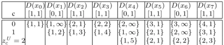
Example 8 Table 1 shows an execution of Algorithm 3 on WEIGHTEDFOCUSfrom
Example 6. Note that |P0| = 5. Hence, zcU = max(zc) − |P0| = 2. As can be seen
from the table, the constraint has a solution as there exists a set S2,7 = {s0,3, s5,7}
such that |S2,7| = 2. D(x0) D(x1) D(x2) D(x3) D(x4) D(x5) D(x6) D(x7) c [1, 1] [0, 1] [1, 1] [1, 1] [0, 1] [1, 1] [0, 1] [1, 1] 0 {1, 1} {1, ∞} {2, 1} {2, 2} {2, ∞} {3, 1} {3, ∞} {4, 1} 1 {1, 2} {1, 3} {1, 4} {1, ∞} {2, 1} {2, ∞} {3, 1} zU c = 2 {1, 5} {2, 1} {2, 2} {2, 3}
Table 1 An execution of Algorithm 3 on WEIGHTEDFOCUSfrom Example 6. Dummy values fc,j are
removed.
Bounds consistency To enforceBCon the sequence [x0, x1, . . . , xn−1], we compute
an additional DP table b, bc,j, c ∈ [0, zcU], j ∈ [−1, n − 1] on the reverse sequence of
variables (i.e. [xn−1, . . . , x1, x0]).
Lemma 11 Consider WEIGHTEDFOCUS(X, yc, len, k , zc). Bounds consistency can
Proof We build dynamic programming tables f and b. We will show that to check if xi = v has a support it is sufficient to examine O(zcU) pairs of values fc1,i−1 and
bc2,n−i−2, c1, c2∈ [0, z
U
c ] which are neighbour columns to the ith column. It is easy
to show that if we consider all possible pairs of elements in fc1,i−1 and bc2,n−i−2
then we determine if there exists a support for xi = v. There are O(zcU × zcU) such
pairs. The main part of the proof shows that it sufficient to consider O(zcU) such
pairs. Next, we provide a formal proof.
Consider dynamic programming tables f and b and a variable-value pair xi = v.
We will show that to check if xi= v has a support it is sufficient to examine O(zcU)
pairs of values fc1,i−1 and bc2,n−i−2, c1, c2 ∈ [0, z
U
c ]. We introduce two dummy
variables x−1and xn, D(x−1) = D(xn) = 0 to keep uniform notations.
Consider a variable-value pair xi = v, v > k. Note that it is sufficient to find a
support one value v, v > k as all values greater than k are indistinguishable. Due to Lemma 10 it is sufficient to consider only elements in the neighbouring columns to the ith column in f and b. Namely, the (i − 1)th column in f and (n − i − 2) in b. The reason for that is that elements in these columns fc1,i−1 and bc2,n−i−2,
c1, c2 ∈ [0, zcU] correspond to sets of sequences, Sc1,i−1 and Sc2,n−i−2, that are
optimal with respect to conditions 1–4 for the prefix [x0, . . . , xj−1] and the suffix
[xj+1, . . . , xn−1], respectively. The main goal is to check whether we can ‘glue’ the
corresponding partial covers Sc1,i−1, Sc2,n−i−2with xi = v into a single cover S
over all variables that satisfies the constraint. To glue Sc1,i−1, Sc2,n−i−2and xi= v
into a single cover we have few options:
– The first and the most expensive option is to create a new sequence s0 of length 1 to cover xi. Then the union S = Sc1,i−1∪ Sc2,n−i−2∪ {s
0} forms a cover s.t.
cst(S) = c1+ c2+ 1 and |S| = |Sc1,i−1| + |Sc2,n−i−2| + 1.
– The second option is to extend last(Sc1,i−1) to the right by one if
|last(Sc1,i−1)| < len. Hence, the updated set S
0
c1,i−1 is identical to Sc1,i−1
except the last sequence is increased by one element on the right. Then the union S = Sc01,i−1 ∪ Sc2,n−i−2 forms a cover: cst(S) = c1 + c2 + 1 and
|S| = |Sc1,i−1| + |Sc2,n−i−2|.
– The third option is to extend last(Sc2,n−i−2) to the left by one if
|last(Sc2,n−i−2)| < len. This case is symmetric to the previous case.
– The fourth and the cheapest option is to glue last(Sc1,i−1), xv and
last(Sc2,n−i−2) to a single sequence if |last(Sc1,i−1)| + |last(Sc2,n−i−2)| <
len. Hence, S0c1,i−1 = Sc1,i−1 \ last(Sc1,i−1), S
0
c2,n−i−2 = Sc2,n−i−2 \
last(Sc2,n−i−2) and s
0 is a concatenation of last(S
c1,i−1), x = v and
last(Sc2,n−i−2)]. Then the union S = S
0
c1,i−1∪ S
0
c2,n−i−2∪ {s
0} forms a cover:
cst(S) = c1+ c2+ 1 and |S| = |Sc1,i−1| + |Sc2,n−i−2| − 1.
We can go over all pairs fc1,i−1 and bc2,n−i−2, c1, c2 ∈ [0, z
U
c ] and check the
four cases above. If obtained cover S is such that cst(S) ≤ zU
c and |S| ≤ max(yc)
then we have found a support for xi= v. Otherwise, xi= v does not have a support
due to Lemma 10. However, if we need to consider all pairs fc1,i−1and bc2,n−i−2,
c1, c2 ∈ [0, zcU] then finding a support takes O((zcU)2) time. We show next that it
is sufficient to consider a linear number of pairs. We observe that in all four options above the cost of resulting cover S is c1+ c2+ 1. Therefore, we only need to consider
pairs fc1,i−1and bc2,n−i−2such that c1+c2+1 ≤ z
U
c . Therefore, for each fc1,i−1it is
sufficient to consider only one element bc2,n−i−2such that bc2,n−i−2is non-dummy
and c2is the maximum value that satisfies inequality c1+ c2+ 1 ≤ zcU.
We prove by contradiction. Suppose, there exists a pair fc1,i−1 and bc02,n−i−2
such that c1+ c02+ 1 ≤ zcU and Sc1,i−1and Sc02,n−i−2can be extended to a support.
However, Sc1,i−1and Sc2,n−i−2can not be extended to a support for xi = v, c1+
c2+ 1 ≤ zcU and c02< c2. By Lemma 9, we know bc0
2,n−i−2≤ bc2,n−i−2. However,
in this case, |Sc1,i−1| + |Sc2,n−i−2| ≤ |Sc1,i−1| + |Sc02,n−i−2| ≤ max(yc) + 1. In
the case of equality, we know that last(Sc2,n−i−2) < last(Sc02,n−i−2). Hence, if
Sc1,i−1and Sc02,n−i−2can be extended to a support then Sc1,i−1and Sc2,n−i−2can
be extended to a support. This leads to a contradiction.
Note that we do not need to search for each fc1,i−1 as we can find its pair
bc2,n−i−2in O(1) due to consecutivity property of non-dummy values in each
col-umn (Lemma 8). Hence, we need O(zcU) = O(max(zc)) time to check for support
for xi= v.
Consider a variable-value pair xi = v, v ≤ k. Note that it is sufficient to find
a support for one value v, v ≤ k as all values less than or equal to k are in-distinguishable. We again consider all pairs in the neighbouring columns, fc1,i−1
and bc2,n−i−2and consider how to ‘glue’ the corresponding partial covers Sc1,i−1,
Sc2,n−i−2 with xi = v into a single cover S over all variables to satisfy the
constraint. In this case, there is only one option to join Sc1,i−1 and Sc2,n−i−2.
Then union S = Sc1,i−1 ∪ Sc2,n−i−2 forms a cover: cst(S) = c1 + c2 and
|S| = |Sc1,i−1| + |Sc2,n−i−2|. We can go over all pairs fc1,i−1 and bc2,n−i−2,
c1, c2 ∈ [0, zcU] to check if such a pair exists. We again show that it is sufficient
to consider a linear number of pairs. We observe that in all four options above the cost of resulting cover S is c1+ c2. Therefore, we only need to consider pairs fc1,i−1
and bc2,n−i−2such that c1+ c2 ≤ z
U
c . Therefore, for each fc1,i−1it is sufficient to
consider only one element bc2,n−i−2such that bc2,n−i−2is non-dummy and c2is the
maximum value that satisfies inequality c1+ c2≤ zcU.
We prove by contradiction. Suppose, there exists a pair fc1,i−1and bc02,n−i−2such
that c1+ c02≤ zcU and Sc1,i−1and Sc02,n−i−2can be extended to a support. However,
Sc1,i−1 and Sc2,n−i−2can not be extended to a support for xi = v, c1+ c2 ≤ z
U c
and c02 < c2. By Lemma 9, we know bc0
2,n−i−2≤ bc2,n−i−2. However, in this case,
|Sc1,i−1| + |Sc2,n−i−2| ≤ |Sc1,i−1| + |Sc02,n−i−2| ≤ max(yc). In the case of equality,
we know that last(Sc2,n−i−2) < last(Sc02,n−i−2). Hence, if Sc1,i−1and Sc02,n−i−2
can be extended to a support then Sc1,i−1and Sc2,n−i−2can be extended to a support.
This leads to a contradiction.
Complexity. We compute the tables f and b. Then we check for a support for two values v1and v2, v1≤ k and v2> k, in D(xi) in O(max(zc)) time for each variable
xi, i = 0, . . . , n − 1. Hence, the time complexity to enforce domain consistency is
O(n max(zc)).
In particular, to check a support for a variable-value pair xi= v, v > k, for each
fc1,i−1 it is sufficient to consider only one element bc2,n−i−2such that bc2,n−i−2is
D(x0) D(x1) D(x2) D(x3) D(x4) D(x5) D(x6) D(x7) c [1, 1] [0, 1] [1, 1] [1, 1] [0, 1] [1, 1] [0, 1] [1, 1] 0 {4, 1} {3, ∞} {3, 2} {3, 1} {2, ∞} {2, 1} {1, ∞} {1, 1} 1 {3, 1} {2, ∞} {2, 2} {2, 1} {1, ∞} {1, 3} {1, 2} zU c = 2 {2, 4} {2, 3} {2, 1} {1, 5} {1, 4}
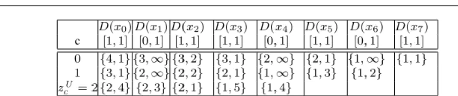
Table 2 An execution of Algorithm 3 on the reverse sequence of variables in WEIGHTEDFOCUSfrom Example 6. Dummy values bc,jare removed.
To check a support for a variable-value pair xi = v, v ≤ k, for each fc1,i−1 it is
sufficient to consider only one element bc2,n−i−2such that bc2,n−i−2is non-dummy
and c2is the maximum value that satisfies inequality c1+ c2≤ zcU. ut
Example 9 Table 2 shows an execution of Algorithm 3 on the reversed sequence of variables x of FOCUSfrom Example 6.
Consider, for example, the variable x4. To check if x4 = 1 has as a support we
need to consider two pairs: f0,3, b1,5and f1,3, b0,5.
Consider the first pair: f0,3 = {2, 2} and b1,5 = {1, 3}. As |S0,3| + |S1,5| =
2 + 1 = max(yc) + 1 = 3, we check whether we can merge last(S0,3), x4= 1, and
last(S1,5). Hence, |last(S0,3)| + |last(S1,5)| = 2 + 3 = len = 5. Therefore, we
cannot merge last(S0,3), xi= 1 and last(S1,5) into a single sequence s0of length 5.
Consider the second pair: f1,3 = {1, 4} and b0,5 = {2, 1}. As |S1,3| + |S0,5| =
1 + 2 = max(yc) + 1 = 3, x4= 1, we check whether we can merge last(S1,3) and
last(S0,5). As |last(S1,3)| + |last(S0,5)| = 4 + 1 is equal to len = 5, we cannot
merge last(S1,3), xi = 1 and last(S0,5) into a single sequence s0 of length at most
5. The second pair cannot be used to build a support for x4= 1. Hence, x4= 1 does
not have a support.
To check if x4= 0 has as support we need to consider pairs: f0,3, b2,5and f1,3,
b1,5. Consider the first pair: f0,3= {2, 2} and b2,5= {2, 1}. We have |S0,3|+|S2,5| =
2 + 2 = max(yc) = 4. Hence, x4= 0 has a support. ut
We observe a useful property of the constraint. If there exists fc,n−1such that
c < max(zc) and qc,n−1< max(yc) then the constraint is BC. This follows from the
observation that given a solution of the constraint SX, changing a variable value can
increase cst(SX) and |SX| by at most one.
Decomposition withO(n) variables and constraints. Alternatively we can decom-pose WEIGHTEDFOCUSusing O(n) additional variables and constraints.
Given FOCUS(X, yc, len, k ), let zc be a variable and B=[b0, b1, . . . , bn−1]
be a set of variables such that ∀ bl ∈ B, D(bl) = {0, 1}. We can decompose
WEIGHTEDFOCUSas follows:
WEIGHTEDFOCUS(X, yc, len, k , zc) ⇔ FOCUS(X, yc, len, k ) ∧ [∀l, 0 ≤ l < n,
[(xl≤ k ) ∧ (bl= 0)] ∨ [(xl> k ) ∧ (bl= 1)]] ∧Pl∈{0,1,...,n−1}bl≤ zc.
Enforcing BC on each constraint of the decomposition is weaker than BC on WEIGHTEDFOCUS. Given xl ∈ X, a value may have a unique support for
FOCUS which violates P
D(x0)=D(x2)={1}, D(x3)={0}, and D(x1)=D(x4)={0, 1}, D(yc) = {2},
D(zc) = {3}, k =0 and len=3. Value 1 for x4corresponds to this case.
Another interesting approach for solving WEIGHTEDFOCUS is to reformulate
it as an integer linear program. If the constructed ILP is tractable as was the case for SPRINGYFOCUS, then we can obtain an alternative filtering algorithm for WEIGHTEDFOCUS. However, the approach that we used in Section 3.3 does not work for WEIGHTEDFOCUS. Recall that in Section 3.3 it was sufficient to consider O(n) possible sequences with distinct starting points. It is essential that sequences have distinct starting points as this ensures that the resulting ILP has the consecutive ones property. By relaxing the disjointness requirement, we used these sequences to find a solution of SPRINGYFOCUSOVERLAPand transform it into a solution of SPRINGYFOCUS. The following example shows that the same approach does not work for WEIGHTEDFOCUS.
Example 10 Consider variables X = [x0, x1, . . . , x5] with domains
[1, {0, 1}, 1, 1, {0, 1}, 1] and WEIGHTEDFOCUS(X, [2, 3], 3, 0, [0, 4]).
Fol-lowing approach in Section 3.3, we consider six sequences So
X =
{s0,2, s1,3, s2,4, s3,5, s4,6, s5,6, s6,6}. The cost of any solution that uses sequences
from So
X is 6. However, there exists a solution of WEIGHTEDFOCUSwith cost 4:
SX = {s0,1, s2,3, s5,5}, yc= 3 and zc= 4.
5 Weighted Springy FOCUS
We consider a further generalization of the FOCUS constraint that combines
SPRINGYFOCUSand WEIGHTEDFOCUS. We prove that we can propagate this con-straint in O(n max(zc)) time, which is same as enforcing BC on WEIGHTEDFOCUS.
5.1 Definition and Filtering Algorithm
Definition 10 Let yc and zc be two variables and k , len, h be three integers, such
that 1 ≤ len ≤ |X| and 0 < h < len − 1. An instantiation of X ∪ {yc} ∪ zcsatisfies
WEIGHTEDSPRINGYFOCUS(X, yc, len, h, k , zc) iff there exists a set SX of disjoint
sequences of indices si,jsuch that five conditions are all satisfied:
1. |SX| ≤ yc
2. ∀xl∈ X, xl> k ⇒ ∃si,j∈ SXsuch that l ∈ si,j
3. ∀si,j∈ SX, |{l ∈ si,j, xl≤ k }| ≤ h
4. ∀si,j∈ SX, j − i + 1 ≤ len, xi > k and xj > k.
5. P
si,j∈SX|si,j| ≤ zc.
We can again partition cost of S into two terms. P
si,j∈S|si,j| =
P
si,j∈Scst(si,j) + |Pk|. However, cst(si,j) is the number of undetermined and
neu-tralvariables covered si,j, cst(si,j) = |{p|xp∈ Uk∪ Nk, xp∈ si,j}| as we allow to
The propagator is again based on a dynamic program that for each prefix of vari-ables [x0, x1, . . . , xj] and given cost c computes a cover Sc,jof minimum cardinality
that covers all penalized variables in the prefix [x0, x1, . . . , xj] and has cost exactly
c. We face the same problem of how to compare two sets Sc,j1 and S 2
c,jof minimum
cardinality. The issue here is how to compare last(S1
c,j) and last(Sc,j2 ) if they cover
a different number of neutral variables. Luckily, we can avoid this problem due to the following monotonicity property. If last(S1
c,j) and last(Sc,j2 ) are not equal to infinity
then they both end at the same position j. Hence, if last(Sc,j1 ) ≤ last(Sc,j2 ) then the number of neutral variables covered by last(S1
c,j) is no larger than the number of
neutral variables covered by last(S2c,j). Therefore, we can define order on sets Sc,j
as we did in Section 4 for WEIGHTEDFOCUS.
Our bounds disentailment detection algorithm for WEIGHTEDSPRINGYFOCUS
mimics Algorithm 3. We show a pseudocode for it in Algorithm 4.
Algorithm 4: WEIGHTEDSPRINGYFOCUS(x0, . . . , xn−1)
1 for c ∈ −1..zU c do 2 for j ∈ −1..n − 1 do 3 fc,j← {∞, ∞, ∞}; 4 f0,−1← {0, 0, 0} ; 5 for j ∈ 0..n − 1 do 6 for c ∈ 0..j do 7 if xj∈ Pkthen /* penalizing */ 8 if (lc,j−1∈ [1, len)) ∨ (qc,j−1= ∞); 9 then 10 fc,j← {qc,j−1, lc,j−1+ 1, hc,j−1}; 11 else 12 fc,j← {qc,j−1+ 1, 1, 0}; 13 if xj∈ Ukthen /* undetermined */ 14 if (lc−1,j−1∈ [1, len) ∧ qc−1,j−1= qc,j−1) ∨ (qc,j−1= ∞); 15 then 16 fc,j← {qc−1,j−1, lc−1,j−1+ 1, hc−1,j−1}; 17 else 18 fc,j← {qc,j−1, ∞, ∞} ; 19 if xj∈ Nkthen /* neutral */ 20 if (lc−1,j−1∈ [1, len) ∧ hc−1,j−1∈ [1, h) ∧ qc−1,j−1= qc,j−1) ∨ (qc,j−1= ∞); 21 then 22 fc,j← {qc−1,j−1, lc−1,j−1+ 1, hc−1,j−1+ 1}; 23 else 24 fc,j← {qc,j−1, ∞, ∞} ; 25 return f ;
We highlight two non-trivial differences between Algorithm 4 and Algorithm 3. The first difference is that each cell in the dynamic programming table fc,j, c ∈
[0, zU
c ], j ∈ {0, 1, . . . , n − 1}, where zcU = max(zc) − |Pk|, is a triple of values
qc,j, lc,jand hc,j, fc,j= {qc,j, lc,j, hc,j}. The new parameter hc,jstores the number
of neutral variables covered by last(Sc,j). The second difference is in the way we

![Fig. 3 The same initial configuration of Figure 1 (A) Problem with 4 fixed activities and one activity of length 5 that can start from time 3 to 5 (i.e., D(st)=[3,5])](https://thumb-eu.123doks.com/thumbv2/123doknet/11300547.281393/15.892.110.611.416.546/initial-configuration-figure-problem-fixed-activities-activity-length.webp)