Cutting planes from two rows of a simplex tableau
K. Andersen
Q. Louveaux
R. Weismantel
L. Wolsey
May 2, 2006
Abstract1
Introduction
In this paper a basic geometric object is investigated that allows us to derive cutting planes for general mixed integer linear programs by considering two rows of a simplex tableau simultaneously. Throughout this paper the mixed integer linear program (MIP) is given in equation form, i.e., the optimization problem is defined for a set I of integer variables, a set C of continuous variables, a rational matrix A, a rational vector b of right hand sides and a rational objective function vector c (of suitable dimensions)
(MIP) max cTx subject to Ax = b, x
≥ 0, xi∈ Z for i ∈ I.
Let LP denote the linear programming relaxation of MIP, i.e., the linear program obtained by replacing the condition xi∈ Z with the weaker condition xi∈ R. In cutting plane theory, the goal
is to determine linear inequalities !i∈I∪Caixi ≥ a0 that satisfy
• every feasible solution x to MIP satisfies!i∈I∪Caixi ≥ a0, and
• a vertex x∗ of LP is cut off by the linear inequality, i.e., !
i∈I∪Caix∗i < a0.
From linear programming theory, it follows that a vertex x∗ of LP corresponds to a basic feasible
solution of a simplex tableau associated with subsets B and N of so-called basic and nonbasic variables
xi+
"
j∈N
¯ai,jxj = ¯bi for i ∈ B.
Any row associated with an index i ∈ B ∩ I such that ¯bi$∈ Z gives rise to a set
X(i) :=#x∈ R|N|| ¯b i−
"
j∈N
¯ai,jxj∈ Z, xj ≥ 0 for all j ∈ N$
whose analysis provides inequalities that are violated by x∗. Indeed, Gomory’s mixed integer cuts
[5] and mixed integer rounding cuts [7] are derived from such a basic set X(i), that is – associated with exactly one index i ∈ B ∩ I such that ¯bi$∈ Z. Interestingly, unlike in the pure integer case,
no finite convergence proof of a cutting plane algorithm is known when Gomory’s mixed integer cuts or mixed integer rounding cuts are applied only. More drastically, in [4], an interesting mixed integer program in three variables is presented, and it is shown that none of the known classes of general cutting planes contain the cut needed to solve this problem.
Example 1: Consider the mixed integer set t≤ x1,
t≤ x2,
x1+ x2+ t ≤ 2,
x∈ Z2and t ∈ R1.
The projection of this set onto the space of x1 and x2 variables is given by {(x1, x2) ∈ R2+ :
x1+ x2≤ 2} and is illustrated in Fig. 1. A simple analysis shows that the inequality x1+ x2≤ 2,
or equivalently t ≤ 0, is valid. In [4] it is, however, shown that with the objective function z = max t, traditional mixed integer cutting plane algorithms do not converge finitely.
In this paper we provide some insight into why cutting plane algorithms based on Gomory’s mixed integer cuts, split cuts, lift-and-project cuts [3] and MIR cuts do not always converge in finite time. Roughly speaking, the reason is that all the traditional cutting planes arise from sets X(i) associated with one integer variable xi.
2
1
2
1
r
2r
1r
30
x1
+ x2
≤ 2
f = (
23.
23)
x
2x1
Figure 1: The Instance in [4]
We go one step further in this paper by considering two indices i1, i2∈ B ∩ I simultaneously.
It turns out that the underlying basic geometric object is significantly more complex than its one-variable counterpart. The set that we denote by X(i1, i2) is described as
X(i1, i2) :=#x∈ R|N|| ¯bi−
"
j∈N
¯ai,jxj ∈ Z for i = i1, i2, xj≥ 0 for all j ∈ N$.
Setting f := %¯bi1, ¯bi2 & ∈ R2, and rj := %¯a i1, ¯ai2 & ∈ R2,
the set obtained from two rows of a simplex tableau can be represented as PI := {(x, s) ∈ Z2× Rn+: x = f +
"
j∈N
sjrj},
where f is fractional and rj ∈ R2for all j ∈ N.
Example 1 (revisited): For the instance of Example 1, introduce slack variables, s1, s2 and y1
in the three constraints. Then, solving as a linear program, the constraints of the optimal simplex tableau are
t +13s1 +13s2 +13y1 = 23
x1 −23s1 +13s2 +13y1 = 23
x2 +13s1 −23s2 +13y1 = 23
Taking the last two rows, and rescaling s$
i = si/3 for i = 1, 2, we obtain the set PI
x1 −2s$1 +1s$2 +13y = + 2 3 x2 +1s$1 −2s$2 +13y = + 2 3 x∈ Z2, s∈ R2 +, y1∈ R1+.
Letting f = (2 3,
2 3)
T, r1 = (2, −1)T, r2 = (−1, 2)T and r
3 = (−13,−13) (see Fig. 1), one easily
obtains the desired cut for conv(PI)
x1+ x2+ y1≥ 2 or equivalently t ≤ 0,
which, when used in a cutting plane algorithm, yields immediate termination.
Our main contribution is to characterize geometrically all the facets of conv(PI). All facets are
intersection cuts [2], i.e., they can be obtained from a (two-dimensional) convex body that does not contain any integer points in its interior. Our geometric approach is based on two important facts that we prove in this paper
• every facet is derivable from at most four nonbasic variables.
• with every facet F one can associate three or four particular vertices of conv(PI). The
classification of F depends on how these k = 3, 4 vertices can be partitioned into k sets of cardinality at most two.
More precisely, the facets of conv(PI) can be distinguished with respect to the number of sets that
contain two integer points. Since k = 3 or k = 4, the following interesting situations occur • no sets with cardinality two: all the k ∈ {3, 4} sets contain exactly one tight integer point.
We call cuts of this type disection cuts.
• exactly one set has cardinality two: in this case we show that the inequality can be derived from lifting a cut associated with a two-variable subproblem to k variables. We call these cuts lifted two-variable cuts.
• two sets have cardinality two. In this case we show that the corresponding cuts are split cuts.
Furthermore, we show that inequalities of the first two families are never split cuts. Our geometric approach allows us to generalize the cut introduced in Example 1. More specifically, the cut of Example 1 is a degenerate case in the sense that it is “almost” a disection cut and “almost” a lifted two-variable cut: by perturbing the vectors r1, r2 and r3 slightly, the cut in Example 1
can become both a disection cut and a lifted two-variable cut.
We review some basic facts about the structure of conv(PI) in Section 2. In Section 3 we explore
the geometry of all the feasible points that are tight for a given facet of conv(PI). Section 4 explains
our main result and presents the classification of all the facets of conv(PI). Finally, Section 5
presents a combinatorial polynomial-time algorithm to compute all the vertices of conv(PI). This
algorithm can be used to construct a polynomial time separation algorithm.
2
Basic structure of conv(P
I)
The basic mixed-integer set considered in this paper isPI := {(x, s) ∈ Z2× Rn+: x = f +
"
j∈N
sjrj}, (1)
where N := {1, 2, . . . , n}, f ∈ Q2\Z2and rj∈ Q2for all j ∈ N. The set P
LP := {(x, s) ∈ R2×Rn+:
x = f +!j∈Nsjrj} denotes the LP relaxation of PI. The jthunit vector in Rn is denoted ej. In
this section, we describe some basic properties of conv(PI). The vectors {rj}j∈N are called rays,
and we assume rj
Lemma 1 The set PI is empty if and only if
(i) All rays {rj
}j∈N are parallel.
(ii) The lines {f + sjrj : sj∈ R} for j ∈ N do not contain any integer points.
Proof: Clearly (i) and (ii) are sufficient. Suppose PI = ∅. If there are j, k ∈ N such that rj and
rk are not parallel, the set f + cone({rj, rk
}) contains integer points. Hence all rays {rj
}j∈N are
parallel, and the sets {f + sjrj : sj ∈ R} for j ∈ N do not contain any integer points.
In the remainder of the paper we assume PI $= ∅. The next lemma gives a characterization of
conv(PI) in terms of vertices and extreme rays.
Lemma 2
(i) The dimension of conv(PI) is n.
(ii) The extreme rays of conv(PI) are (rj, ej) for j ∈ N.
(iii) The vertices (xI, sI) of conv(P
I) take the following two forms:
(a) (xI, sI) = (xI, sI
jej), where xI = f + sIjrj ∈ Z2 and j ∈ N
(an integer point on the ray {f + sjrj : sj≥ 0}).
(b) (xI, sI) = (xI, sI
jej+ sIkek), where xI = f + sIjrj+ sIkrk ∈ Z2 and j, k ∈ N
(an integer point in the set f + cone({rj, rk
})).
Proof: Let (¯x, ¯s) ∈ PI be arbitrary. (ii): For any j ∈ N, since rj ∈ Q2, there exists a positive
integer qj such that qjrjis integer. Hence we have f + !j∈N¯sjrj+ qjrj∈ Z2. This proves (rj, ej)
is a ray of conv(PI) for all j ∈ N. In addition, every other ray of conv(PI) can be expressed as a
conic combination of these rays. (i): The (n + 1) points (¯x, ¯s) and {(¯x + qjrj, ¯s + qjej)}j∈N are
in PI and affinely independent. (iii): If (¯x, ¯s) is a vertex of conv(PI), then ¯x is integer, and ¯s is a
basic solution to the system ¯x = f + !j∈Nsjrj and sj ≥ 0 for all j ∈ N.
Using Lemma 2, we now give a simple form for the valid inequalities for conv(PI) considered
in the remainder of the paper.
Corollary 1 Every non-trivial valid inequality for PI that is tight at a point (¯x, ¯s) ∈ PI can be
written in the form "
j∈N
αjsj ≥ 1, (2)
where αj≥ 0 for all j ∈ N.
Proof: Let !j∈Nαjsj ≥ β be a non-trivial valid inequality for conv(PI), and let (¯x, ¯s) ∈ PI be
a tight feasible point, i.e., !j∈Nαj¯sj = β. Suppose there exists j ∈ N such that αi < 0. From
Lemma 2.(ii), we have (¯x+rj, ¯s+ e
j) ∈ conv(PI), which contradicts the validity of !j∈Nαjsj≥ β
for conv(PI). Hence αj ≥ 0 for all j ∈ N. Since !j∈Nαj¯sj ≥ 0, we can not have β < 0. If
β = 0,!j∈Nαjsj ≥ β is a non-negative combination of the inequalities sj ≥ 0 for j ∈ N, which
contradicts the assumption that !j∈Nαjsj ≥ β is non-trivial.
For an inequality !j∈Nαjsj ≥ 1 of the form (2), let Nα0 := {j ∈ N : αj = 0} denote the
variables with coefficient zero, and let N%=0
α := N \ Nα0 denote the remainder of the variables. We
now introduce an object that is associated with the inequality !j∈Nαjsj ≥ 1. We will use this
Lemma 3 Let !j∈Nαjsj ≥ 1 be a valid inequality for conv(PI) of the form (2). Define vj :=
f +α1jrj for j ∈ N%=0
α . Consider the convex polyhedron in R2
Lα= {x ∈ R2: there exists s ∈ Rn+ s.t. (x, s) ∈ PLP and
" j∈N αjsj≤ 1}. (i) Lα= conv({f} ∪ {vj}j∈N!=0 α )+ cone({r j }j∈N0 α).
(ii) interior(Lα) does not contain any integer points.
(iii) If interior(Lα) $= ∅, then f ∈ interior(Lα).
Proof: (i) First suppose ¯x ∈ Lα. This means there exists ¯s ∈ Rn+ such that !j∈Nαj¯sj ≤ 1
and ¯x = f + !j∈N¯sjrj. Therefore, we may write ¯x = λ0f +!j∈N0 αλjv
j+ !
j∈Nα!=0¯sjr
j, where
λj = ¯sjαj for j ∈ Nα%=0 and λ0 = 1 −!j∈N!=0λj, which shows ¯x ∈ conv({f} ∪ {vj}j∈N!=0 α )+ cone({rj }j∈N0 α). Conversely, if ¯x ∈ conv({f} ∪ {v j }j∈N!=0 α )+ cone({r j }j∈N0 α), then ¯x = λ0f + ! j∈Nα!=0λjv j+ ! j∈N0 αµjr j, where {µ j}j∈N0 α ⊂ R+, λ0≥ 0, {λj}Nα!=0⊂ R+and λ0+!j∈Nλj= 1.
Hence, we may write ¯x = f + !j∈N¯sjrj, where ¯sj = αλjj for j ∈ Nα%=0 and ¯sj = µj for j ∈ Nα0,
and therefore ¯x ∈ Lα. (ii) If ¯x ∈ interior(Lα), then there exists ¯s ∈ Rn+ such that (¯x, ¯s) ∈ PLP
and !j∈Nαj¯sj < 1. Since!j∈Nαjsj≥ 1 is valid for PI, we can not have that ¯x is integer. (iii)
This is clear from the facts that f can be represented using s = 0 and interior(Lα) can be written
in the form {x ∈ R2: ∃s ∈ Rn
+ s.t. (x, s) ∈ PLP and !j∈Nαjsj< 1}.
Example 2: Consider the set PI = {(x, s) ∈ Z2× R5+: x = f + ' 2 1 ( s1+ ' 1 1 ( s2+ ' −3 2 ( s3+ ' 0 −1 ( s4+ ' 1 −2 ( s5}, where f =' 14 1 2 (
, and consider the inequality
2s1+ 2s2+ 4s3+ s4+
12
7 s5≥ 1. (3)
The corresponding set Lαis shown in Fig. 2. As can be seen from the figure, Lαdoes not contain
any integer points in its interior. It follows that (3) is valid for conv(PI). Note that, conversely,
the coefficients αj for j = 1, 2, . . . , 5 can be obtained from the polygon Lα as follows: αj is the
ratio between the length of rj and the distance between f and vj. In particular, if the length of
rj is 1, then α
j is the inverse of the distance from f to vj.
The interior of Lαgives a two-dimensional representation of the points x ∈ R2that are affected
by the addition of the inequality !j∈Nαjsj ≥ 1 to the LP relaxation PLP of PI. In other words,
for any (x, s) ∈ PLP that satisfies !j∈Nαjsj < 1, we have x∈ interior(Lα). Furthermore, for a
facet defining inequality !j∈Nαjsj ≥ 1 of conv(PI), there exists n affinely independent points
(xi, si) ∈ P
I, i = 1, 2, . . . , n, such that !j∈Nαjsij = 1. The integer points {xi}i∈N are on the
boundary of Lα, i.e., they belong to the following integer set:
Xα:= {x ∈ Z2: ∃s ∈ Rn+ s.t. (x, s) ∈ PLP and
"
j∈N
αjsj= 1}.
We have Xα= Lα∩ Z2, and Xα$= ∅ whenever!j∈Nαjsj≥ 1 defines a facet of conv(PI). In
Sect. 3 we characterize conv(Xα). This characterization is then used in Sect. 4 to characterize
r
1r
2r
3r
4r
5v
1v
2v
3v
4v
5Lemma 4 Any facet defining inequality !j∈Nαjsj ≥ 1 for conv(PI) of the form (2) that has
some zero coefficients is a split cut. In other words, if N0
α$= ∅, there exists (π, π0) ∈ Z2× Z such
that Lα⊆ {(x1, x2) : π0≤ π1x1+ π2x2≤ π0+ 1}.
Proof: Let k ∈ N0
α be arbitrary. Then the line {f + µrk : µ ∈ R} does not contain any
in-teger points. Furthermore, if j ∈ N0
α, j $= k, is such that rk and rj are not parallel, then
f + cone({rk, rj
}) contains integer points. It follows that all rays {rj
}j∈N0
αare parallel. By letting
π$ := (rk)⊥ = (−rk 2 rk 1 ) and π $ 0:= (π$)Tf , we have {f + µrk : µ ∈ R} = {(xx12) : π $ 1x1+ π$2x2= π0$}. Now define: π1
0 := max{π$1x1+ π2$x2: π1$x1+ π2$x2≤ π0$ and x ∈ Z2}, and
π02:= min{π$1x1+ π2$x2: π1$x1+ π2$x2≥ π0$ and x ∈ Z2}.
We have π1
0 < π$0 < π02, and the set Sπ := {x ∈ R2 : π01 ≤ π1$x1+ π2$x2 ≤ π02} does not
contain any integer points in its interior. We now show Lα ⊆ Sπ by showing that every vertex
vm= f + 1 αmr
mof L
α, where m ∈ Nα%=0, satisfies vm∈ Sπ. Suppose vmsatisfies π1$v1m+π$2vm2 < π01
(the case π$
1vm1 + π$2vm2 > π02 is symmetric). By definition of π01, there exists xI ∈ Z2 such that
π$
1xI1+ π$2xI2= π01, and xI = λvm+ (1 − λ)(f + δrk), where λ ∈]0, 1[, for some δ > 0. We then have
xI = f + λ αmr
m+ δ(1−λ)rk. Inserting this representation of xI into the inequality !
j∈Nαjsj≥ 1
then gives αmαλm+ αkδ(1− λ) = λ < 1, which contradicts the validity of!j∈Nαjsj ≥ 1 for PI.
Hence Lα⊆ Sπ.
To finish the proof, we show that we may write Sπ = {x ∈ R2: π0≤ π1x1+ π2x2≤ π0+ 1} for
some (π, π0) ∈ Z2×Z. First observe that we can assume (by scaling) that π$, π01and π20are integers.
Next observe that any common divisor of π$
1and π2$ also divides both π01and π20(this follows from
the fact that there exists x1, x2
∈ Z2 such that π$
1x11+ π$2x12= π01 and π$1x21+ π$2x22= π20). Hence
we can assume that π$
1and π2$ are relative prime. Now the Integral Farkas Lemma (see [9]) implies
that the set {x ∈ Z2 : π$
1x1+ π2$x2= 1} is non-empty. It follows that we must have π02= π01+ 1,
since otherwise the point ¯y := x$ + x1
∈ Z2, where x$ ∈ {x ∈ Z2 : π$
1x1 + π2$x2 = 1} and
x1
∈ {x ∈ Z2 : π$
1x1+ π$2x2 = π10}, satisfies π01 < π$1¯y1+ π2$¯y2 < π02, which contradicts that Sπ
does not contain any integer points in its interior.
3
A characterization of conv(X
α)
As a preliminary step of our analysis, we first characterize the set conv(Xα). We assume αj > 0
for all j ∈ N. Clearly conv(Xα) is a convex polygon with only integer vertices, and since Xα⊆ Lα,
conv(Xα) does not have any integer points in its interior. We first limit the number of vertices of
conv(Xα) to four.
Lemma 5 Let P ⊂ R2 be a convex polygon with integer vertices that has no integer points in its
interior.
(i) P has at most four vertices
(ii) If P has four vertices, then at least two of its four facets are parallel.
(iii) If P is not a triangle with integer points in the interior of all three facets (see Fig. 4.(c)), then there exists parallel lines πx = π0 and πx = π0+ 1, (π, π0) ∈ Z3, such that P is
contained in the corresponding split set, i.e., P ⊆ {x ∈ R2: π
0≤ πx ≤ π0+ 1}.
Proof: (i)-(ii): Let v1, v2, . . . , vp denote the vertices of P . Wlog assume v1= 0, and that v2 and
v3 are such that P ⊂ cone(v2, v3). Observe that cone(v2, v3) can be written as the disjoint union
Πi,j:= {z ∈ R2: z = (i + λ2)v2+ (j + λ3)v3, where λ2, λ3∈ [0, 1[},
where i, j ≥ 0. The parallelograms Πi,jare illustrated in Fig. 3. Note that the following translation
property holds: for any integer point wi,j in parallelogram Πi,j, there is a corresponding integer
point wi",j" in parallelogram Πi",j" at the same position. Specifically, if the point wi,j= (i+λ2)v2+
(j + λ3)v3= (iv2+ jv3) + (λ2v2+ λ3v3) ∈ Πi,jis integer, then λ2v2+ λ3v3is integer, and therefore
wi",j" := (i$v2+ j$v3) + (λ2v2+ λ3v3) = (i$+ λ2)v2+ (j$+ λ3)v3∈ Πi",j" is integer (see Fig. 3).
We first claim that every vertex vk, k ≥ 4, must be either on the line L2= {v2+ λv3|λ > 0},
or on the line L3= {λv2+ v3|λ > 0}. First suppose vk ∈ Πi,j, where i, j ≥ 1. Then either vk ∈ L2
or vk∈ L3, since otherwise the integer point v2+ v3 is an interior point of P .
Now suppose vk ∈ Π0,j, where j ≥ 1 (the case when vk ∈ Πi,0, i ≥ 1, is symmetric). This
means there exists λ2, λ3 ∈ [0, 1[ such that vk = λ2v2+ (j + λ3)v3. If λ2 = 0, v3 is on the line
between v1 and vk, which is a contradiction, so we have λ2 > 0. From the translation property
discussed above, we have w := λ2v2+ (j − 1 + λ3)v3 ∈ Z2. We claim w is in the interior of P .
Indeed, we may write
w = j− 1 + λ3 j + λ3 vk+ λ2 j + λ3 v2,
where µ2:=j+λλ23 ∈]0, 1[ and µk:= j−1+λj+λ33 ∈]0, 1[. Hence we have w = µ2v2+µkvk+(1−µ2−µk)v1,
where µ2+ µk = (j+λ3j+λ)−(1−λ3 2) ∈]0, 1[, and this shows w is in the interior of P .
Finally suppose vk ∈ Π0,0. We may therefore write vk = λ2v2+ λ3v3, where λ2, λ3∈ [0, 1[. If
λ2 = 0, vk is on the line between v1 and v3, and if λ3 = 0, vk is on the line between v1 and v2,
so we can assume λ2, λ3 > 0. If λ2+ λ3 < 1, then vk is in the interior of conv({v1, v2, v3}), and
if λ2+ λ3 = 1, vk can not be a vertex. Finally, if λ2+ λ3 > 1, the point w := (v2+ v3) − vk =
(1 − λ2)v2+ (1 − λ3)v3is integer and in the interior of conv({v1, v2, v3}). It follows that vk must
be either in L2 or L3.
To finish the proof of (i) and (ii), we only need to argue that L2∪ L3 can only contain one
vertex of P . Clearly L2 and L3 can only contain one vertex each, so we may assume p = 5,
v4 = v2 + λ3v3 ∈ L2 and v5 = v3+ λ2v2 ∈ L3. Furthermore, we have either λ2, λ3 > 1 or
λ2, λ3 < 1, since otherwise either v4 is in the interior of conv({v1, v2, v3, v5}), or v5 is in the
interior of conv({v1, v2, v3, v4}). If λ2, λ3 > 1, the point v2+ v3 is in the interior of P , and if
λ2, λ3< 1, the point w := λ2v2+ λ3v3 is integer and in the interior of P .
(iii) Consider again the parallelogram Π0,0. If | det(v2, v3)| = 1, it is well known that the vertex
0 is the only integer point contained in Π0,0. Hence all parallelograms Πi,jdo not have any integer
point in their interior. In particular ∪j∈ZΠ0,j and ∪i∈ZΠi,0 do not have any integer point in their
interior. Furthermore P is always contained in at least one of these two sets since a potential vertex v4would be either in L2 or in L3.
Now suppose | det(v2, v3)| > 1. Therefore Π
0,0 contains more than one integer point. If P is a
quadrangle, observe that these points must be on the boundary of Π0,0, since otherwise P would
contain integer points in its interior. If P is a triangle, we assume that the edge (v2, v3) does not
contain an integer point in its interior. Otherwise we can re-index the vertices so that this holds. In this case, it is also true that the integer points of Π0,0 are on its boundary. We claim that all
integer points of Π0,0 must be on the same side of Π0,0, i.e., either in S2:= {λv2: 0 ≤ λ < 1}, or
in S3:= {λv3: 0 ≤ λ < 1}. Suppose we have w2= λ2v2∈ Z2with 0 < λ2< 1 and w3= λ3v3∈ Z2
with 0 < λ3 < 1. Note that λ2 and λ3 can be chosen in ]0, 1/2] by possibly considering v2− w2
or v3− w3, which are also integer. Therefore w2+ w3= λ2v2+ λ3v3 is integer and in the interior
of P if P is a quadrangle. This contradicts the hypothesis that the edge (v2, v3) does not contain
an integer point if it is a triangle. Hence either S2 or S3 does not contain any integer point. This
implies that either ∪j∈ZΠ0,j or ∪i∈ZΠi,0 does not contain an integer point in its interior.
From the proof of Lemma 5, it follows that the polygons in Fig. 4 include all possible polygons that can be included in the set Lα in the case when Lα is bounded and of dimension 2. The
dashed lines in Fig. 4 indicate the possible split sets that include P . We excluded from Fig. 4 the cases when Xα is of dimension 1. We note that Lemma 5.(iii) (existence of split sets) proves
that there cannot be any triangles where two facets have interior integer points, and also that no quadrangle can have more than two facets that have integer points in the interior.
0 v3 v2
L2
L3
w0,2 w1,2 w2,2 w0,1 w1,1 w2,1 w0,0 w1,0 w2,0Π0,2
Π1,2
Π2,2
Π2,1
Π1,1
Π0,1
Π0,0
Π1,0
Π2,0
Figure 3: Partitioning of cone(v2, v3) into parallelograms
4
A characterization of the facets of conv(P
I)
In this section we focus on the set Lα. As in the previous section, we assume αj > 0 for all
j ∈ N. Due to the direct correspondence between the set Lα and a facet defining inequality
!
j∈Nαjsj ≥ 1 for conv(PI), this gives a characterization of the facets of conv(PI). The main
result in this section is that Lαcan have at most four vertices. In other words, we prove
Theorem 2 Let !j∈Nαjsj ≥ 1 be a facet defining inequality for conv(PI) that satisfies αj > 0
for all j ∈ N. Then Lα is a polygon with at most four vertices.
Theorem 2 shows that there exists a set S ⊆ N such that |S| ≤ 4 and !j∈Sαjsj ≥ 1 is facet
defining for conv(PI(S)), where
PI(S) := {(x, s) ∈ Z2× R|S|+ : x = f +
"
j∈S
sjrj}.
Throughout this section we assume that no two rays point in the same direction. If two variables j1, j2 ∈ N are such that j1 $= j2 and rj1 = δrj2 for some δ > 0, then the halflines
{x ∈ R2: x = f + s
j1rj1, sj1 ≥ 0} and {x ∈ R2: x = f + sj2rj2, sj2 ≥ 0} intersect the boundary of
Lαat the same point, and therefore Lα= conv({f}∪{vj}j∈N) = conv({f}∪{vj}j∈N\{j2}), where
vj:= f + 1 αjr
j for j ∈ N. This assumption does therefore not effect the validity of Theorem 2.
The proof of Theorem 2 is based on characterizing the vertices conv(PI) that are tight for
!
(a) A triangle: no facet has in-terior integer points
(b) A triangle: one facet has interior integer points
(c) A triangle: all facets have interior integer points
(d) A quadrangle: no facet has interior integer points
(e) A quadrangle: one facet has interior integer points
(f) A quadrangle: two facets have interior integer points
Figure 4: All integer polygons that do not have interior integer points
of conv(PI) that satisfy !j∈Nαjsj ≥ 1 with equality. In the remainder of this section, the set
{(yi, ti)}
i∈M ⊆ PI denotes n such points, where M := {1, 2, . . . , n}. In other words we have
"
j∈N
αjtij= 1, for i ∈ M. (4)
Since !j∈Nαjsj≥ 1 is facet defining for conv(PI), the values {αj}j∈Nare the unique solution
to (4). It follows that every variable j ∈ N is involved in system (4). We will show that there exists a subset S ⊆ N of variables and a set of |S| affinely independent vertices of conv(PI) such
that |S| ≤ 4 and {αj}j∈S is the unique solution to the equality system defined by these vertices.
Observe that the set {yi}
i∈M is the set of vertices of conv(Xα). We can therefore partition the
equalities (4) according to which vertex of conv(Xα) is involved in each equality. The following
notation will be used intensively in the remainder of this section. Notation 1
(i) The number k ≤ 4 denotes the number of vertices of conv(Xα).
(ii) The set {xv}
v∈K denotes the vertices of conv(Xα), where K := {1, 2, . . . , k}.
(iii) For every v ∈ K, the set Mv := {i ∈ M : yi = xv}, denotes the equalities of (4) for which
xv is the vertex of conv(X
α) involved in the corresponding equality of (4).
The system (4) can now be rewritten as "
j∈N
Lemma 2.(iii) demonstrates that for a vertex (¯x, ¯s) of conv(PI), ¯s is positive on at most two
coordinates j1, j2∈ N, and ¯x ∈ f + cone({rj1, rj2}). If for some i ∈ M, ti is positive on only one
coordinate, then yi= f + ti
jrj for some j ∈ N, and the system (5) includes the equality αjtij= 1,
which simply states αj =t1i
j. A point ¯x ∈ Z
2that satisfies ¯x ∈ {x ∈ R2: x = f + s
jrj, sj≥ 0} for
some j ∈ N will be called a ray point in the remainder of the paper. In order to characterize the equalities of (5) that correspond to vertices xv of conv(X
α) that are not ray points, we introduce
the following concepts.
Definition 1 Let !j∈Nαjsj ≥ 1 be valid for conv(PI). Suppose ¯x ∈ Z2 is not a ray point,
and that ¯x ∈ f + cone({rj1, rj2}), where j
1, j2∈ N. This implies ¯x = f + sj1rj1 + sj2rj2, where
sj1, sj1 > 0 are unique.
(a) The pair (j1, j2) is said to give a representation of ¯x.
(b) If αj1sj1+αj2sj2 = 1, (j1, j2) is said to give a tight representation of ¯x wrt. !j∈Nαjsj ≥ 1.
(c) If (i1, i2) ∈ N × N satisfies cone({ri1, ri2}) ⊆ cone({rj1, rj2}), the pair (i1, i2) is said to
define a subcone of (j1, j2).
Example 2 (continued): Consider again the set
PI = {(x, s) ∈ Z2× R5+: x = f + ' 2 1 ( s1+ ' 1 1 ( s2+ ' −3 2 ( s3+ ' 0 −1 ( s4+ ' 1 −2 ( s5}, where f =' 14 1 2 (
, and the valid inequality 2s1+ 2s2+ 4s3+ s4+127s5 ≥ 1 for conv(PI). The
point ¯x = (1, 1) is on the boundary of Lα (see Fig. 2). We have that ¯x can be written in any of
the following forms
¯x =f+1 4r1+ 1 4r2, ¯x =f+3 7r1 + 1 28r3, ¯x =f + 3 4r2 + 1 4r4.
It follows that (1, 2), (1, 3) and (2, 4) all give representations of ¯x. Note that (1, 2) and (1, 3) give tight representations of ¯x wrt. the inequality 2s1+ 2s2+ 4s3+ s4+127s5≥ 1, whereas (2, 4)
does not. Finally note that (1, 5) defines a subcone of (2, 4). Observe that, for a vertex xv of conv(X
α) and an equality i ∈ Mv, if ti has support two, the
equality !j∈Nαjtij = 1 of system (5) can be written as αj1tji1 + αj2tij2 = 1, where j1, j2 ∈ N
satisfy ti j1, t
i
j2 > 0. Hence, the equality
!
j∈Nαjtij = 1 corresponds to the tight representation
(j1, j2) of xv wrt. !j∈Nαjsj ≥ 1. Furthermore, if ti is positive on only one coordinate, then xv
is a ray point. We now characterize the set of tight representations of an arbitrary integer point ¯x ∈ Z2, which is not a ray point
Tα(¯x) := {(j1, j2) ∈ N × N : (j1, j2) gives a tight representation of ¯x wrt.
"
j∈N
αjsj≥ 1}.
We will show (Lemma 6 and Lemma 7) that Tα(¯x) contains a unique maximal representation
(jx¯
(i) Every subcone (j1, j2) of (j1x¯, j2x¯) that gives a representation of ¯x satisfies (j1, j2) ∈ Tα(¯x).
(ii) Conversely, every (j1, j2) ∈ Tα(¯x) defines a subcone of (j1x¯, j2¯x).
We then use the maximal representations of the vertices of conv(Xα) to rewrite (5) (Lemma
8). From this system, we construct a subset S of variables such that |S| = k and!j∈Sαjsj ≥ 1
is facet defining for conv(PI(S)).
To prove (i) and (ii), there are two cases to consider. For two representations (i1, i2) and
(j1, j2) of ¯x, either one of the two cones (i1, i2) and (j1, j2) is contained in the other, or their
intersection defines a subcone of both (i1, i2) and (j1, j2) (note that we cannot have that their
intersection is empty, since they both give a representation of ¯x). We first consider the case when one cone defines a subcone of another cone.
Lemma 6 Let !j∈Nαjsj ≥ 1 be a facet defining inequality for conv(PI) that satisfies αj > 0 for
all j ∈ N, and let ¯x ∈ Z2. Then (j
1, j2) ∈ Tα(¯x) implies (i1, i2) ∈ Tα(¯x) for every subcone (i1, i2)
of (j1, j2) that gives a representation of ¯x.
Proof: Suppose (j1, j2) ∈ Tα(¯x). Observe that it suffices to prove the following: for any j3 ∈ N
such that rj3 ∈ cone({rj1, rj2}) and (j
1, j3) gives a representation of ¯x, the representation (j1, j3) is
tight wrt. !j∈Nαjsj ≥ 1. The result for all remaining subcones of (j1, j2) follows from repeated
application of this result. For simplicity we assume j1= 1, j2= 2 and j3= 3.
Since ¯x ∈ f + cone({r1, r2 }), ¯x ∈ f + cone({r1, r3 }) and r3 ∈ cone({r1, r2 }), we may write ¯x = f + u1r1+ u2r2, ¯x = f + v1r1+ v3r3 and r3 = w1r1+ w2r2, where u1, u2, v1, v3, w1, w2 ≥
0. Furthermore, since (1, 2) gives a tight representation of ¯x wrt. !j∈Nαjsj ≥ 1, we have
α1u1+ α2u2 = 1. Finally we have α1v1+ α3v3≥ 1, since !j∈Nαjsj ≥ 1 is valid for PI. If also
α1v1+ α3v3= 1, we are done, so suppose α1v1+ α3v3> 1.
We first argue that this implies α3> α1w1+α2w2. Since ¯x = f +u1r1+u2r2= f +v1r1+v3r3,
it follows that (u1− v1)r1= v3r3− u2r2. Now, using the representation r3= w1r1+ w2r2, we get
(u1− v1− v3w1)r1+ (u2− v3w2)r2= 0. Since r1 and r2 are linearly independent, we obtain:
(u1− v1) = v3w1 and u2= v3w2.
Now we have α1v1+ α3v3 > 1 = α1u1+ α2u2, which implies (v1− u1)α1− α2u2+ α3v3 >
0. Using the identities derived above, we get −v3w1α1− α2v3w2+ α3v3 > 0, or equivalently
v3(−w1α1− α2w2+ α3) > 0. It follows that α3> α1w1+ α2w2.
We now derive a contradiction to the identity α3> α1w1+α2w2. Since !j∈Nαjsj≥ 1 defines
a facet of conv(PI), there must exist x$∈ Z2and k ∈ N such that (3, k) gives a tight representation
of x$ wrt. !
j∈Nαjsj ≥ 1. In other words, there exists x$ ∈ Z2, k ∈ N and δ3, δk ≥ 0 such that
x$ = f + δ3r3+ δkrk and α3δ3+ αkδk= 1. Furthermore, we can choose x$, δ3 and δk such that r3
is used in the representation of x$, i.e., we can assume δ 3> 0.
Now, using the representation r3 = w
1r1+ w2r2 then gives x$ = f + δ3r3+ δkrk = f +
δ3w1r1 + δ3w2r2 + δkrk. Since !j∈Nαjsj ≥ 1 is valid for PI, we have α1δ3w1+ α2δ3w2+
αkδk≥ 1 = α3δ3+αkδk. This implies δ3(α3−α1w1−α2w2) ≤ 0, and therefore α3≤ α1w1−α2w2,
which is a contradiction.
To finish the proof of (i) and (ii), we need to consider the case of two cones (j1, j2), (j3, j4) ∈
Tα(¯x), where neither of the two cones is a subcone of the other cone. This case is captured in the
following lemma.
Lemma 7 Let !j∈Nαjsj ≥ 1 be a facet defining inequality for conv(PI) satisfying αj > 0
for j ∈ N, and suppose ¯x ∈ Z2 is not a ray point. Also suppose the intersection between the
cones (j1, j2), (j3, j4) ∈ Tα(¯x) is given by the subcone (j2, j3) of both (j1, j2) and (j3, j4). Then
Proof: For simplicity assume j1 = 1, j2= 2, j3= 3 and j4 = 4. Since the cones (1, 2) and (3, 4)
intersect in the subcone (2, 3), we have r3
∈ cone({r1, r2 }), r2 ∈ cone({r3, r4 }), r4 / ∈ cone({r1, r2 }) and r1 ∈ cone({r/ 3, r4}). We first represent ¯x in the translated cones in which we have a tight
representation of ¯x. In other words, we can write
¯x = f + u1r1+ u2r2, (6)
¯x = f + v3r3+ v4r4 and (7)
¯x = f + z2r2+ z3r3, (8)
where u1, u2, v3, v4, z2, z3> 0. Note that Lemma 6 proves that (8) gives a tight represention of ¯x.
Using (6)-(8), we obtain the relation
% T1,1I2 T1,2I2 T2,1I2 T2,2I2 &% r2 r3 &=% u1r1 v4r4 & , (9)
where T is the 2 × 2 matrix T := % T1,1 T1,2
T2,1 T2,2
&=% (z2− u2) z3
z2 (z3− v3)
& and I
2 is the 2 × 2
identity matrix. On the other hand, the tightness of the representations (6)-(8) leads to the following identities
α1u1+α2u2= 1, (10)
α3v3+α4v4= 1 and (11)
α2z2+α4z3= 1, (12)
where, again, the last identity follows from Lemma 6. Using (10)-(12), we obtain the relation % T1,1 T1,2 T2,1 T2,2 &% α2 α3 &=% u1α1 v4α4 & . (13)
We now argue that T is non-singular. Suppose, for a contradiction, that T1,1T2,2 = T1,2T2,1.
From (7) and (8) we obtain v4r4 = (z3 − v3)r3 + z2r2, which implies z3 < v3, since r4 ∈/
cone({r1, r2
}) ⊇ cone({r2, r3
}). Multiplying the first equation of (13) with T2,2gives T2,2T1,1α2+
T2,2T1,2α3= u1T2,2α1, which implies T1,2(T2,1α2+ T2,2α3) = u1T2,2α1. By using the definition of
T , this can be rewritten as z3(α2z2+ (z3− v3)α3) = u1α1(z3− v3). Since z2α2+ z3α3 = 1, this
implies z3(1 −v3α3) = u1α1(z3− v3). However, from (11) we have v3α3∈]0, 1[, so z3(1 −v3α3) > 0
and u1α1(z3− v3) < 0, which is a contradiction. Hence T is non-singular.
We now solve (9) for an expression of r2 and r3 in terms of r1 and r4. The inverse of the
coefficient matrix on the left hand side of (9) is given by % T1,1−1I2 T1,2−1I2
T2,1−1I2 T2,2−1I2
&, where T−1 := % T−1
1,1 T1,2−1
T2,1−1 T2,2−1
&denotes the inverse of T . We therefore obtain
r2= λ1r1+ λ4r4 and (14)
r3= µ1r1+ µ4r4, (15)
where λ1:= u1T1,1−1, λ4:= v4T1,2−1, µ1:= u1T2,1−1and µ4:= v4T2,2−1. Similarly, solving (13) to express
α2and α3in terms of α1 and α4gives
α2= λ1α1+ λ4α4 and (16)
Now, using for instance (6) and (14), we obtain ¯x = f + (u1+ u2λ1)r1+ (u2λ4)r4, and:
(u1+ u2λ1)α1+ (u2λ4)α4 = (using (10))
(1 − u2α2) + u2λ1α1+ (u2λ4)α4 =
1 + u2(λ1α1+ λ4α4− α2) = 1. (using (16))
To finish the proof, we only need to argue that we indeed have ¯x ∈ f + cone({r1, r4
}), i.e., that ¯x = f + δ1r1+ δ4r4 with δ1= u1+ u2λ1 and δ4 = u2λ4 satisfying δ1, δ4≥ 0. If δ1≤ 0 and
δ4> 0, we have ¯x = f + δ1r1+ δ4r4= f + u1r1+ u2r2, which means δ4r4= (u1− δ1)r1+ u2r2∈
cone({r1, r2
}), which is a contradiction. Similarly, if δ1 > 0 and δ4≤ 0, we have ¯x = f + δ1r1+
δ4r4 = f + v3r3+ v4r4, which implies δ1r1 = v3r3+ (v4− δ4)r4 ∈ cone({r3, r4}), which is also a
contradiction. Hence we can assume δ1, δ4≤ 0. However, since δ1= u1+ u2λ1and δ4= u2λ4, this
implies λ1, λ4 ≤ 0, and this contradicts what was shown above, namely that the representation
¯x = f + δ1r1+ δ4r4satisfies α1δ1+ α4δ4= 1.
By using Lemma 6 and Lemma 7, i.e., the characterization of the tight representations of an integer point, we now rewrite the subsystems of (5) that correspond to vertices xv of conv(X
α)
that satisfy |Mv
| > 1.
Lemma 8 Let !j∈Nαjsj ≥ 1 be a facet defining inequality for conv(PI) s.t. αj > 0 for j ∈ N.
Consider a vertex xv of conv(X
α) that satisfies |Mv| > 1, and the subsystem of (5) corresponding
to xv
"
j∈N
αjtij = 1, for every i ∈ Mv. (18)
Let Jv := {j ∈ N : ti
j > 0 for some i∈ Mv} denote the variables that appear in (18). There exist
two variables jv
1, j2v∈ Jv such that
(i) (jv
1, j2v) gives a tight representation of xv wrt. !j∈Nαjsj≥ 1, i.e., there exists wjv
1, wj2v > 0 such that xv = f + w jv 1r j1v+ wjv 2r jv2 and wjv 1αjv1 + wj2vαjv2 = 1.
(ii) For every j ∈ Jv\ {jv
1, j2v}, we have rj ∈ cone(rj
v
1, rjv2), i.e., there exists wj
1, w j 2 > 0 such that rj = wj 1rj v 1 + wj 2rj v 2.
(iii) {αj}j∈N is the unique solution to the system (5’) obtained from (5) by replacing (18) with
wjv 1αjv1 + wj2vαjv2 = 1, (19) αj= wj1αjv 1 + w j 2αjv 2, for every j ∈ J v \ {jv 1, j2v}. (20)
Proof: Observe that, since |Mv| > 1, there exists i ∈ Mv such that ti is non-zero on two
coordi-nates. Wlog suppose this is true for all i ∈ Mv. For every i ∈ Mv, let ji
1, ji2∈ Jv be such that tiji 1, t i ji 2 > 0. Then (j i
1, j2i) gives a tight representation of xvwrt. !j∈Nαjsj≥ 1 for every i ∈ Mv.
It follows from Lemma 6 and Lemma 7 that there exists jv
1, j2v ∈ Jv such that j1v $= j2v, (j1v, j2v)
gives a tight representation of xv wrt. !
j∈Nαjsj ≥ 1, and (j1i, j2i) defines a subcone of (j1v, j2v)
for all i ∈ Mv. This shows (i) and (ii).
We now show (iii). Clearly equality (19) is implied by (5), since (jv
1, j2v) gives a tight
rep-resentation of xv wrt. !
j∈Nαjsj ≥ 1 (note that (19) might not be part of the system (5)).
Now consider a variable j ∈ Jv
\ {jv
1, j2v}, and define the point x$ := f +wj 1 1αjv1+wj2αjv2r
j on the
halfline {f + sjrj : sj ≥ 0}. By using (ii), we obtain x$ = f+ w
j 1 wj 1αjv1+wj2αjv2r jv 1+ w j 2 wj 1αjv1+wj2αjv2r jv 2.
Inserting this representation of x$into ! j∈Nαjsj≥ 1 then gives w1jαjv1 wj1αjv1+w j 2αjv2 + wj2αjv2 wj1αjv1+w j 2αjv2 = 1. This shows x$ is on the boundary of L
α, and since the intersection point between the halfline
{f + sjrj: sj≥ 0} and the boundary of Lαis unique, we have x$= vj = f +α1jrj, which implies
αj= w1jαjv 1 + w
j 2αjv
2. Hence the system (19)-(20) is implied by (5).
We now show the converse, i.e., that {αj}j∈N is the unique solution to the system (5’) obtained
from (5) by replacing (18) with (19)-(20). Therefore let i ∈ Mv be arbitrary, and let (j
1, j2) :=
(ji
1, ji2) for simplicity. We need to show tij1αj1+ tij2αj2 = 1, where xv= f + tij1r
j1 + ti j2r j2. From (19)-(20) we know αj1 = w j1 1 αjv 1+w j1 2 αjv 2, αj2 = w j2 1αjv 1+w j2 2 αjv 2 and αjv1wjv1+αj2vwj2v = 1, where rj1 = wj1 1 rj v 1+wj1 2 rj v 2, rj2 = wj2 1 rj v 1+wj2 2 rj v 2 and xv= f +wjv 1r jv 1+wjv 2r jv
2. Inserting the expressions
for rj1 and rj2 into the identity xv= f + ti j1r j1+ ti j2r j2 then gives xv= f + (ti j1w j1 1 + tij2w j2 1 )rj v 1+ (ti j1w j1 2 +tij2w j2 2 )rj v
2. Since the representation of xv in the set f +cone(rjv1, rj2v) is unique, it follows
that wjv 1 = t i j1w j1 1 +tij2w j2 1 and wjv 2 = t i j1w j1 2 +tij2w j2
2 . Now, from the equality αjv
1wj1v+αjv2wj2v = 1, we get 1 = αjv 1(t i j1w j1 1 +tij2w j2 1 )+ αjv 2(t i j1w j1 2 +tij2w j2 2 ) = tij1(w j1 1 αjv 1+w j1 2 αjv 2)+ t i j2(w j2 1 αjv 1+w j2 2 αjv 2). Since αj1 = w j1 1 αjv 1 + w j1 2 αjv 2 and αj2= w j2 1 αjv 1 + w j2 2 αjv 2, we obtain t i j1αj1+ tij2αj2 = 1.
By using Lemma 8, we are now able to finish the proof of Theorem 2.
Lemma 9 Suppose !j∈Nαjsj ≥ 1 is facet defining for conv(PI) and αj > 0 for j∈ N. Choose
a set S ⊆ N of variables as follows. Initialize S = ∅, and for every vertex xv of conv(X α):
(i) If Mv= {¯i}, update S := S ∪ Jv, where Jv := {j ∈ N : t¯i
j > 0} denotes the (at most two)
variables appearing in equality ¯i of system (5). (ii) If |Mv
| > 1, update S := S ∪ {jv
1, jv2}, where (j1v, jv2) denotes the tight representation of xv
given in Lemma 8.
Then the inequality !j∈Sαjsj ≥ 1 is facet defining for PI(S), |S| = k and we have Lα =
conv({f} ∪ {vj
}j∈S), where vj = f +α1j for j ∈ S.
Proof: From Lemma 8 and the fact that !j∈Nαjsj ≥ 1 is facet defining for conv(PI), we know
that {αj}j∈N is the unique solution to the system
"
j∈N
αjt¯ij= 1, for all v ∈ K s.t. Mv= {¯i}, (21)
wjv 1αj1v + wj2vαj2v = 1, for all v ∈ K s.t. |M v | > 1, (22) w1jαjv 1 + w j 2αjv 2 = αj, for all v∈ K s.t. |M v | > 1 and j ∈ Jv\ {j1v, j2v}, (23)
Observe that, for a vertex xv of conv(X
α) such that |Mv| > 1 and a variable j ∈ Jv\ {j1v, j2v},
αj only appears in system (23). It follows that {αj}j∈S is the unique solution to the subsystem
(21)-(22) of (21)-(23). Now, since the system (21)-(22) consists of exactly |K| = k equalities, it follows that |S| = k.
We note that, from a facet defining inequality !j∈Sαjsj ≥ 1 for conv(PI(S)), where |S| = k,
the coefficients on the variables j ∈ N \ S can be simultaneously lifted from equality (20) of Lemma 8, i.e., by computing the intersection point between the halfline {f + sjrj : sj ≥ 0} and
the boundary of Lα.
We now use Theorem 2 to categorize the facet defining inequalities !j∈Nαjsj≥ 1 for conv(PI).
For simplicity, we only consider the most general case, namely when none of the vertices of
conv(Xα) are ray points. Furthermore, we only consider k = 3 and k = 4. When k = 2,
!
j∈Nαjsj ≥ 1 is a facet defining inequality for a cone defined by two rays. We divide the facets
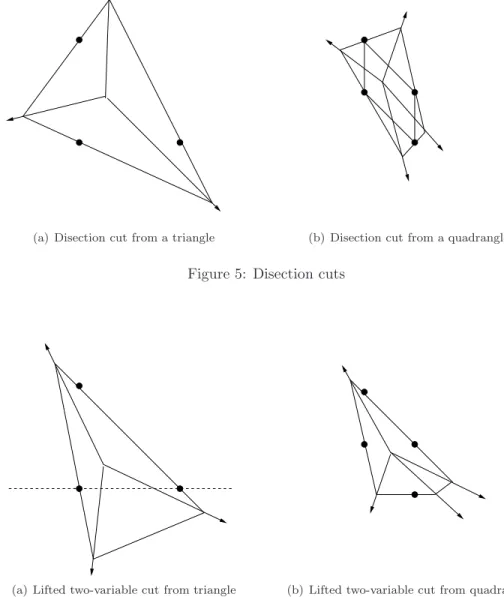
(i) Disection cuts (Fig. 5):
Every vertex of conv(Xα) belongs to a different facet of Lα.
(ii) Lifted two-variable cuts (Fig. 6):
Exactly one facet of Lα contains two vertices of conv(Xα). Observe that this implies that
there is a set S$ ⊂ S, |S$| = 2, such that!
j∈S"αjsj ≥ 1 is facet defining for conv(PI(S$)).
(iii) Split cuts:
Two facets of Lα each contain two vertices of conv(Xα).
(a) Disection cut from a triangle (b) Disection cut from a quadrangle
Figure 5: Disection cuts
(a) Lifted two-variable cut from triangle (b) Lifted two-variable cut from quadrangle
Figure 6: Lifted two-variable cuts
An example of a cut that is not a split cut was given in [4] (see Fig. 1). This cut is the only cut when conv(Xα) is the triangle of Fig. 4.(c), and, necessarily, Lα= conv(Xα) in this case. Hence,
all three rays that define this triangle are ray points. As mentioned in the introduction, the cut in [4] can be viewed as being on the boundary between disection cuts and lifted two-variable cuts. Indeed, by perturbing the three rays that define the triangle slightly, both a disection cut and a lifted two-variable cut can be obtained.
Since the cut presented in [4] is not a split cut, and this cut can be viewed as being a “boundary cut” between disection cuts and lifted two-variable cuts, a natural question is whether or not disection cuts and lifted two-variable cuts are split cuts. We finish this section by answering this question.
Lemma 10 Let !j∈Nαjsj ≥ 1 be a facet defining inequality for conv(PI) satisfying αj > 0 for
j ∈ N, and suppose none of the vertices of conv(Xα) are ray points. If !j∈Nαjsj ≥ 1 is a
disection cut or a lifted two-variable cut, then !j∈Nαjsj≥ 1 is not a split cut.
Proof: Observe that, if !j∈Nαjsj ≥ 1 is a split cut, then there exists (π, π0) ∈ Z2× Z such
that Lα is contained in the split set Sπ := {x ∈ R2: π0 ≤ π1x1+ π2x2 ≤ π0+ 1}. Furthermore,
all points x ∈ Xα and all vertices of Lα must be either on the line πTx = π0, or on the line
πTx = π
0+ 1. However, this implies that there must be two facets of Lα that do not contain any
integer points.
Example 3: Consider the set PI = {(x, s) ∈ Z2× R5+: x = f + ' 5 1 ( s1+ ' 5 13 ( s2+ ' −4 3 ( s3+ ' −2 −5 ( s4+ ' 0 −1 ( s5}, where f = ' 1 3 1 2 (
. We computed all the facets of conv(PI) for this example. In Table 1, we report
how many of the 25 facets belong to each of the categories defined above.
Disection Disection Lifted 2-var Lifted 2-var split
(triangle) (quadrangle) (triangle) (quadrangle) cut
# facets 3 3 1 14 4
percentage 12 12 4 56 16
Table 1: A categorization of the facets for an example
5
An algorithm to compute the vertices of conv(P
I)
In sections 3 and 4 we described the structure of the facets of conv(PI). In particular, we
demon-strated that every facet of conv(PI) can be obtained from a choice of at most four vertices of
conv(PI). Therefore, to compute the facets of conv(PI), a method for generating the vertices of
conv(PI) is needed, and this is the topic of this section.
It is well known that the facets of any mixed integer set can be computed from its polar. The polar of conv(PI) can be represented as a polyhedron by including one inequality for each extreme
point and each extreme ray of conv(PI). In our case, every extreme point (xv, sv) of conv(PI)
can be represented by two rays rjv and rkv, i.e., xv = s
jvr
jv + s
kvr
kv, where s
jv, skv ≥ 0 (Lemma
2.(iii)). Therefore, the polar of conv(PI) is the set of u ∈ Rn that satisfy
svjvujv + s
v
kvukv ≥ 1, for all vertices (x
v, sv) of conv(P I),
uj ≥ 0, for all j ∈ N,
where non-negativity follows from the extreme rays of conv(PI). To set up and optimize over
such a linear system, the vertices of conv(PI) must be computed. In this section, we present a
an overall algorithm that is based on optimizing over the polar of conv(PI) runs in polynomial
time.
Consider two arbitrary rays ri1 and ri2, where i
1, i2∈ N. We now show how to compute all
vertices of conv(PI) that can be obtained from ri1 and ri2. For simplicity assume i1 = 1, i2 = 2,
and let
PI(f, R) = {x ∈ Z2: x = f + r1s1+ r2s2, s1, s2≥ 0}, (24)
be the integer set generated from r1 and r2, where R := cone({r1, r2
}).
Observe that (24) can be reformulated by using a unimodular transformation. A unimodular transformation maps integer vertices to integer vertices and therefore preserves integrality. Observation 1 Let T ∈ Q2×2 be a unimodular matrix, and let {xv}
v∈V denote the vertices of
conv(PI(f, R)). Define ¯f := T f , ¯R := cone({T r1, T r2}) and ¯xv := T xv for v ∈ V . Then
conv(PI(f, R)) = conv({xv}v∈V) + R,
and
conv(PI( ¯f , ¯R)) = conv({¯xv}v∈V) + ¯R.
To simplify the exposition, we use a unimodular transformation to represent the problem in a standard form. This is achieved with a variant of the Hermite normal form (see [9]).
Observation 2 Let C ∈ Z2×2 be nonsingular. There exists a unimodular matrix T ∈ Q2×2 such
that (i) T C = ' 1 p 0 0 q0 ( , where q0≥ p0≥ 0.
(ii) The size of all entries in T C is polynomially bounded by the encoding length of C.
From Observations 1 and 2 it follows that we can assume r1 =
' 1 0 ( and r2 = ' p0 q0 ( . We now describe how to successively construct the vertices of conv(PI(f, R)). The algorithm
constructs a new vertex in every iteration, where the first vertex is trivially obtained as follows.
Lemma 11 The point w1 := (.f
1/, .f2/)T is a vertex of conv(PI(f, R)). Furthermore, the
in-equality x2≥ .f2/ is facet defining for conv(PI(f, R)).
Proof: This follows directly from the fact that R = cone({(1, 0)T, (p
0, q0)T)}, where p, q ≥ 0.
The remaining vertices of conv(PI(f, R)) are constructed in a particular order, which we now
discuss. If there exists a vertex w2 of conv(P
I(f, R)) with the same first coordinate as w1, then
we consider w2 as the “next” vertex of conv(P
I(f, R)). Observe that there can only be one such
vertex, and that this vertex, if it exists, can be constructed by simple rounding. In the following, we therefore assume for simplicity that no such vertex exists.
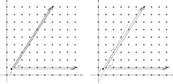
Now consider the set R2 := w1+ R with vertex w1 and extreme rays r1 and r2 (see Fig.
7.(a)). Observe that w1 is the only vertex of conv(P
I(f, R)) contained in R2. Therefore all the
remaining vertices of conv(PI(f, R)) are contained in the set (f + R) \ R2 (the hatched area of
Fig. 7.(a)). Furthermore, observe that the slope of the line between w1 and any remaining vertex
w of conv(PI(f, R)) is larger than the slope pq00 of r2 (see Fig. 7.(b)). The “next” vertex w2
is then defined to be the vertex w of conv(PI(f, R)) for which this slope is as large as possible.
Similarily, by induction, for any t ∈ {2, 3, . . . , r}, w(t−1)is the only vertex of conv(P
I(f, R)) in the
set Rt := w(t−1)+ R, and the “next” vertex wt is defined to be the vertex w of conv(PI(f, R)),
among the vertices that have not been chosen so far, for which the slope of the line between w(t−1)
f w1
(a) Initial vertex w1 and the set R 2 f w w 1 2
(b) The vertex w2and the corresponding facet Figure 7: Construction the vertex w2
We now introduce the following notation. For any k ∈ {2, 3, . . . , r}, let (pk, qk)T := wk−w(k−1).
Then the slope of the line between w(k−1) and wk is given byqk
pk, and by the choice of the ordering
w1, w2, . . . , wr of the vertices of conv(P
I(f, R)), we have that the slopes are ordered in decreasing
order q2 p2 > q3 p3 > . . . > qr pr .
Also note that all slopes are upper approximations to the slope q0
p0 of r
2, i.e., qk
pk >
q0
p0 for
all k = 2, 3, . . . , r, and that the approximation becomes better as k increases. The next lemma demonstrates that vertex wk can be obtained from the previous vertices w1, w2, . . . , w(k−1) by
solving an optimization problem.
Lemma 12 Let 2 ≤ k ≤ r. The pair (pk, qk) is an optimal solution to the optimization problem:
max q p s.t. q p≥ q0 p0 (25) w(k−1)+ ' p q ( ∈ f + R p, q∈ Z+.
Furthermore, there exists an optimal solution (ph, qh) to (25) and an integer δk
∈ Z+ such that
(pk, qk) = δk(ph, qh), and the set {(p, q) ∈ Z2 : (p, q) = δ(ph, qh), δ ∈ Z+ and 1 ≤ δ ≤ δk}
describes all optimal solutions to (25).
We now relate problem (25) to the directed simultaneous diophantine approximation problem. The directed simultaneous diophantine approximation problem D(qˆ
ˆ
the best upper approximation q
p of a rational number ˆ q ˆ
p under the constraint that p ≤ N
min q p s.t. q p≥ ˆq ˆp, (26) p≤ N, p, q∈ Z+.
The following theorem gives the relationship between the directed simultaneous diophantine approximation problem and problem (25).
Theorem 3 Assuming conv(PI(f, R)) does not have a vertex with the same first coordinate as w1,
the problem (25) has the same set of optimal solutions as the directed simultaneous diophantine approximation problem D(q0
p0, N ) with N = pk.
Proof: Consider the optimal solution (pk, qk) to (25). Also consider an optimal solution (¯p, ¯q) to
D(q0
p0, pk). We will prove that
qk
pk =
¯ q ¯
p. Note that this implies that every optimal solution (p∗, q∗)
to (25) must be optimal for D(q0
p0, pk) (since (p
∗, q∗) is feasible for D(q0
p0, pk) and attains the same
objective value as (¯p, ¯q)). Conversely every optimal solution (p$, q$) to D(q0
p0, pk) satisfies q" p" = qk pk, and since p$ ≤ p k, (p$, q$) is feasible for (25). We now prove qk pk = ¯ q ¯
p. Suppose, for a contradiction, that ¯ q ¯ p < qk pk. Clearly we have pk− ¯p ≥ 0,
since (¯p, ¯q) is feasible for (26), and we also have qk− ¯q ≥ 0, since qp¯¯< qpkk. We first argue that
w(k−1)+ ' pk− ¯p qk− ¯q ( ∈ f + R. (27)
Suppose (27) is not satisfied, i.e., we have the situation in Fig. 8. Observe that the slope of the line between the points w(k−1) and w(k−1)+ (¯p, ¯q) is identical to the slope of the line between
w(k−1)+ (p
k− ¯p, qk− ¯q) and w(k−1)+ (pk, qk), and that this slope is given by pq¯¯. Hence, if (27)
is not satisfied, then we have ¯q ¯ p <
q0
p0. However, this contradicts the fact that (¯p, ¯q) is feasible for
D(q0
p0, pk). Hence (27) is satisfied
Next suppose ¯p = pk. If also ¯q = qk, we are done, and if qk> ¯q, (27) implies that the vertical line
through w(k−1) contains integer points different from w(k−1) that are contained f + R. However,
this contradicts the assumption that conv(PI(f, R)) does not have a vertex with the same first
coordinate as w1.
Finally suppose pk > ¯p and qk > ¯q. Since pq¯¯<pqkk, we have
qk− ¯q
pk− ¯p
> qk pk
. (28)
Indeed (28) can be written as
pkqk− pk¯q > pkqk− qk¯p. (29)
It now follows from (28) and (27) that (pk− ¯p, qk− ¯q) is a feasible solution to (25) with a better
objective value than (pk, qk), which is a contradiction.
The optimal solutions of the directed simultaneous diophantine approximation problem D(q0
p0, N )
can be characterized from a minimal Hilbert basis of the cone R$= cone
'' 0 1 ( , ' p0 q0 (( , where a Hilbert basis of a rational polyhedral cone is defined as follows.
w
(k−1)w
(k−1)+
'
pk
qk
(
w
(k−1)+
'
¯
p
¯
q
(
w
(k−1)+
'
pk
− ¯p
qk
− ¯q
(
Figure 8: Existence of (¯p, ¯q)Definition 2 Let C ⊆ Rnbe a rational polyhedral cone. A finite set H(C) = {h1, . . . , ht
} ⊂ C∩Zn
is called a Hilbert basis of C if every z ∈ C ∩ Zn has a representation of the form
z =
t
"
i=1
λihi,
where λi ∈ Z+. Furthermore, if C is pointed, there exists a unique Hilbert basis H∗(C) of C of
minimum cardinality.
The following result is due to Henk and Weismantel [6].
Theorem 4 Let ˆp, ˆq ∈ Z+. For every N ∈ Z+, there exists an optimal solution to the
prob-lem D(qˆ ˆ
p, N ) defined by (26) which is a member of the Hilbert basis H∗(R$) of the cone R$ =
cone'' 01 (, ' ˆp
ˆq ((
. Conversely, for every member h of the Hilbert basis H∗(C) of R$, there
exists N ∈ Z+ such that h is an optimal solution of D(pˆqˆ, N ).
An algorithm to construct the vertices of conv(PI(f, R)) now follows directly from Theorem
3 and Theorem 4. We start from the vertex w1 = (.f
1/, .f2/). To construct the next vertex,
we consider the Hilbert basis elements of H∗(R$), where R$ = cone
'' 0 1 ( , ' p0 q0 (( . We sort the elements of H∗(R$) in terms of decreasing slopes. The first element h ∈ H∗(R$) for which
w1+ h ∈ f + R leads to the next vertex. Notice that, if there is a vertex of conv(P
I(f, R)) with
the same first coordinate as w1, then this vertex can be found using the element (0, 1) of H∗(R$),
which is always contained in H∗(R$). Also note that a similar approach has been used recently
by Agra and Constantino [1] to determine a complete description for multidimensional knapsack problems in two variables. The cones analyzed in [1], however, slightly differ from the family of cones studied here.
The algorithm above, however, does not run in polynomial time. It is well known that a Hilbert basis of a two-dimensional cone can be of exponential size. An algorithm, which is based on checking every element of H∗(R$), can therefore have exponential running time. Fortunately, we
can overcome this difficulty by exploiting the special structure of Hilbert bases of two-dimensional cones. A minimal Hilbert basis of a two-dimensional cone can be described by a polynomial number of vertices and edges (see [8]). The following theorem gives the structure of a minimal Hilbert basis of a two-dimensional cone in terms of vertices and edges.
Theorem 5 Let C = cone(r1, r2) ⊆ R2 be a rational polyhedral cone of dimension two. There
exists a polynomial number of vectors e1, . . . , es∈ Z2, called the edges, and numbers k1, . . . , ks∈
Z+ such that, if we denote the partial sums σ1i= !ij=1kjej,
H∗(R) = {r1,r1+ e1, . . . , r1+ k1e1= r1+ σ11, r1+ σ 11+ e2, . . . , r1+ σ11+ k2e2= r1+ σ12, ... r1+ σ 1(s−1)+ es, . . . , r1+ σ1s= r2 }.
We can now modify the initial algorithm as follows. Instead of checking every element of H∗(R$)
in turn, we sequentially check every edge of H∗(R$). This can be done in polynomial time using
binary search. To do this, consider the inverse of the matrix' 1 p0 q ( given by ' 1 −
p q 0 1 q ( . To check whether the elements e0+ je of the Hilbert basis H∗(R$) of R$ leads to a new vertex of
conv(PI(f, R)) from a previous vertex w(k−1) of conv(PI(f, R)), where j ∈ Z+and e, e0∈ Z2+ are
edges of H∗(R$), one needs to check the following condition
' 1 −p q 0 1 q ( (w(k−1)+ e 0+ je − f) ≥ ' 0 0 ( . (30)
The second inequality of (30) is trivially satisfied since w(k−1)
2 > f2. Hence the first inequality of
(30) determines whether an element of the Hilbert basis H∗(R$) along the edge e
0+ je provides
a new vertex of conv(PI(f, R)).
Example 4 Consider the cone
R = cone '' 1 0 ( , ' 237 1033 (( ,
and f = (2/3, 5/7). The edges of the Hilbert basis H∗(R$) = H∗(cone((0, 1), (1033, 237))) are given
by
(0, 1), (1, 4), (3, 13), (14, 61), (53, 231), (145, 632),
with k1= 1, k2= 2, k3= 3, k4= 2, k5= k6= 1. The algorithm takes the following steps.
Step 0 Construct the initial vertex w1= (.f
1/, .f2/) = (1, 1).
Step 1 Check the edge e1= (0, 1).
Find j such that (1, 1 + j) ∈ f + R. We obtain j ≤ 1.1, i.e., w2= (1, 2).
Step 2 Check the edge e2= (1, 4), i.e., Hilbert basis elements (j, 1 + 4j).
Find minimal j such that (1, 2) + (j, 1 + 4j) ∈ f + R.
We obtain j ≥ 2.4, i.e., we do not find a new vertex because j must be smaller than k2= 2.
Step 3 Check the edge e3= (3, 13), i.e., Hilbert basis elements (2 + 3j, 9 + 13j).
Find minimal j such that (1, 2) + (2 + 3j, 9 + 13j) ∈ f + R.
Step 4 Check the edge e4= (14, 61), i.e., Hilbert basis elements (11 + 14j, 48 + 61j).
Find minimal j such that (9, 37) + (11 + 14j, 48 + 61j) ∈ f + R. We obtain j ≥ 0.88. Hence j = 1, and w4= (34, 146).
Step 5 Check the edge e5= (53, 231), i.e., Hilbert basis elements (39 + 53j, 170 + 231j).
Find minimal j such that (34, 146) + (39 + 53j, 170 + 231j) ∈ f + R. We obtain j ≥ 1.19. Hence no new vertex is found.
Step 6 Edge e6= (145, 632) provides (237, 1033) as only Hilbert basis element. This is the extreme
ray of the translated cone.
The separation problem The method presented in this section can be used to compute all vertices of conv(PI) in polynomial time. For this, every pair of rays (O(n2)) must be considered,
and the vertices that can be obtained from this pair must be computed. Each subproblem provides a polynomial number of such vertices. To solve the separation problem, one can set up the polar of conv(PI) from the vertices of conv(PI). The polar includes an inequality for every vertex that
is not a ray point, and a nonnegativity constraints for every extreme ray.
References
[1] Agostinho Agra and Miguel Constantino. On the multiple integer knapsack polyhedra. 2005. [2] E. Balas. Intersection cuts - a new type of cutting planes for integer programming. Operations
Research, 19:19–39, 1971.
[3] E. Balas, S. Ceria, and G. Cornu´ejols. A lift-and-project cutting plane algorithm for mixed 0/1 programs. Mathematical Programming, 58:295–324, 1993.
[4] W.J. Cook, R. Kannan, and A. Schrijver. Chv´atal closures for mixed integer programming problems. Mathematical Programming, 47:155–174, 1990.
[5] R.E. Gomory. An algorithm for the mixed integer problem. Technical Report RM-2597, The Rand Corporation, 1960a.
[6] Martin Henk and Robert Weismantel. Diophantine approximations and integer points of cones. Combinatorica, 22(3):401–408, 2002.
[7] G.L. Nemhauser and L.A. Wolsey. Integer and combinatorial optimization. Wiley, 1988. [8] T. Oda. Convex bodies and algebraic geometry. Springer, New-York, 1985.
![Figure 1: The Instance in [4]](https://thumb-eu.123doks.com/thumbv2/123doknet/6545202.176405/3.918.237.652.74.495/figure-the-instance-in.webp)