*
S Supporting InformationABSTRACT: Over the last few decades, researchers have developed a number of empirical and theoretical models for the
correlation and prediction of the thermophysical properties of pure fluids and mixtures treated as pseudo-pure fluids. In this paper, a survey of all the state-of-the-art formulations of thermophysical properties is presented. The most-accurate thermodynamic properties are obtained from multiparameter Helmholtz-energy-explicit-type formulations. For the transport properties, a wider range of methods has been employed, including the extended corresponding states method. All of the thermophysical property correlations described here have been implemented into CoolProp, an open-source thermophysical property library. This library is written in C++, with wrappers available for the majority of programming languages and platforms of technical interest. As of publication, 110 pure and pseudo-purefluids are included in the library, as well as properties of 40 incompressible fluids and humid air. The source code for the CoolProp library is included as an electronic annex.
■
INTRODUCTIONA number of thermophysical property libraries exist that implement the highest-accuracy formulations for the thermo-physical properties offluids. The most widely used library is REFPROP,1a product of the United States National Institutes of Standards and Technology (NIST). In addition, there are a number of other thermophysical property libraries, each with varying capabilities and goals. These thermophysical property libraries are summarized in Table 1.
In addition, there are a few open-source thermophysical property libraries. Unfortunately, the state-of-the-art in open-source thermophysical property libraries is not very mature, apart from the CoolProp library presented here. The primary benefit of developing an open-source thermophysical library is that it facilitates easy collaboration because the source code can be read, modified, and improved by anyone in the world.
Furthermore, by developing a free, open-source, thermophys-ical property library, researchers all over the world can get access to state-of-the-art formulations for the thermophysical properties of fluids. Access to these high-accuracy properties will improve the quality of the research carried out in a wide range of technicalfields.
The major limitation of CoolProp, and most of the other libraries as well, is that they can not handle mixtures offluids. The treatment of mixtures offluids introduces a great amount of complexity and numerical challenges compared with the evaluation of the thermodynamic properties of purefluids. A description of the methods required for mixtures can be found in the literature.2−6
The state-of-the-art in thermodynamic property modeling is quite mature. Reference-quality equations of state, which can reproduce all experimental measurements within their exper-imental uncertainties, have been fit for a few pure fluids of technical interest. Methodologies have been proposed, such as thefixed form equation of state developed by Span and Wagner for polar7and nonpolar8fluids to more readily fit equations of state for other fluids for which less experimental data are available. Span et al.9provide a review of the state of art in the high-accuracy equations of state as of the year 2001.
Since the review of Span et al.9was published, high-accuracy equations of state have been published in the literature for sulfur hexafluoride,10 para-, ortho-, and normal hydrogen,11 propane,12 ethane,13 n-butane, and isobutane,14 penta fluoro-ethane (R125),15 ethanol16 and nitrogen.17 Additional pure fluid equations of state for cyclopentane,18
helium,19 propylene,20 refrigerant R227ea,21 refrigerant R365mfc,21 and
Received: October 10, 2013
Revised: January 2, 2014
Accepted: January 13, 2014
Published: January 13, 2014
Table 1. Software Packages Implementing High-Accuracy Equations of State for Pure and Pseudo-pure Fluids
library name reference fluids
open-source mixtures notes REFPROP 9.1 1 127 no yes wrappers
available for numerous languages CoolProp 4.0 23 110 yes no wrappers
available for numerous languages EES 24 88 no limited FLUIDCAL 25 70 no no Zittau 26 34 no no FPROPS 27 36 yes no
HelmholtzMedia 28 9 yes no only for use with Modelica
Solkatherm 3622 have been constructed by other researchers that have not yet been published as of publication.
From the standpoint of transport property modeling, the state-of-the-art is less mature. Partly, this is due to the fact that, in order to develop a high-accuracy transport property correlation, a high-accuracy formulation for the thermodynamic properties is required in order to evaluate the density for given temperature and pressure. For that reason, there tends to be at least a few years lag between the publication of the equation of state and the transport property correlations. In addition, there is a general shortage of experimental data of transport properties.
In recent years, a number of high-accuracy correlations for transport properties have been developed, and as of publication, 36 fluids have fluid-specific correlations for their transport properties. These fluids are summarized in a table in the Supporting Information.
■
THERMODYNAMIC PROPERTIESThe thermodynamic properties of all the fluids that are implemented in CoolProp are based on Helmholtz-energy-explicit equations of state. This formulation is currently employed for all the high-accuracy equations of state that are available in the literature. Span29provides further information on this formulation. Furthermore, equations of state based on the Bender30 or modified Benedict−Webb−Rubin (mBWR) forms can be converted to Helmholtz-energy-explicit forms using the methods presented in Span.29
In the Helmholtz-energy-explicit formulation, the total nondimensionalized Helmholtz energy α can be given as the sum of two contributions: the residual (αr) and ideal-gas (α0)
parts. Thus, the nondimensionalized Helmholtz energy can be given by
α= α0+αr (1)
The elegance of this formulation is that all other thermodynamic properties can be obtained through analytic derivatives of the termsα0 andαr. For instance, the pressure can be obtained from
ρ δ α δ = = + ∂ ∂ τ ⎛ ⎝ ⎜ ⎞⎠⎟ Z p RT 1 r (2)
where Z is the compressibility factor, p is the pressure in kPa,ρ is the density in kg·m−3, R is the mass specific gas constant in kJ·kg−1·K−1, T is the temperature in Kelvin, the reduced density δ is given by δ = ρ/ρred, and the reciprocal reduced temperature
is given byτ = Tred/T.
The reducing density ρred is generally the critical densityρc
and the reducing temperature Tred is generally the critical temperature Tc. For the pseudo-pure fluids (Air, R404A,
R410A, R407C, R507A, and SES36), selected siloxanes (MM, MD4M, D4, and D5), refrigerant R134a, and methanol, the
reducing parametersρredand Tredare determined as part of the fitting process.
The other fundamental thermodynamic properties can be obtained directly using the fundamental equation of state. The enthalpy is obtained from
τ α τ α τ δ α δ = ∂ ∂ + ∂ ∂ + ∂ ∂ + δ δ τ ⎡ ⎣ ⎢ ⎢ ⎛ ⎝ ⎜ ⎞ ⎠ ⎟ ⎛⎝⎜ ⎞⎠⎟ ⎤ ⎦ ⎥ ⎥ ⎛ ⎝ ⎜ ⎞⎠⎟ h RT 1 0 r r (3)
where h is the enthalpy in kJ·kg−1, and the entropy is obtained from τ α τ α τ α α = ∂ ∂ + ∂ ∂ − − δ δ ⎡ ⎣ ⎢ ⎢ ⎛ ⎝ ⎜ ⎞ ⎠ ⎟ ⎛⎝⎜ ⎞ ⎠ ⎟ ⎤ ⎦ ⎥ ⎥ s R 0 r 0 r (4)
where s is the entropy in kJ·kg−1·K−1.
Additionally, other thermodynamic parameters (speed of sound, specific heats, derivatives, etc.) can be obtained analytically. Lemmon et al.5 and Span29 provide thorough coverage of these derivatives and thermodynamic properties. Furthermore, other combinations of partial derivatives, as well as analytic derivatives along the saturation curves and in the two-phase region can be found in the work of Thorade and Sadat.31
The Helmholtz-energy-explicit equations of state use temperature and density as the independent variables. If other state variables are given, it is necessary to employ numerical solvers to obtain temperature and density given the other set of inputs. Span32provides a description of how to handle the input state variables of temperature/pressure, pressure/density, pressure/enthalpy, and pressure/entropy. Additionally, a solver for enthalpy/entropy inputs has been implemented in CoolProp.
■
HELMHOLTZ ENERGY COMPONENTSResidual Component. In general, the form of the residual Helmholtz energy is fluid dependent and is obtained by an optimization routine that selects terms from a large library of candidate terms. This process is described in some depth in the literature.5,15,29,33 For the residual Helmholtz energy term, there are generally six families of terms that have been employed throughout the equations of state. The residual Helmholtz energy is given by a summation
∑
α = α k r k r (5)where each termαkris differentiable analytically with respect to
δ and τ.
The types of terms that have been used in the literature in equations of state are
Power family33
∑
αk = nδ τ i i d t r i i (6)Exponential in reduced density32
∑
αk = nδ τ exp(−γδ ) i i d t i c r i i i (7)Exponential in reduced density and reciprocal reduced temperature34
∑
αk = nδ exp(α τ−γδ ) i i d i i c r i i (8) Gaussian family33∑
αk = nδ τ exp(−η δ( −ε) − β τ( −γ) ) i i d t i i i i r i i 2 2 (9)Exponentials inδ and τ family15
∑
αk = nδ τ exp(−δ )exp(−τ ) i i d t c m r i i i i (10)Nonanalytic term33
∑
αk = nΔδψ i i b r i (11) where θ δ Δ = 2+B [(i − 1) ]2 ai (12) θ= (1−τ)+Ai[(δ−1) ]2 1/(2 )βi (13) ψ=exp(−Ci(δ− 1)2 −Di(τ− 1) )2 (14)Analytic partial derivatives of each family with respect to τ andδ up to the second order derivatives can be found in the referenced paper for each family. Furthermore, the values for the coefficients ni, ti, di, etc. are presented in each equation of state. All the permutations of third order partial derivatives have also been implemented in CoolProp. These higher order analytic derivatives are required in order to implement analytic derivatives for the Tabular Taylor Series Expansion (TTSE) method35or bicubic interpolation as described below.
Ideal Gas Component. Like the residual Helmholtz energy, the form of the ideal-gas part of the Helmholtz energy is also fluid dependent. The ideal-gas Helmholtz energy is obtained from the relationship
∫
∫
α ρ ρ = − + + − + − T T h RT s R T c T R T c T RT T 1 ln 1 ( )d ( ) d T T T T 0 0 0 0 0 0 0 p0 p 0 0 0 (15)and thus, the ideal-gas part of the Helmholtz energy can be obtained if the reference state parametersρ0, T0, h00, and s
0 0are
specified and the ideal-gas isobaric specific heat cp0(T)/R
relationship is known. The reference state parametersρ0, T0, h00,
and s00 are selected in order to yield the desired values for
enthalpy and entropy at the reference state. The integration in eq 15 must be carried out in order to use the ideal-gas contribution in the equation of state.
Over the years numerous forms for the ideal-gas specific heat have been implemented, including Plank−Einstein terms,33 Aly−Lee terms,36and polynomial terms.
Vapor−Liquid Equilibrium. In the vapor−liquid two-phase region, as well as along the saturation curves, it is necessary to evaluate the phase equilibrium between the saturated liquid and the saturated vapor.
For a purefluid at equilibrium, the temperatures, pressures and Gibbs free energy in each phase are the same. Thus, for a given saturation temperature Ts, the system of equations to be
solved is
ρ′ = ρ″
p T( ,s ) p T( ,s ) (16)
ρ′ = ρ″
g T( ,s ) g T( ,s ) (17)
where the unknowns are the saturated liquid densityρ′ and the saturated vapor densityρ″.
The method proposed by Akasaka37is employed, which is a two-dimensional Newton−Raphson solver for the nonlinear system of equations from eqs 16 and 17. For a given temperature Ts, this method yields the solutions for the
saturation pressure ps, the saturated liquid densityρ′ and the saturated vapor densityρ″. Figure 1 shows the saturation curves for all thefluids included in CoolProp in reduced coordinates. This solver begins with initial guess values for ρ′(T) and ρ″(T) provided by the ancillary equations. For fluids without published ancillary curves, ancillary curves for ρ′(T), ρ″(T), and p(T) have beenfit using routines provided in the CoolProp package. In general, the combination of highly accurate ancillary equations and the Newton−Raphson method yields proper convergence for temperatures where Tt < T < (Tc−0.01 K)
where Ttis the triple point temperature. When the Newton− Raphson method fails with the normal method, a relaxation parameter can be introduced to yield better convergence behavior in the near-critical region.
In the near vicinity of the critical point, the behavior of the saturation solvers becomes significantly less robust, even with good guess values for the saturation densities from the ancillary equations. As a result, it is necessary to employ other methods to extend the saturation curves all the way up to the critical temperature. The solvers presented above are used to get as close to the critical temperature as possible. Beyond that point, a spline curve is used for the saturation curve, where the value and derivative constraints can be obtained from the last point that the Newton−Raphson method succeeded at temperature Tend. The constraints on the spline for the saturated liquid density are ρ|T T=c =ρc (18) ρ ∂ ∂ ′ = = T 0 T Tc (19) ρ|T T= = ′ρ(Tend) end (20)
ρ ρ ∂ ∂ ′ = ∂ ∂ ′ = T T T ( ) T T end end (21)
where the right-hand side of each constraint is evaluated analytically from the equation of state. A similar spline is constructed for the saturated vapor density as a function of the temperature. This yields a smooth (C1continuous) transition from the EOS to the critical region spline. Furthermore, the critical spline is imposed to yield the correct value for the density at the critical point. For eachfluid, the value of Tendand
the saturation derivatives at Tendare precalculated and cached in order to maximize computational efficiency.
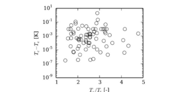
Figure 2 shows the range of the saturation curve that is treated using a spline curve as a function of the ratio of the
critical temperature to the triple point temperature. Forfluids with well constructed equations of state and good ancillary equations, the numerical VLE solver succeeds at temperatures within 1 × 10⁻⁹ K of the critical temperature, but for refrigerants R11 and R14, the saturation solvers fail at a distance greater than 0.1 K from the critical point.
It is a common need to obtain the saturation temperature for a given saturation pressure. The saturation pressure curves as a function of temperature are continuous from the triple point temperature to the critical point temperature. Somefluids have equations of state where the minimum temperature is above the triple point temperature. Therefore, it is straightforward to obtain the saturation temperature for the given saturation pressure.
There are several means of implementing this solution procedure. The most robust is the use of Brent’s method,38 which is a bounded one-dimensional solver with quadratic updates and guaranteed convergence. Brent’s method38is used to drive the residuum
= −
T p T p
RES( )s s( )s target (22)
to zero. The saturation temperature Ts is the independent variable, which is known to lie within the closed range between the triple point temperature and the critical point temperature. The solution is found when the saturation pressure ps(Ts)
(evaluated from the vapor−liquid equilibrium solver routine) is equal to the target pressure ptarget.
In the case of pseudo-pure fluids (Air, refrigerant R404A, refrigerant R410A, etc.), it is not possible to determine the vapor−liquid equilibrium with the use of the phase equilibria from eqs 16 and 17. For these mixtures, at equilibrium, the mole fractions of each component are not the same in the vapor and liquid phases and the pseudo-purefluid equation of
state can only calculate properties for the pseudo-pure fluid composition. The saturated liquid and vapor ancillary pressure equations are thus no longer optional but required to calculate the saturation pressures. The pressures calculated from the ancillary equations are then used to evaluate the saturation densities using the equation of state.
■
INTERPOLATION METHODSWhen using equations of state in engineering applications, computational efficiency is of the utmost importance. In order to improve the speed of evaluation of the equation of state, interpolation methods can be used. While a comparison of interpolation methods is beyond the scope of this work, two interpolation methods that have been found to yield excellent behavior are the Tabular Taylor Series Expansion (TTSE) method and the bicubic interpolation method. These two methods share the requirement that values of state variables are tabulated on a regularly (either linearly or logarithmically) spaced grid, as well as derivatives of the state variable with respect to the two independent variables.
Using the TTSE method, with pressure and enthalpy as independent variables, the temperature can be obtained from the expansion = + Δ ∂ ∂ + Δ ∂ ∂ + Δ ∂ ∂ + Δ ∂ ∂ + Δ Δ ∂ ∂ ∂ ⎜ ⎟ ⎛ ⎝ ⎞⎠ ⎛ ⎝ ⎜ ⎞ ⎠ ⎟ ⎛ ⎝ ⎜ ⎞ ⎠ ⎟ ⎛ ⎝ ⎜ ⎞ ⎠ ⎟ ⎛ ⎝ ⎜ ⎞ ⎠ ⎟ T T h T h p T p h T h p T p h p T p h 2 2 i j p h p h , 2 2 2 2 2 2 2 (23)
where the derivatives are evaluated at the point i,j, and the differences are given by Δp = p − pj and Δh = h − hi. The
nearest state point can be found directly due to the regular spacing of the grid of points. Pressure and enthalpy are very common state variable inputs in the simulation of thermal engineering systems.
For an improved representation of the p−v−T surface, bicubic interpolation can be used. In the bicubic interpolation method, the state variable and its derivatives are known at each grid point. This information is used to generate a bicubic representation for the property in the cell, which could be expressed as
∑ ∑
= = = T x y( , ) a x y i j ij i j 0 3 0 3 (24)where aijare constants based on the cell boundary values and x
and y are normalized values for the enthalpy and pressure, for instance. The constants aijin each cell are cached for additional
computational speed.
As an example of the increase in computational speed possible through the use of these interpolation methods, the density is calculated as a function of the pressure and enthalpy for subcooled water. The IAPWS 1995 formulation for the equation of state of ordinary water33 is one of the most involved equations of state in the literature. For subcooled water at a pressure of 10 MPa and an enthalpy of 475 kJ·kg−1 (where the reference enthalpy is 0.611872 J·kg−1 for the saturated liquid at the triple point), both the TTSE method and the bicubic interpolation method are more than 120 times faster than the evaluation of the density from the equation of state (it takes approximately 1μs to evaluate density using the TTSE or bicubic interpolation methods). Thus, using one of
Figure 2.Range of critical spline versus the ratio of critical to triple point temperatures forfluids with Tc− Tend> 1× 10⁻⁷K.
these interpolation methods can yield a reduction in computa-tional time of greater than 98%.
Practical implementation of these methods involves building tables with thefluid properties and their derivatives at each grid point. This task is only performed at thefirst property call and takes only a few seconds. The tables are then cached for further use.
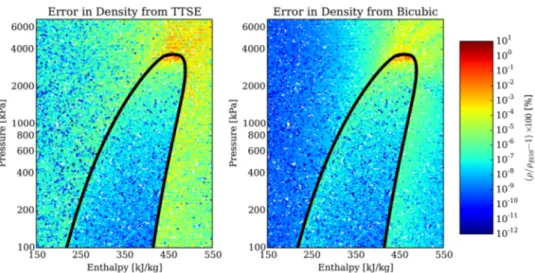
As another example of the accuracy of these interpolation methods, the density of refrigerant R245fa is evaluated at 40000 data points covering the entirefluid surface. Figure 3 shows the results of this analysis. These data show that the accuracy of the bicubic interpolation method is generally several orders of magnitude better than that of the TTSE method, though both yield acceptable accuracy for most technical needs.
■
TRANSPORT PROPERTIESFor the transport properties (here viscosity, thermal con-ductivity, and surface tension), the state-of-the-art is less mature. A wider range of methodologies have been employed to correlate and/or predict these properties. For a number of fluids, high-accuracy fluid-specific correlations have been developed based on wide-ranging experimental data, but for others, little or no experimental data are available and predictive or empirical methods must be employed.
■
PURE FLUID CORRELATIONSViscosity. Correlation of the viscosity of pure fluids is typically divided into two contributions: one part provides the temperature-dependent viscosity in the zero-density limit (dilute-gas), and the second part considers the temperature-and density-dependent residual viscosity, as in
η =η(0)( )τ +η( )r( , )τ δ (25)
For a very restricted subset of fluids, there is sufficient information about viscosity in the critical region to consider the critical enhancement of the viscosity. In general, the critical enhancement of viscosity is not considered. Of all the purefluid viscosity correlations developed, the only ones with a critical enhancement term for the viscosity are ordinary water39 and carbon dioxide.40
It is possible to theoretically treat the zero-density viscosity using Chapman−Enskog theory, which yields the dilute gas viscosity of η σ = × Ω η − MT (26.692 10 ) (0) 3 2 (2,2) (26)
whereη(0)is the viscosity in the limit of zero density inμPa·s, M is the molar mass in kg·kmol−1, T is the temperature in Kelvin,σηis the size parameter of the Lennard-Jones model in
nm, and Ω(2,2) is the empirical collision integral given by the
form from Neufeld41
Ω = * + − * + − * − T T T 1.16145( ) 0.52487 exp( 0.77320 ) 2.16178 exp( 2.43787 ) (2,2) 0.14874 (27)
where T* is the reduced temperature defined by T* = kT/εη and where the ratio εη/k of the pair potential energy to
Boltzmann’s constant is in Kelvin and is fluid dependent. For fluids that are well characterized by experimental data, it is possible to fit the term Ω(2,2) to experimental data. Also, for
fluids for which the terms σηandεη/k are unknown, they can be
estimated based on the method from Chung et al. in eqs 51 and 52.
The residual viscosity η(r) can be treated in a variety of
different ways. In older viscosity correlations, it was common practice to develop an empirical correlation forη(r)directly. In
the last 15 years, the preponderance of pure fluid viscosity correlations42−44 have been based on the division of the residual viscosity into a theoretically derived initial-density term from Rainwater−Friend theory45,46 and a higher-order correction term. Thus, the residual viscosity is given by
where Bηis the second viscosity virial coefficient in L·mol−1,ρ̅ is the molar density of the fluid in mol·L−1, and Δηh is the
higher order correction term inμPa·s.
The second viscosity virial coefficient is given by
σ
= *
η η η
B 0.6022137 3B (29)
whereσηis the molecular size in nm, and T* = T/(εη/k) and with
Figure 3.Comparison of the accuracy of TTSE and bicubic interpolation methods for refrigerant R245fa (interpolation grid is 200× 200, enthalpy spaced linearly, pressure spaced logarithmically).
∑
* = * + * + * η = − − − B b T( ) b T( ) b T( ) i i i 0 6 0.25 7 2.5 8 5.5 (30)The coefficients biare from Vogel et al. 42
and are duplicated in Table 2 for completeness.
The higher-order term is often of a form similar to the free-volume term proposed by Batschinski47 and Hildebrand.48 A general form of the higher-order term is given by
∑ ∑
η δ δ δ δ δ δ δ Δ = + − − = = ⎡ ⎣ ⎢ ⎤ ⎦ ⎥ T e T f T T ( , ) ( ) ( ) i n j m ij i j h r 2 0 r 1 0 r 0 r (31)whereΔηhis inμPa·s, Tr= T/Tred, and the coefficients eijand f1 arefit for each fluid. Furthermore, the term δ0(Tr) is given by
the form
∑
δ = + = − T g g T ( ) (1 ) i i i 0 r 1 2 5 r ( 1)/2 (32)where the coefficients giare alsofit for the given fluid.
It should also be mentioned that the generalized friction theory model has been successfully applied to the prediction of the viscosity of somefluids, notably the n-alkanols,49hydrogen sulfide,50 and sulfur hexafluoride.51 Currently, the generalized friction theory method remains less used in the reference literature than the viscosity correlation method outlined here.
Thermal Conductivity. The correlations for thermal conductivity are decomposed into three terms, yielding the following form:
λ=λ(0)( )τ +λ( )r( , )τ δ +λ( )c( , )τ δ (33)
where each term is in mW·m−1·K−1.
Unlike viscosity (where the critical enhancement term is very small except in the immediate vicinity of the critical point), the critical enhancement term for thermal conductivityλ(c)is
non-negligible well away from the critical point.
The dilute gas term in the limit of zero-density λ(0) is
typically correlated with the temperature using a body of low-density thermal conductivity measurements, which usually results in a short polynomial form similar to
∑
λ = a T i i i (0) (34)The residual term is often given by a form similar to
∑
λ = + δ = B B T ( ) r i n i i i ( ) 1 1, 2, r (35)Finally the critical enhancement term needs to be considered. The most commonly used critical enhancement term used is the simplified critical enhancement term of Olchowy and Sengers:52 λ ρ πηζ = (10 ) c R kT Ω − Ω 6 ( ) c ( ) 12 p D 0 (36) π ζ ζ Ω = − + ⎡ ⎣ ⎢ ⎢ ⎛ ⎝ ⎜⎜ ⎞⎠⎟⎟ ⎤ ⎦ ⎥ ⎥ c c c q c c q 2 arctan( ) p v p d v p d (37) π ζ ζρ ρ Ω = − − + − ⎡ ⎣ ⎢ ⎢ ⎛ ⎝ ⎜⎜ ⎞⎠⎟⎟⎤ ⎦ ⎥ ⎥ q q 2 1 exp 1 ( ) ( / ) /3 0 d 1 d c 2 (38) ζ ζ ρ ρ ρ ρ ρ ρ = Γ ∂ ∂ − ∂ ∂ ν γ ν γ ⎛ ⎝ ⎜⎜ ⎞⎠⎟⎟ ⎡ ⎣ ⎢ ⎢ ⎤ ⎦ ⎥ ⎥ p T p T T T p ( , ) ( , ) T T 0 c c 2 / R R / (39)
whereλ(c)is in mW·m−1·K−1,ζ is in m, cpand cvare in kJ·kg−1·
K−1, p and pc are in kPa, ρ and ρc are in kg·m−3, η is the viscosity inμPa·s, and the remaining parameters are defined in Table 3. The factor 1012 is a unit conversion parameter that
yields a thermal conductivity in mW·m−1·K−1.
Surface Tension. Mulero et al.54
have recently refit correlations for the surface tension of nearly all thefluids in REFPROP 9.0.55These correlations are each of the form
∑
σ = ⎛ − ⎝ ⎜ ⎞ ⎠ ⎟ a T T 1 i i n c i (40)where σ is the surface tension in mN·m−1, Tc is the critical temperature in Kelvin, and ai and ni are correlation constants.
This formulation ensures that the surface tension goes to zero at the critical point. The mean absolute percentage difference of each of these correlations is less than 6%, and most are below 3%.
For fluids that are not included in the database of Mulero, the following general form from Miqueu et al.56is employed
σ = ⎛ + ω + − ⎝ ⎜ ⎞ ⎠ ⎟ kT N V (4.35 4.14 )t (1 0.19t 0.25 )t c A c 2/3 1.26 0.5 (41)
where σ is the surface tension in N·m−1, k is the Boltzmann constant (k = 1.3806488 × 10⁻²³ J·K−1), Tc is the critical temperature in Kelvin, NA is Avogadro’s number (NA =
Table 2. Coefficients for the Second Viscosity Virial Coefficient in Equation 30
b0 −19.572881 b1 219.73999 b2 −1015.3226 b3 2471.01251 b4 −3375.1717 b5 2491.6597 b6 −787.26086 b7 14.085455 b8 −0.34664158
Table 3. Coefficients for Use in the Simplified Olchowy-Sengers Critical Term in Equations 36 to 39
Universal Constants Boltzmann constant k 1.3806488× 10⁻²³J·K−1 universal amplitude RD 1.03 critical exponent ν 0.63 critical exponent γ 1.239 reference temp. TR 1.5Tc
Recommended Default Constants53
amplitude Γ 0.0496
amplitude ζ0 1.94× 10⁻¹⁰m effective cutoff qd 2× 10⁹m
conductivity over the wholefluid surface, and one method that has been used successfully is the method of extended corresponding states. In this method, the transport properties for the fluid of interest are obtained from the transport properties for a well-characterized reference fluid. The reference fluid selected should have high-accuracy transport property measurements as well as have a p−v−T surface that is similar in shape to thefluid of interest.
The analysis in this section follows the method proposed by Huber et al.,53 which has been implemented in REFPROP.1 The primary contribution of this section on the extended corresponding states is the presentation of a small set of example data that can be used to validate the implementation of the extended corresponding states method. No validation data for extended corresponding states has been published before. These example data are provided in Table 4 to allow for proper validation of the implementation of the extended correspond-ing states method.
In the analysis that follows in this section, the subscript ⊥ refers to the referencefluid, and ◊ refers to the fluid of interest. Molar specific quantities are given with an overbar, and mass-specific quantities do not have an overbar.
Conformal State. The conformal state is the thermody-namic state point for the referencefluid that is used to evaluate the reference-fluid contribution to the extended corresponding states method. This conformal state point is determined based on the equivalent substance reducing ratios f and h of
ρ ρ = = ̅ ̅ ◊ ⊥ ⊥ ◊ f T T h (42)
or alternatively expressed in terms of shape factorsθ and ϕ
θ ρ ρ ϕ = = ̅ ̅ ◊ ⊥ ⊥ ◊ f T T h c, c, c, c, (43)
The corresponding states method is most accurately applied to monatomic gases, and the shape factor can be thought of as a term that accounts for deviation from spherical molecular geometry. The shape factor can be approximated based on one of several empirical forms that have been proposed, such as those from Erickson and Ely60(for the referencefluid propane) of θ= 1+(ω◊−ω⊥)(a1+a2ln(T T◊/ c,◊)) (44) ϕ = ⊥ + ω −ω + ◊ ◊ ⊥ ◊ ◊ Z Z [1 ( )(a a ln(T T/ ))] c, c, 3 4 c, (45) with a1= 0.5202976, a2=−0.7498189, a3= 0.1435971, and a4 = −0.2821562 or by the more general solution (of a similar
form) from Estella−Uribe and Trusler,61
which provides higher fidelity predictions in the critical region.
For the highest accuracy and generality (shape factors independent of the referencefluid selected), it is preferable to use the“exact” shape factors, which are obtained through the use of the equations of state of the fluid of interest and the referencefluid.
The“exact” shape factors are defined based on the conformal state T⊥, ρ⊥ of the reference fluid. The conformal state is
defined by equating the compressibility factor and the residual component of the Helmholtz energy of the referencefluid and thefluid of interest,53,62,63
ρ = ρ ⊥ ⊥ ⊥ ◊ ◊ ◊ Z T( , ) Z T( , ) (46) and α⊥(T⊥,ρ⊥)=α◊(T◊,ρ◊) r r (47)
The right-hand side of each equation is known for thefluid of interest. Thus, it simply remains to obtain the conformal state point T⊥,ρ⊥from a simultaneous solution of the two equations. The most straightforward solver to be used is a conventional two-dimensional Newton nonlinear system of equations solver. The Newton method for the conformal state solver can be given by xk+1 = xk + v where xk is the vector ⟨τ⊥,k, δ⊥,k⟩ and where v is obtained by solving the system of equations Jv =−r
ψη[−] 1.0454 η◇(0)[μPa·s] 13.617 Fη[−] 1.60328 η⊥(r)(T⊥,ρ̅⊥ψη) [μPa·s] 77.61535 η [μPa·s] 138.056 η [μPa·s] (REFPROP 9.1) 138.056 Conductivity ψλ[−] 1.0583 fint[−] 0.0014 λ◇int[mW·m−1·K−1] 12.411 λ◇* [mW·m−1·K−1] 3.111 Fλ[−] 0.51802 λ⊥(r)(T⊥,ρ̅⊥ψλ) [mW·m−1·K−1] 70.24348 λ◇c [mW·m−1·K−1] 0.884 λ [mW·m−1·K−1] 52.794 λ [mW m−1·K−1] (REFPROP 9.1) 52.794 Correlations59 ψλ= 1.0898− 1.54229 × 10⁻²δ fint= 1.17690× 10⁻³+ 6.78397× 10⁻⁷T ψη= 1.04253 + 1.38528× 10⁻³δ
aNote: Both CoolProp and REFPROP implement the EOS for
propane from Lemmon et al.,12 which causes errors in viscosity prediction of propane of up to 2%.
and the Jacobian matrix for the solver can be given analytically by α τ ρ α δ δ α τ δ ρ δ α δ α δ = − ∂ ∂ ∂ ∂ − ∂ ∂ ∂ ∂ ∂ + ∂ ∂ ⊥ ⊥ ⊥ ⊥ ⊥ ⊥ ⊥ ⊥ ⊥ ⊥ ⊥ ⊥ ⊥ ⎡ ⎣ ⎢ ⎢ ⎢ ⎢ ⎢ ⎛ ⎝ ⎜ ⎞ ⎠ ⎟ ⎤ ⎦ ⎥ ⎥ ⎥ ⎥ ⎥ T T T T J 1 1 c c c c , 2 r , r , 2 2 r , 2 r 2 r (48)
where each of the partial derivatives are evaluated at the state point T⊥,ρ⊥. The residual vector r is given by
α ρ α ρ ρ ρ = − − ⊥ ⊥ ⊥ ◊ ◊ ◊ ⊥ ⊥ ⊥ ◊ ◊ ◊ ⎡ ⎣ ⎢ ⎢ ⎤ ⎦ ⎥ ⎥ T T Z T Z T r ( , ) ( , ) ( , ) ( , ) r r (49)
This solver generally yields good convergence behavior when started at the initial guess value defined by θ = 1 and ϕ = 1.
At very low densities, the conformal solver may fail, which can be avoided by only evaluating the conformal state for densities of thefluid of interest above 1.0 kg·m−3. Below this density, the conformal state is determined by assumingθ = 1 andϕ = 1. This treatment introduces a small discontinuity in the conformal state at the density of 1.0 kg·m−3, but in the dilute gas domain, both the viscosity and thermal conductivity are dominated by the dilute gas contribution.
Viscosity. In the extended corresponding states method, the viscosity is divided into two contributions, one for the dilute gas contribution in the limit of zero density, and another for the residual contribution. This division is analogous to the separation employed forfluid-specific viscosity correlations(see eq 25). Thus the viscosity can be given by
η◊= η◊(0)( )τ +ηECS( )r ( , )τ δ (50)
whereη◊is the viscosity of thefluid of interest in μPa·s, η◊(0)is the dilute-gas viscosity contribution of thefluid of interest in μPa·s, and ηECS(r) is the residual contribution from the extended
corresponding states method, inμPa·s.
The dilute gas contributionη◊(0)can be treated theoretically and is obtained from the eqs 26 and 27. If the Lennard-Jones parametersεη/k andσηare unknown for thefluid of interest, they can be obtained from the method from Chung et al.64
ση=0.809/( )ρc̅ 1/3 (51)
εη/k=Tc/1.2593 (52)
where ση is in nm, ρ̅c is in mol·L−1 and Tc and εη/k are in
Kelvin. Ifεη/k and σηare known for a referencefluid but not thefluid of interest, these values for the fluid of interest can be obtained from the method proposed in Huber et al.53of
εη ◊ = εη ⊥ ◊ ⊥ ⎛ ⎝ ⎜⎜ ⎞⎠⎟⎟ k k T T ( / ) ( / ) c, c, (53) σ σ ρ ρ = ̅ ̅ η◊ η⊥ ◊ ⊥ ⎛ ⎝ ⎜⎜ ⎞ ⎠ ⎟⎟ , , c, c, 1/3 (54)
which is simply the application of the method of Chung et al.64 to both the referencefluid and the fluid of interest. It should be emphasized that molar densities must be used in eq 54.
The Lennard-Jones parametersεη/k andσηfor a number of fluids can be found in the works of Chichester and Huber65
and Poling et al.66
The residual contribution to the viscosity is obtained using the residual viscosity of the referencefluid. To begin with, the conformal temperature T⊥and conformal molar densityρ̅⊥are
obtained using the methods presented in the conformal state section. For somefluids, there are sufficient experimental data in order tofit a simple polynomial correction in the reduced density of thefluid of interest of the form
∑
ψη= cδ◊
i i i
(55)
This correction term shifts the density of the referencefluid used in the viscosity correlation away from the conformal density. If no experimental information is available to obtainψη, ψηis assumed to be equal to 1.0. Huber et al.,53McLinden et
al.,62 and Klein et al.67 provide some of the only published values for these correction polynomials. Significant work has been carried out by the authors of REFPROP to develop correction polynomials, but the density correction polynomials in REFPROP are not in the public domain.
Thus, the extended corresponding states contribution to the viscosity is obtained from
η ( , )τ δ =Fη·η⊥ (T⊥,ρ ψ⊥̅ η) r r ECS ( ) ( ) (56) whereη⊥(r)(T
⊥,ρ̅⊥ψη) is the contribution of the residual viscosity
from the referencefluid evaluated at the temperature T⊥ and
the molar densityρ̅⊥ψη. The residual viscosity of the reference fluid includes all the density-dependent terms of the viscosity correlation, which, based on the formulation in the prior section, would be the contribution from eq 28. Fηis a factor
that arrives from the fact that the corresponding states theory states that the viscosity of twofluids at the same reduced state are equivalent.67Fηcan be given by
= η − ◊ ⊥ F f h M M 1/2 2/3 (57)
where h and f are the equivalent substance reducing ratios obtained from the conformal state solver, and M◊and M⊥are the molar masses of thefluid of interest and the reference fluid, respectively, each in kg·kmol−1.
Thermal Conductivity. A similar protocol is used to calculate the thermal conductivity using extended correspond-ing states. Again, the division of terms for thermal conductivity is similar to that offluid-specific correlations(see eq 33). The thermal conductivity is divided into four terms, as in
λ◊=λ◊int( )τ +λ◊*( )τ + λECS( )r ( , )τ δ +λ◊(c)( , )τ δ (58)
whereλ◊int is the internal thermal conductivity contribution of
thefluid of interest due to internal motion of the molecules, λ◊* is the dilute gas contribution from thefluid of interest, λECS(r) is
the contribution from extended corresponding states, andλ◊(c)is
the critical enhancement term for the fluid of interest. Each term is in mW·m−1·K−1.
The internal thermal conductivity is given by
λ◊ = η◊ ⎜ ◊− ◊⎟ ⎛ ⎝ ⎞⎠ f c R 1000 5 2 int int (0) p, (0) (59) whereλ◊intis in mW·m−1·K−1,η ◊
(0)is the dilute-gas viscosity in
obtained from
λ ( , )τ δ =Fλ·λ⊥ (T⊥,ρ ψ⊥ λ)
r r
ECS( ) ( ) (61)
whereλ⊥(r)(T
⊥,ρ⊥ψλ) is the contribution of the residual thermal
conductivity from the reference fluid evaluated at the temperature T⊥ and the density ρ⊥ψλ. As with viscosity, for somefluids there is sufficient experimental data to fit a simple polynomial correction in the reduced density. If no experimental information is available to obtain ψλ, ψλ is
assumed to be equal to 1.0. Fλcan be given by = λ − ⊥ ◊ F f h M M 1/2 2/3 (62)
where h and f are the equivalent substance reducing ratios obtained from the conformal state solver, and M◊and M⊥are the molar masses of thefluid of interest and the reference fluid, respectively, each in kg·kmol−1. It should be noted that Fλ differs from Fηfrom eq 57 in that the molar masses of eachfluid
are inverted.
Finally, the last component in the thermal conductivity is the critical enhancementλ◊(c)evaluated for thefluid of interest given
by eqs 36 to 39.
■
COOLPROPThe CoolProp library currently provides thermophysical data for 110 pure and pseudo-pure working fluids. The literature sources for the thermodynamic and transport properties of each fluid are summarized in a table in the Supporting Information available online.
The code of CoolProp is written in C++ to utilize modern C ++ language features and the functionalities inherent in object oriented programming. In addition, as the code of CoolProp has been written in C++, Simplified Wrapper and Interface Generator (SWIG) can be used to readily generate an interface to any programming language that SWIG supports. As a result, fully featured high-level interfaces have been developed for most programming languages of technical interest, including Microsoft Excel, Labview, MATLAB, Python, C#, Engineering Equation Solver and many others. In addition the C++ code is cross-platform and has been successfully compiled and tested on Windows, Linux, and Mac OSX.
In addition to the inclusion of the most accurate equations of state of pure and pseudo-pure fluids, CoolProp provides the properties of eight secondary working fluids and thirteen aqueous solutions from Melinder68and a selection of fourteen other secondary workingfluids and five brines, as well as the most accurate thermodynamic properties of humid air from Herrmann et al.69
evaluation is quite mature, with more than 100 fluids with Helmholtz-energy-explicit formulations for their equations of state. The transport properties of these fluids have been less studied, and for that reason,fluid-specific correlations for their viscosity and thermal conductivity are only available for 36 fluids. The extended corresponding states method can be used for fluids that do not have fluid-specific correlations for the transport properties.
Furthermore, all the methodologies presented above have been implemented into an open-source thermophysical library CoolProp. The current version of CoolProp as of publication is included as an electronic annex. This library is free to use and is finding increasingly wide application in a range of technical fields.
The primary limitation of this library is that it does not include mixture thermophysical properties. Mixtures of fluids are of great technical interest, and further work is ongoing to add mixture properties to this library.
■
ASSOCIATED CONTENT*
S Supporting InformationLiterature sources for each of the pure and pseudo-purefluids and secondary workingfluids; the most up-to-date version of the CoolProp source code as of publication. This material is available free of charge via the Internet at http://pubs.acs.org/.
■
AUTHOR INFORMATION Corresponding Authors *E-mail: ian.bell@ulg.ac.be. *E-mail: jowr@mek.dtu.dk. *E-mail: squoilin@ulg.ac.be. *E-mail: vincent.lemort@ulg.ac.be. NotesThe authors declare no competingfinancial interest.
■
ACKNOWLEDGMENTSThe authors of this paper are indebted to Eric Lemmon of NIST; he has provided countless words of wisdom throughout the development of this paper and the library CoolProp.
■
REFERENCES(1) Lemmon, E.; Huber, M.; McLinden, M. NIST Standard Reference Database 23: Reference Fluid Thermodynamic and Transport Properties-REFPROP, Version 9.1. 2013.
(2) Kunz, O.; Klimeck, R.; Wagner, W.; Jaeschke, M. The GERG-2004 Wide-Range Equation of State for Natural Gases and Other Mixtures; VDI Verlag GmbH: Düsseldorf, 2007.
(3) Kunz, O.; Wagner, W. The GERG-2008 Wide-Range Equation of State for Natural Gases and Other Mixtures: An Expansion of GERG-2004. J. Chem. Eng. Data 2012, 57, 3032−3091.
(4) Lemmon, E. W.; Jacobsen, R. T. A Generalized Model for the Thermodynamic Properties of Mixtures. Int. J. Thermophys. 1999, 20, 825−835.
(5) Lemmon, E.; Jacobsen, R. T.; Penoncello, S. G.; Friend, D. Thermodynamic Properties of Air and Mixtures of Nitrogen, Argon, and Oxygen from 60 to 2000 K at Pressures to 2000 MPa. J. Phys. Chem. Ref. Data 2000, 29, 331−385.
(6) Lemmon, E. W.; Jacobsen, R. T. Equations of State for Mixtures of R-32, R-125, R-134a, R-143a, and R-152a. J. Phys. Chem. Ref. Data 2004, 33, 593−620.
(7) Span, R.; Wagner, W. Equations of State for Technical Applications. III. Results for Polar Fluids. Int. J. Thermophys. 2003, 24, 111−162.
(8) Span, R.; Wagner, W. Equations of State for Technical Applications. II. Results for Nonpolar Fluids. Int. J. Thermophys. 2003, 24, 41−109.
(9) Span, R.; Wagner, W.; Lemmon, E.; Jacobsen, R. Multiparameter Equations of StateRecent Trends and Future Challenges. Fluid Phase Equilib. 2001, 183−184, 1−20.
(10) Guder, C.; Wagner, W. A Reference Equation of State for the Thermodynamic Properties of Sulfur Hexafluoride SF6 for Temper-atures from the Melting Line to 625 K and Pressures up to 150 MPa. J. Phys. Chem. Ref. Data 2009, 38, 33−94.
(11) Leachman, J.; Jacobsen, R.; Penoncello, S.; Lemmon, E. Fundamental Equations of State for Parahydrogen, Normal Hydrogen, and Orthohydrogen. J. Phys. Chem. Ref. Data 2009, 38, 721−748.
(12) Lemmon, E. W.; McLinden, M. O.; Wagner, W. Thermody-namic Properties of Propane. III. A Reference Equation of State for Temperatures from the Melting Line to 650 K and Pressures up to 1000 MPa. J. Chem. Eng. Data 2009, 54, 3141−3180.
(13) Buecker, D.; Wagner, W. A Reference Equation of State for the Thermodynamic Properties of Ethane for Temperatures from the Melting Line to 675 K and Pressures up to 900 MPa. J. Phys. Chem. Ref. Data 2006, 35, 205−266.
(14) Buecker, D.; Wagner, W. Reference Equations of State for the Thermodynamic Properties of Fluid Phase n-Butane and Isobutane. J. Phys. Chem. Ref. Data 2006, 35, 929−1019.
(15) Lemmon, E. W.; Jacobsen, R. T. A New Functional Form and New Fitting Techniques for Equations of State with Application to Pentafluoroethane (HFC-125). J. Phys. Chem. Ref. Data 2005, 34, 69− 108.
(16) Schroeder, J. A. A New Fundamental Equation for Ethanol. M.Sc. thesis, University of Idaho, Moscow, ID, 2011.
(17) Span, R.; Lemmon, E. W.; Jacobsen, R. T.; Wagner, W.; Yokozeki, A. A Reference Equation of State for the Thermodynamic Properties of Nitrogen for Temperatures from 63.151 to 1000 K and Pressures to 2200 MPa. J. Phys. Chem. Ref. Data 2000, 29, 1361−1433. (18) Gedanitz, H.; Dávila, M. J.; Lemmon, E. W. Speed of sound measurements and a fundamental equation of state for cyclopentane. To be published, preprint provided by Eric Lemmon.
(19) Ortiz-Vega, D.; Hall, K.; Arp, V.; Lemmon, E. Unpublished: coefficients from REPROP with permission.
(20) Lemmon, E.; Overhoff, U.; McLinden, M.; Wagner, W. Personal communication with Eric Lemmon.
(21) McLinden, M.; Lemmon, E. Thermodynamic Properties of R-227ea, R-365mfc, R-115, and R-13I1. J. Chem. Eng. Data To be submitted.
(22) Thol, M.; Lemmon, E. W.; Span, R. Unpublished.
(23) Bell, I.CoolProp: An open-source thermophysical property library. 2013 http://coolprop.sf.net (accessed ).
(24) Klein, S. Engineering Equation Solver; F-Chart Software: Madison, WI, 2010.
(25) Wagner, W. http://www.thermo.rub.de/en/prof-w-wagner/ software/fluidcal.html (accessed ).
(26) Kretzschmar, H.-J.; Stöcker, I. http://thermodynamik.hs-zigr. de/cmsfg/Stoffwertbibliothek/index.php (accessed ).
(27) Pye, J. http://ascend4.org/FPROPS (accessed ).
(28) Thorade, M. https://github.com/thorade/HelmholtzMedia (accessed ).
(29) Span, R. Multiparameter Equations of State; Springer: New York, 2000.
(30) Bender, E. Equations of State Exactly Representing the Phase Behavior of Pure Substances. Proceedings of the Fifth Symposium on Thermophys. Prop., ASME, New York, 1970.
(31) Thorade, M.; Saadat, A. Partial Derivatives of Thermodynamic State Properties for Dynamic Simulation. Environ. Earth Science 2013, 70, 3497.
(32) Span, R.; Lemmon, E. W.; Jacobsen, R. T.; Wagner, W.; Yokozeki, A. A Reference Equation of State for the Thermodynamic Properties of Nitrogen for Temperatures from 63.151 to 1000 K and Pressures to 2200 K. J. Phys. Chem. Ref. Data 2000, 29, 1361−1433.
(33) Wagner, W.; Pruss, A. The IAPWS Formulation 1995 for the Thermodynamic Properties of Ordinary Water Substance for General and Scientific Use. J. Phys. Chem. Ref. Data 2002, 31, 387−535.
(34) de Reuck, K.; Craven, R. Methanol: International Thermodynamic Tables of the Fluid State-12; Blackwell Scientific Publications: Hoboken, NJ, 1993.
(35) Miyagawa, K.; Hill, P. Rapid and Accurate Calculation of Water and Steam Properties Using the Tabular Taylor Series Expansion Method. J. Eng. Gas Turbines Power 2001, 123, 707−712.
(36) Aly, F. A.; Lee, L. L. Self-Consistent Equations for Calculating the Ideal Gas Specific Heat Capacity, Enthalpy, and Entropy. Fluid Phase Equilib. 1981, 6, 169−179.
(37) Akasaka, R. A Reliable and Useful Method to Determine the Saturation State from Helmholtz Energy Equations of State. J. Thermal Sci. Technol. 2008, 3, 442−451.
(38) Brent, R. Algorithms for Minimization without Derivatives; Prentice-Hall: Englewood Cliffs, NJ, 1973; Chapter 4.
(39) Huber, M.; Perkins, R.; Laesecke, A.; Friend, D.; Sengers, J.; Assael, M.; Metaxa, I.; Vogel, E.; Mareš, R.; Miyagawa, K. New International Formulation for the Viscosity of H2O. J. Phys. Chem. Ref. Data 2009, 38, 101−125.
(40) Vesovic, V.; Wakeham, W.; Olchowy, G.; Sengers, J.; Watson, J.; Millat, J. The Transport Properties of Carbon Dioxide. J. Phys. Chem. Ref. Data 1990, 19, 763−808.
(41) Neufeld, P. D.; Janzen, A. R.; Aziz, R. A. Empirical Equations to Calculate 16 of the Transport Collision Integrals (l,s)* for the Lennard-Jones (12−6) Potential. J. Chem. Phys. 1972, 57, 1100−1102. (42) Vogel, E.; Küchenmeister, C.; Bich, E.; Laesecke, A. Reference Correlation of the Viscosity of Propane. J. Phys. Chem. Ref. Data 1998, 27, 947−970,5.
(43) Vogel, E.; Kuechenmeister, C.; Bich, E. Viscosity for n-Butane in the Fluid Region. High Temp. - High Pressures 1999, 31, 173−186.
(44) Vogel, E.; Kuechenmeister, C.; Bich, E. Viscosity Correlation for Isobutane over Wide Ranges of the Fluid Region. Int. J. Thermophys 2000, 21, 343−356.
(45) Friend, D. G.; Rainwater, J. C. Transport Properties of a Moderately Dense Gas. Chem. Phys. Lett. 1984, 107, 590−594.
(46) Rainwater, J. C.; Friend, D. G. Second Viscosity and Thermal-Conductivity Virial Coefficients of Gases: Extension to Low Reduced Temperature. Phys. Rev. A 1987, 36, 4062−4066.
(47) Batschinski, A. Untersuchungen iiber die innere Reibung der Flussigkeiten. Z. Phys. Chem. 1913, 84, 643−706.
(48) Hildebrand, J. Motions of Molecules in Liquids: Viscosity and Diffusivity. Science 1971, 174, 490−493.
(49) Kiselev, S. B.; Ely, J. F.; Abdulagatov, I. M.; Huber, M. L. Generalized SAFT-DFT/DMT Model for the Thermodynamic, Interfacial, and Transport Properties of Associating Fluids: Application for n-Alkanols. Ind. Eng. Chem. Res. 2005, 44, 6916−6927.
(50) Quiñones-Cisneros, S. E.; Schmidt, K. A. G.; Giri, B. R.; Blais, P.; Marriott, R. A. Reference Correlation for the Viscosity Surface of Hydrogen Sulfide. J. Chem. Eng. Data 2012, 57, 3014−3018.
(51) Quiñones-Cisneros, S.; Huber, M.; Deiters, U. Correlation for the Viscosity of Sulfur Hexafluoride (SF6) from the Triple Point to 1000 K and Pressures to 50 MPa. J. Phys. Chem. Ref. Data 2012, 41, 023102−1:11.
J.; Graciaa, A. An Extended Scaled Equation for the Temperature Dependence of the Surface Tension of Pure Compounds Inferred from an Analysis of Experimental Data. Fluid Phase Equilib. 2000, 172, 169−182.
(57) Kamei, A.; Beyerlein, S. W.; Jacobsen, R. T. Application of Nonlinear Regression in the Development of a Wide Range Formulation for HCFC-22. Int. J. Thermophys. 1995, 16, 1155−1164. (58) Marsh, K. N.; Perkins, R. A.; Ramires, M. L. V. Measurement and Correlation of the Thermal Conductivity of Propane from 86 to 600 K at Pressures to 70 MPa. J. Chem. Eng. Data 2002, 47, 932−940. (59) Huber, M. L.; Laesecke, A.; Perkins, R. A. Model for the Viscosity and Thermal Conductivity of Refrigerants, Including a New Correlation for the Viscosity of R134a. Ind. Eng. Chem. Res. 2003, 42, 3163−3178.
(60) Huber, M.; Hanley, H. In The Corresponding-States Principle: Dense Fluids; Millat, J., Dymond, J., de Castro, C. N., Eds.; Cambridge University Press: Cambridge, U.K., 1996; Chapter 12, pp 283−309.
(61) Estela-Uribe, J.; Trusler, J. Extended Corresponding States Model for Fluids and Fluid Mixtures I. Shape Factor Model for Pure Fluids. Fluid Phase Equilib. 2003, 204, 15−40.
(62) McLinden, M. O.; Klein, S. A.; Perkins, R. A. An Extended Corresponding States Model for the Thermal Conductivity of Refrigerants and Refrigerant Mixtures. Int. J. Refrig. 2000, 23, 43−63. (63) Huber, M. L.; Ely, J. F. Prediction of Viscosity of Refrigerants and Refrigerant Mixtures. Fluid Phase Equilib. 1992, 80, 239−248.
(64) Chung, T.-H.; Ajlan, M.; Lee, L. L.; Starling, K. E. Generalized Multiparameter Correlation for Nonpolar and Polar Fluid Transport Properties. Ind. Eng. Chem. Res. 1988, 27, 671−679.
(65) Chichester, J. C.; Huber, M. L. NISTIR 6650: Documentation and Assessment of the Transport Property Model for Mixtures Implemented in NIST REFPROP (Version 8.0); June 2008.
(66) Poling, B. E.; Prausnitz, J. M.; O’Connell, J. P. The Properties of Gases and Liquids, 5th ed.; McGraw Hill: New York, 2001.
(67) Klein, S.; McLinden, M.; Laesecke, A. An Improved Extended Corresponding States Method for Estimation of Viscosity of Pure Refrigerants and Mixtures. Int. J. Refrig. 1997, 20, 208−217.
(68) Melinder, Å. Properties of Secondary Working Fluids for Indirect Systems; International Institute of Refrigeration: Paris, 2010.
(69) Herrmann, S.; Kretzschmar, H.-J.; Gatley, D. ASHRAE RP-1485: Thermodynamic Properties of Real Moist Air, Dry Air, Steam, Water, and Ice. ASHRAE 2010 Winter Conference, Orlando, FL, Jan. 23−27, 2009.