CONTRIBUTION TO EPISTASY MAPPING METHODS THROUGH THE USE OF NON-PARAMETRIC METHODOLOGY

UNIVERSITE DE LIEGE

FACULTE DE MEDECINE VETERINAIRE

DEPARTEMENT DE GESTION VETERINAIRE DES RESSOURCES ANIMALES SERVICE DE BIOINFORMATIQUE ET BIOSTATISTIQUE

CONTRIBUTION AUX METHODES DE CARTOGRAPHIE

D’EPISTASIE UTILISANT LA STATISTIQUE NON-PARAMETRIQUE

CONTRIBUTION TO EPISTASY MAPPING METHODS THROUGH

THE USE OF NON-PARAMETRIC METHODOLOGY

Sinan ABO ALCHAMLAT

THESE PRESENTEE EN VUE DE L’OBTENTION DU GRADE DE Docteur en Sciences Vétérinaires

Acknowledgments

Many people have influenced, inspired, and helped me throughout my studies.

First and foremost, I would like to express my sincerest gratitude to my supervisor, Professor: FARNIR Frédéric for inspiring my research work and guiding me with endless patience in the past few years.

I would like to thank all the members of the department of biostatistics and bioinformatics especially Nassim Moula and Evelyne Moyse.

I also would like to thank all the PhD students of the department of biostatistics and bioinformatics especially Do Duc Luc and Duy Nguyen.

I also thank the University of Damascus in Syria for its financial support for part of this studying. I will never forget to thank my friends for providing support and friendship that I needed.

I especially thank my mom, dad, brother, sister and her husband, my parents who have sacrificed their lives for my sister my brother and myself and provided unconditional love and care.

Last but not least, I owe my greatest gratitude my wife Lamees for her love and support. She always encouraged me to pursue what I want and make best efforts to make it happen.

Abbreviations

AIC Akaike Information Criterion

ANN Artificial Neural Network

BEAM Bayesian Epistasis Association Mapping

BHIT Bayesian High-Order Interaction Toolkit

BIC Bayesian Information Criterion

BNP Bayesian Network Prior

BOOST BOolean Operation-based Screening and Testing

CART Classification And Regression Trees

DT Decision Tree

FAM-MDR Flexible Family-based Multifactor Dimensionality Reduction

GMDR Generalized Multifactor Dimensionality Reduction

GRAMMAR Genomewide Rapid Association using Mixed Model And Regression

GWAS Genome-Wide Association Study

HSA9 Human chromosome 9

IBD Identify-By-Descent

ID3 Iterative Dichotomiser 3

GEDT Grammatical Evolution Decision Trees

GPDTI Genetic Programming Decision Tree Induction method to find epistatic effects in common complex diseases

KNN K-Nearest Neighbors

LD Linkage Disequilibrium

MAF Minor Allele Frequency

MB-MDR Model-Based Multifactor Dimensionality Reduction

MDR Multifactor Dimensionality Reduction

MDR-ER Balancing Functions for Adjusting the Ratio in Risk Classes and Classification Errors for Imbalanced Cases and Controls Using Multifactor-Dimensionality Reduction

MCMC Markov Chain Monte Carlo

MLP MuLtilayer Perceptron

NN Neural Networks

OOB Out-Of-Bag

PDM Parameters Decreasing Method

PGMDR Pedigree-based Generalized Multifactor dimensionality Reduction

RF Random Forests

RMDR Robust Multifactor Dimensionality Reduction

SNP Single-Nucleotide Polymorphism

SVM Support Vector Machine

SWSFS Sliding Window Sequential Forward Feature Selection

Table of content

1.2. Definition of genetic interactions ... 12

1.3. Is epistasis important? ... 13

1.4. Position of the problem. ... 14

1.5. Interest of the work ... 15

1.6. Biological background ... 15 1.6.1. Molecular markers... 15 1.7. Statistical background ... 18 1.7.1. Parametric models ... 18 1.7.2. Non-parametric models ... 19 1.7.3. Modelling interactions ... 20

2. Use of non-parametric statistical methods in genetic interaction mapping applications ... 20

2.1. Support Vector Machines ... 21

2.1. 1. Methodology of Support Vector Machine ... 21

2.1.2. Application of Support Vector Machines to the detection of gene-gene interactions ... 23

2.1. 3. Strengths of Support Vector Machine ... 23

2.1. 4. Weaknesses of Support Vector Machine ... 24

2.2. Neural Networks ... 24

2.2. 1. Methodology of Neural Networks ... 24

2.2. 2. Application of Neural Networks in the detection of gene-gene interactions ... 25

2.2. 3. Strengths of Neural Networks ... 26

2.2. 4. Weaknesses of Neural Networks ... 27

2.3. Multifactor Dimensionality Reduction ... 27

2.3. 1. Methodology of Multifactor Dimensionality Reduction ... 27

2.3. 2. Application of Multifactor Dimensionality Reduction to the detection of gene-gene interactions 29 2.3. 3. Strengths of Multifactor Dimensionality Reduction ... 30

2.3. 4. Weaknesses of Multifactor Dimensionality Reduction ... 30

2.4. Boosting ... 30

2.4. 1. Methodology of Boosting ... 31

2.4. 2. Application of Boosting to the detection of gene-gene interactions ... 32

2.4. 3. Strengths of Boosting ... 32

2.4. 4. Weaknesses of Boosting ... 33

2.5. Decision Tree ... 33

2.5. 1. Methodology of decision trees ... 33

2.5. 2. Application of decision trees for the detection of gene-gene interactions ... 34

2.5.4. Weaknesses of Decision Tree ... 35

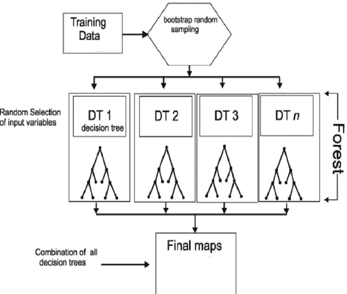
2. 6. Random Forest ... 35

2. 6. 1. Methodology of Random Forest ... 35

2. 6. 2. Application of Random Forest for detecting gene-gene interactions ... 37

2. 6. 3. Strengths of Random Forest ... 37

2. 6. 4. Weaknesses of Random Forest ... 37

3. Bayesian methods... 37

3. 1. Methodology of Bayesian methods ... 38

3. 2. Application of Bayesian methods in the detection of gene-gene interactions ... 38

3. 3. Strengths of the Bayesian methods ... 40

3. 4. Weaknesses of the Bayesian methods ... 40

Objectives ... 41

Experimental Section ... 43

Study 1: KNN-MDR: a learning approach for improving interactions mapping performances in genome wide association studies ... 44 Background ... 48 Methods ... 50 Results ... 56 Discussion ... 58 Conclusions ... 64 References ... 66

Study 2: Aggregation of experts: an application in the field of “interactomics” (detection of interactions on the basis of genomic data) ... 72

Background ... 76 Methods ... 77 Results ... 85 Discussion ... 93 Conclusions ... 96 References ... 98 Discussion - Perspectives ... 102 Conclusions ... 109 References ... 111

Appendices (Additional files) ... 119

Appendix 1 (Additional file 6): KNN MDR: user's guide ... 119

Appendix 2 (Additional file 7): Competitor methods ... 127

Appendix 3 (Additional file 8): Computing multi-locus penetrances. ... 129

Summary

Introduction

These last years have seen the emergence of a wealth of genetic information at the molecular level. Some of the main recent breakthroughs in biology originate from this new knowledge, allowing application of new strategies in many fields of the biological research. Although approaches targeting the association between phenotypic characteristics and DNA variations have been successful, many elements in the genetic landscape of the studied traits are still unknown and uncharacterized. A track to new findings, potentially useful for a better understanding of complex determinisms, is the detection of interactions between genomic regions affecting the traits of interest rather than single locus associations. While the detection of such interactions has been the focus of many methods, and despite some successes of these methods to solve difficult problems and to detect some of these genetic interactions, there is currently no gold standard method able to detect interactions in all situations, and the relative performances of these methods remain largely unclear. This thesis is a contribution to this field of interactions mapping:in the first study, we propose a novel approach combining K-Nearest Neighbors (KNN) and Multifactor Dimensionality Reduction (MDR) methods for the detection of gene-gene interactions as a possible alternative to existing algorithms, especially in situations where the number of involved determinants is high. In the second study, we propose another strategy based on the principle of the aggregation of experts, where the experts would be a set of popular published methods.

Results

The results obtained in the first study on both simulated data and real genome-wide data demonstrate some of the features that make KNN-MDR interesting in terms of accuracy and power: in many cases, it significantly outperforms its recent competitors. More specifically, the analyses on a real large dataset demonstrate the feasibility of scans using a large number of markers, as opposed to MDR where the computer burden explodes with the number of markers (when it simply increases linearly with KNN-MDR). This might for example allow highlighting interactions between markers far apart on the genomic map (trans-interactions), while some strategies propose to restrict the scans to close-by markers (cis-interactions) or to markers with significant marginal effects to reduce the amount of computations.

For the second study, we also show that aggregating methods results is a strategy with interesting features for detecting epistatic interactions. Experimental results, based again on simulated and real

genome-wide data, show that the aggregated predictor can produce better performances, in terms of statistical power and false positive rates, than each individual predictor to detect genetic interactions. It is consequently a useful addition to the various methods available to tackle this complicated problem.

Conclusion and Perspectives

In this dissertation, we focused on investigating and developing non-parametric statistical methods aiming at the detection of genetic interactions. We have shown that our novel methods complement, and sometimes improve, existing approaches used to detect genetic interactions in simulated and real datasets. The presented methodologies (KNN-MDR and aggregation of experts) are valuable in the context of loci and interaction mapping and can enhance the understanding of the biological mechanism underlying traits of interest, including diseases. More precisely, the new knowledge gained using these methodologies can assist in the prediction of clinical diseases and can contribute to provide new therapeutic opportunities.

To take further steps to these appealing perspectives, a first objective could be to implement a better version of the KNN-MDR software. The improvements could be on the overall performance of the software (optimization of the time-consuming parts of the program, parallelization), but also on the improvement of the “user-friendliness” of the program. This would involve an easier (and maybe automated) tuning of the parameters allowing an optimal detection power. These parameters include: the optimal sizes of the windows - which are dependent on the studied population, the markers density, the LD pattern, the optimal size of the neighborhoods to be considered, the pre-selection of markers in the early phase of large dataset analyses, the used distance measure or the adaptative selection scheme for the selection of markers in large studies, among others, the use of other types of genomic variants (microsatellites, copy number variations, sequencing data).

Another potential track would be to use a priori information on the interactions: this could be by using the results of previous studies, or by exploiting the known information on gene networks.

Résumé

Introduction

Ces dernières années ont vu l'émergence de sources riches d'informations génétiques au niveau moléculaire. Certaines des principales percées récentes en biologie proviennent de ces nouvelles connaissances, permettant l'application de nouvelles stratégies dans de nombreux domaines de la recherche biologique. Bien que les approches ciblant l'association entre les caractéristiques phénotypiques et les variations de l'ADN aient été couronnées de succès, de nombreux éléments dans le paysage génétique des caractères étudiés sont encore inconnus et non caractérisés. Une piste potentielle vers de nouvelles découvertes, qui pourrait aider à mieux comprendre les déterminismes complexes, est de détecter les interactions entre les régions plutôt que les associations avec une région unique. Alors que de nombreuses méthodes ont été proposées pour détecter de telles interactions et malgré le succès de ces méthodes pour résoudre certains problèmes et détecter certaines de ces interactions génétiques, il n'existe actuellement aucune méthode de référence capable de détecter les interactions dans toutes les situations. De plus, les méthodes restent relativement peu efficaces. Cette thèse est une contribution au développement de méthodes dans ce domaine.

Dans la première étude, nous proposons une nouvelle approche combinant les méthodes des K Plus Proches Voisins (KNN) et de Réduction Multidimensionnelle (MDR) pour détecter les interactions entre régions génomiques comme alternative possible aux algorithmes existants, notamment dans les situations où le nombre de déterminants impliqués est plus élevé que deux. Dans la deuxième étude, nous proposons une stratégie basée sur le principe de l'agrégation d'experts, où les experts seraient différentes méthodes de détection d’interactions validées et publiées dans des revues scientifiques.

Résultats

Les résultats obtenus dans la première étude à la fois sur des données générées par simulation et sur des données réelles à l'échelle du génome démontrent certaines des caractéristiques qui rendent l’application du modèle KNN-MDR potentiellement intéressante en matière de précision et de puissance : dans de nombreux cas, il surclasse nettement ses concurrents. De plus, des analyses sur un large ensemble de données réelles démontrent la faisabilité d'analyses utilisant un grand nombre de marqueurs, par opposition à la méthode MDR où la charge informatique explose avec le nombre de marqueurs (alors qu’elle augmente simplement linéairement avec KNN-MDR). Cela pourrait par exemple permettre de mettre en évidence des interactions entre des marqueurs éloignés sur la carte génomique alors que certaines stratégies proposent de limiter les scans aux marqueurs proches ou à un ensemble de marqueurs préalablement sélectionné pour réduire la quantité de calculs.

Pour la seconde étude, nous montrons aussi que la méthode de l'agrégation des résultats est une stratégie avec des caractéristiques intéressantes pour détecter les interactions épistatiques. Les résultats expérimentaux, basés à nouveau sur des données simulées et réelles à l'échelle du génome, montrent que le prédicteur agrégé peut produire de meilleures performances que chaque prédicteur individuel pour détecter des interactions génétiques, et est donc un complément utile aux diverses méthodes disponibles pour résoudre ce problème compliqué.

Conclusions et Perspectives

Dans cette thèse, nous nous sommes concentrés sur l'étude et le développement de méthodes statistiques non paramétriques pour la détection des interactions génétiques. Les méthodes que nous proposons sont présentées pour compléter et améliorer les approches existantes utilisées pour détecter les interactions génétiques dans des ensembles de données réelles et simulées. Les méthodologies présentées (KNN-MDR et agrégation d'experts) sont utiles dans le contexte de la cartographie des interactions et peuvent améliorer la compréhension du mécanisme biologique sous-jacent à divers caractères d'intérêt, y compris des maladies. L’acquisition de cette nouvelle connaissance, outre la compréhension fondamentale qu’elle implique, peut par exemple contribuer à la prédiction pronostique ou diagnostique des maladies étudiées, peut offrir de nouvelles possibilités thérapeutiques ou peut conduire à l’amélioration de caractères ayant un intérêt médical, agronomique, zootechnique ou autre.

Pour aller plus loin par rapport à ces perspectives attrayantes, un premier objectif pourrait être de mettre en œuvre une meilleure version du logiciel KNN-MDR. Les améliorations pourraient porter sur la performance globale du logiciel (optimisation des parties chronophages du programme, parallélisation), mais aussi sur l'amélioration de la "convivialité" du programme. Cela impliquerait un réglage plus facile (et peut-être automatisé) des paramètres permettant une puissance de détection optimale. Ces paramètres comprennent: les tailles optimales des fenêtres - qui dépendent de la population étudiée, la densité des marqueurs, le modèle de LD, la taille optimale des voisins à considérer, la présélection des marqueurs dans la première phase des analyses de grands ensemble de données, la mesure de la distance utilisée ou le schéma de sélection adaptatif pour la sélection des marqueurs dans les grandes études, entre autres, l'utilisation d'autres types de variantes génomiques (microsatellites, variations du nombre de copies, données de séquençage).

Une autre piste potentielle serait d'utiliser des informations sur les interactions: cela pourrait être possible en utilisant les résultats d'études antérieures, ou en exploitant les informations connues sur les réseaux de gènes.

Genetics laboratories activities have recently become more familiar in the public audience: forensics and DNA profiling are present in many prime-time shows and series, and genetic diseases research is nowadays largely advertised and sometimes supported through crowdfunding. The recent increase in the public interest for this science somehow reflects the huge advances made in genetics in the recent decades. Genetic technologies have indeed revolutionized our ability to explore the genetic architecture underlying complex traits and generated high (and sometimes exaggerated) hopes to understand the fundamental molecular mechanisms underlying biological processes, such as solving medical problems or improving the efficiency of bio-mechanisms underlying traits of economic importance. One of the disciplines involved to reach these long-term perspectives is positional cloning of genes. The aim of this technique is to identify genomic regions underlying traits of interest based only on the phenotypes and the genotypes of individuals for a panel of molecular markers. In this field, breakthroughs in the genotyping and sequencing technologies - such as DNA markers microarrays and NGS techniques - have made association studies based on the whole genome affordable in many species and populations. This new situation of large molecular data availability was promising and expectations were high that many new insights would readily become available to scientists. Despite many successes in the last two decades, much work remains to be done. As an example of the progresses to be made, the genetic variants identified to date in most genome-wide association studies only explain a small part of the total heritability of the studied traits. Although other explanations are possible, genetic interactions (epistasis) is one potential important source of unexplained variability. Consequently, further investigations in the field of interactions mapping in large-scale studies seems a reasonable avenue of promising research. Our work is a contribution to this field.

Throughout this thesis work, we have aimed at presenting statistical non-parametric methods for identifying potentially epistatic interactions from genomic (and sometimes genome-wide) data. We have assessed the mechanisms and the main characteristics of these new methods and we have tried to provide some evidence for the utility of these methods over simulated and real data.

More specifically, in the first study, we propose a novel approach combining K-Nearest Neighbors (KNN) and Multifactor Dimensionality Reduction (MDR) methods for detecting gene-gene interactions. This method is an extension of the well-known MDR methodology. It increases the span of the possible situations where MDR can be useful to situations with large number of markers and when the number of underlying genetic determinants is potentially higher than two. The way we use the data in KNN-MDR is shown to have a positive impact on the computational burden, making accessible situations that could not be tackled using the classical MDR techniques. Furthermore, and as a side effect, the approach we propose is also shown to be more powerful and accurate in difficult situations where individual genes have only minor (or no) marginal effect and where genetic heterogeneity - i.e. different genotypic configurations leading to the same phenotype, and the same

genotype leading to distinct phenotypes - is present. A comparison of our method (KNN-MDR) to a set of the other most performing methods has been carried on to detect interactions using simulated data as well as real wide data. Experimental results on both simulated data and real genome-wide data show that KNN-MDR has, as mentioned, interesting properties in terms of accuracy and power, and that, in many cases, it performs better than its recent competitors.

In a second study, we propose using a method based on the principle of the aggregation of experts, where the experts would be a set of popular published methods. The rationale of the aggregation strategy we propose is to benefit from the synergistic work of known methods, each with different strengths and weaknesses, to produce more reliable results than each of these individual methods. Our work shows that this strategy might lead to increases in both detection power and accuracy in the genetic interactions problem, while properly controlling for false discoveries.

In summary, our contribution to the hunt for genomic interactions underlying phenotypic traits is to provide one non-parametric method and one strategy allowing to improve the detection characteristics, and to show how these approaches could be used on today large real datasets.

1. General introduction

These last years have seen the emergence of a wealth of biological information and a steep increase in the rate of development of genomic and other basic biological research. Facilitated access to the genome sequence, along with massive data on genes expression and on proteins have revolutionized the research in many fields of biology (Visscher et al. 2012). The development of efficient genomic tools has allowed unraveling a large share of the molecular variation in many species, paving the way for studies aiming at associating genomic polymorphisms to phenotypic variation. An instance of this process is the use of panels of single nucleotide polymorphisms (SNPs) in large scales studies to track genes potentially involved in complex traits such as human, animal or plant diseases, for example (Kadarmideen 2014). Molecular analyses are nowadays commonly performed to examine candidate genomic regions or even the whole genome (in so-called “genome-wide association studies” (GWAS)) for causative genomic variants (Katsanis et al. 2013). The knowledge of these influential regions is of particular interest, since they are likely to harbor important genes involved in the onset of the disease and provide clues to the underlying mechanisms. Although these analyses are progressively becoming widespread, and despite successes in studies targeting for example diabetes (Frau et al. 2017) or Crohn disease (Libioulle et al. 2007), a large part of the genetic landscape of most traits is still unknown and uncharacterized, with in many cases the tested genetic variation only explaining less than 5%-10% of the risk of the disease (Riancho 2012). (Visscher et al. 2012) (Korte et al. 2013) suggested that this low figure could be due to the presence of a large number of different genetic causes and to potential interactions between genes. Consequently, a deeper understanding of the genotype to phenotype relationships will necessitate much more work in many situations (Yee et al. 2016).

In this thesis, we have tried to elaborate methods aiming at discovering simultaneous factors acting on the onset of the disease as an alternative to methods targeting single regions. Although we have focused on genomic regions, such methods could also encompass situations where genes and environment interact to produce the observed phenotypes. The main reason for that choice is that many signs indicate that interactions of several genes to underlie many traits might be the rule rather than the exception (Stanislas et al. 2017). Firstly, from a purely biological point of view, most genes are involved in complex networks where they interact with other genes; changes (mutations) in one gene might have or not an impact on the behaviour of the network, and several simultaneous mutations might be necessary to change the products of the network. Consequently, many scenarios are possible, some of which suggesting epistatic interactions between genes (Zou et al. 2017). Second, from a more pragmatic point of view, the mapping effort using single regions, although sometimes successful, have often failed to demonstrate genotype to phenotype relationship. This might be due to a lack of statistical power, as has been suggested, or to a poorly specified model (or to both): due to

interactions, a gene might mask the effect of another gene, preventing to associate clearly this second gene to the studied phenotype (Jung et al. 2016). The next section illustrates this situation.

1.1. An example of interaction

Various mechanisms of interactions exist and examples of each of these mechanisms can be found in the genetic literature (Costanzo et al. 2016). We will use the “complementary gene action” to illustrate the principle and to explain the difficulties for gene mapping due to this determinism. A classic example of this type of interactions is the sweet pea flowers colour problem: when crossing two parental white coloured lines, researchers obtained a completely purple F1 line. Next, when generating the F2 line (i.e. crossing the F1 individuals), an unexpected ratio of 9:7 purple-coloured to white-coloured flowers is observed. The explanation is as follows:

The determinism involves two genes, with two alleles each, noted A and a for the first and B and b for the second.

The parental lines have (fixed homozygous) genotypes AAbb and aaBB, respectively. All F1 individuals are thus AaBb.

If the genes are on distinct chromosomes (or sufficiently far apart on the same chromosome), four types of gametes are equally likely: AB, Ab, aB and ab.

These 4 gametes lead to 16 equally likely genotypes in the F2 population, summarized in the following table:

AB Ab aB ab AB AABB AABb AbBB AaBb Ab AABb AAbb AaBb Aabb aB AaBB AaBb aaBB aaBb ab AaBb Aabb aaBb aabb

Table 1 - an example of interaction. Involved genes show a “complementary gene action”: both dominant alleles are needed to obtain one of the phenotypes (purple colour, here)

So, obtaining the purple color necessitates that both A and B alleles be simultaneously present. The underlying genes are said to be “complementary”. This type of behavior has strong consequences on mapping experiments: imagine that a set of flowers is collected and that purple and white plants are genotyped in order to identify the genomic regions involved in the color determinism. Mapping single regions would probably fail to identify the individual genes (for example, some AA plants are white, but some other AA plants are purple), while using 2 simultaneous regions would probably identify the 2 genes (all A-B- plants are purple, while all other genotypes lead to white flowers).

1.2. Definition of genetic interactions

A gene interaction is an interplay between multiple genes that has an impact on the expression of an organism's phenotype (Costanzo et al. 2016). In this work, we will only consider interactions between genes, although other types of interactions are possible, such as for example the dominance (interaction between the alleles of a single gene) or interactions between proteins. The term gene-gene interaction is also known as epistasis or genetic interaction (Moore et al. 2005). We showed above an example of interaction, but various other types are possible. Three well-known examples are:

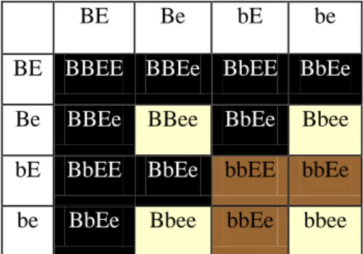
 Recessive epistasis: when the recessive allele of one gene masks the effects of either allele of the second gene (Marcelo et al. 2005). An example of this is the coat colour in Labrador retriever (Schmutz et al. 2007): one gene codes for pigment production (B) and the other for diffusion of the pigment into the air shaft (E). Mutations in E (e) leads to no diffusion of the pigment in the coat, no matter whether black (B) or brown (b) pigments were produced: all individuals carrying the recessive ee genotype will end up as golden coat. This is summarized in Table 2.

BE Be bE be BE BBEE BBEe BbEE BbEe

Be BBEe BBee BbEe Bbee bE BbEE BbEe bbEE bbEe be BbEe Bbee bbEe bbee

Table 2 - an example of recessive epistasis. The possible genotypes are displayed and the background colour corresponds to the dogs coat colour.

 Dominant epistasis: when the dominant allele of one gene masks the effects of either allele of the second gene (Marcelo et al. 2005). An example is the summer squash, where the colour of the plant is due to 2 genes. If the dominant allele of the second gene (B) is present, the squash will be white no matter the genotype at the first gene. If the genotype at the second gene is the recessive one (bb), then the colour will depend on the presence of the dominant allele at the first gene (A): homozygous (AA) or heterozygous (Aa) individuals will be yellow, while recessive homozygous (aa) plants will be green. This is summarized in Table 3.

AB Ab aB ab AB AABB AABb AaBB AaBb Ab AABb AAbb AaBb Aabb

aB AaBB AaBb aaBB aaBb ab AaBb Aabb aaBb aabb

Table 3 - an example of dominant epistasis. The possible genotypes are displayed and the background colour corresponds to the summer squash colour.

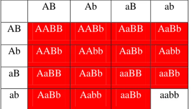
 Redundant genes: when a gene with a dominant allele is duplicated (and this is also true when genes are replicated several times), only double (multiple) recessive individuals will display the recessive phenotype (Nowak et al. 1997). An example is the snapdragon flower colour, which is red when a dominant allele is present, and white if not. This is shown in Table 4.

AB Ab aB ab AB AABB AABb AaBB AaBb

Ab AABb AAbb AaBb Aabb

aB AaBB AaBb aaBB aaBb

ab AaBb Aabb aaBb aabb

Table 4 - an example of redundant genes. The possible genotypes are displayed and the background colour corresponds to the plant flowers colour.

1.3. Is epistasis important?

There is a debate between those claiming that interactions contribute an important share to the genetic variation, and those who consider that the phenomenon is of minor importance to explain that variation. A first remark is that a distinction should be made between additive and total genetic variations (i.e. including non-additive effects, such as epistatic effects): the first leads to the so-called narrow-sense heritability where is the additive genetic variance and is the phenotypic variance, and where is the genetic variance due to non-additive effects (dominance, epistasis) (Mackay and Moore, 2014). Therefore, the relative importance of the non-additive variance in the genetic determinism of the traits is debated. In (Hill et al., 2008), it is argued that most of the genetic variation is additive. Since additive effects are transmitted from each of the parents to the descendants, while non-additive affects are not (they are rebuilt from the new combinations arising from the new combination of gametes), this is of course of special importance for breeders, who will mostly select on additive values. Nevertheless, other authors show that considering non-additive effects could improve prediction accuracy in situations where the underlying determinism is largely or partially due to epistatic interactions (Morgante et al., 2018), (Carlborg and Haley, 2004). For most complex traits, the determinism is largely unknown and the presence of epistatic interactions cannot be a priori discarded. Consequently, our view is that unravelling such interactions might contribute, in

variable proportions, to a better knowledge of complex traits. This view has been illustrated in the previous section.

1.4. Position of the problem.

As mentioned above, the massive amount of available molecular information did not allow, in many applications, to unravel the exact relationship between the genomic configuration, including the interactions between the involved genes, and the phenotypic expression (Fuxman Bass et al. 2016). The failure of “simple” association models led to try to associate observed variations at the macroscopic level (phenotype) to identified variations and their interactions at the molecular level (Hu et al. 2011).

This approach introduces at least two challenges:

1. the genetics underlying most traits of interest is complex and probably involves most of the time many genes and many interactions between these genes, leading to a complex relationship between genomic variants and phenotypes. Properly modelling such intricate network of genes and interactions is a potentially very challenging task. Consequently, identification of every (or even of any) interaction is a potentially very difficult aim.

2. from a more statistical point of view, fully modeling the underlying genetic complexity leads to models with large dimensionality, causing the well-known ‘curse of dimensionality’ problem: higher complexity corresponds to larger sets of parameters to estimate, to larger search spaces and to the need for huge collection of observations to efficiently scan these search spaces and accurately estimate the parameters with sufficient power.

In our work, we have investigated the use of non-parametric modelling as an alternative to parametric methods to solve these problems. One of the reasons under this choice is that many methods, described below, have been developed with some success using that approach. Another one is that the problems linked to the estimation of the parameters in parametric approaches could make these estimations less affordable in models involving interactions, and therefore render the use of such models more questionable (Ma et al. 2011).

Note nevertheless that increasing the number of parameters to be identified, although potentially making the power issues developed above even more critical, might also lead to more accurate models of the underlying genetics by introducing interactions (Maity et al. 2011). Better models of the underlying genetics might in turn improve the detection power of the effects of interest. Consequently, it is not necessarily obvious that interaction models will present poor power when compared to non-interaction ones, which should motivate more research on this subject.

1.5. Interest of the work

The knowledge of the relationship between variations at the molecular or cell level and phenotypic variation is of major importance from various points of view. It is of fundamental interest to understand how subtle molecular variations lead to various phenotypes and to be in a position to dissect complex mechanisms into small manageable pieces, allowing to cope with the inherent complexity underlying a trait of interest. Applied aspects are most of the time at least as important as fundamental ones: a better understanding of the genetic components and of the mechanisms leading to some diseases might give some keys to potential therapies, and the discoveries of molecular mechanisms at the root of quantitative traits of interest, such as pathogen resistance or animal production, might assist the breeders in the production of more robust and sustainable animals or plants.

1.6. Biological background

Unlike Mendelian diseases, in which disease phenotypes are largely driven by mutations in one or two gene loci, complex diseases such as rheumatoid arthritis and many cancers are influenced by a complex interplay of genetic and environmental factors (Quintana-Murci 2016). The examples provided above should have explained what makes the interacting factors hard to discern, and this gets of course even truer when the interacting genes are unknown.

Genome-wide association studies (GWAS), in which several hundred thousands to more than a million single nucleotide polymorphisms (SNPs) are assayed in thousands of individuals, represent a powerful tool to study the genetic architecture of complex diseases (Visscher et al. 2012). During the past few years, these studies have identified hundreds of genetic variants associated with complex diseases and have provided valuable insights into the complexities of their genetic architecture (Manolio et al. 2009). Nevertheless, most variants identified so far have been found to confer relatively small information about the relationship between the genomic variants and the phenotypes because of a lack of reproducibility of the findings, or because these variants most of the time explained only a small proportion of the underlying genetic variation (Fang et al. 2012). This observation has been quoted as the ‘missing heritability’ problem (Manolio, et al. 2009). Moreover, hundreds of studies have searched for gene-gene and gene-environment interaction effects in GWAS data with the underlying motivation of identifying or at least accounting for potential biological interactions. So far, this quest has been mostly unsuccessful (Aschard 2015). We therefore developed statistical methods to contribute to address this problem.

1.6.1. Molecular markers

Genetic mapping models rest on molecular markers to serve as proxies of neighbouring genes: detected significant interactions between markers will be interpreted as potential interactions between

genes close to these markers (Moore et al. 2005). In this context, “close to a marker” means “in linkage disequilibrium (LD) with the marker” (although other reasons, such as genetic drift or selection, might also lead to LD without the need for the gene and the associated markers to be physically close). Any DNA polymorphism is eligible as a molecular marker. This includes microsatellites, copy number variations, insertions/deletions, single nucleotide polymorphisms, among others. We next describe a few of these polymorphisms.

1.6.1.1. Single nucleotide polymorphisms

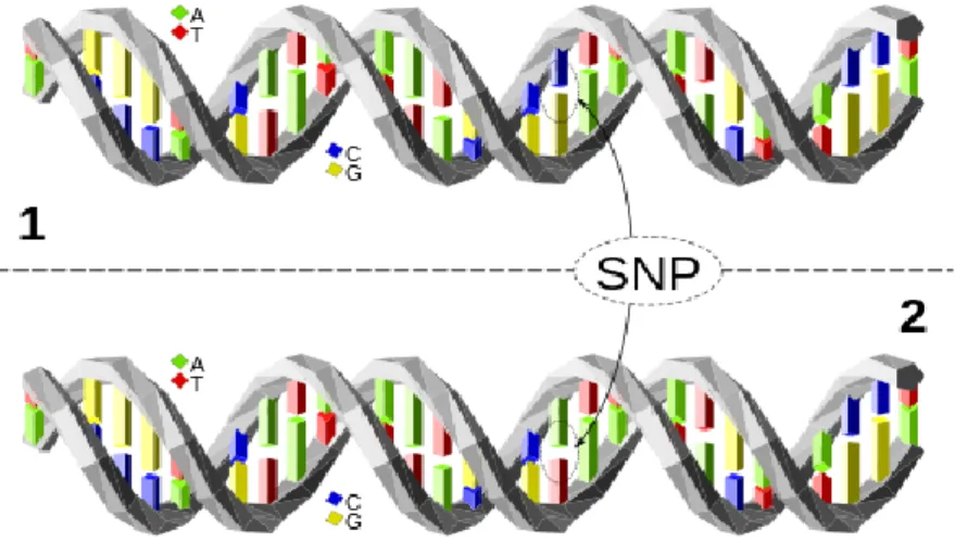
A single nucleotide polymorphism, or SNP (pronounced "snip"), is a variation at a single nucleotide position in a DNA sequence, as exemplified in Figure 1: the DNA sequences in the 2 pieces of DNA are identical except for a nucleotide, where they differ. Most SNP are biallelic, with a vast majority exhibiting either C/T alleles or A/G alleles. These distinct alleles can be present in a single individual (making this individual heterozygous for the SNP) and/or throughout the population. The frequency of the minor allele (the less frequent one) varies from SNP to SNP, with values ranging from close to 0 % up to values close to 50 %. On average, human DNA consists of a SNP for every 300 bases, meaning that, for the whole genome (3 billion bases), there would be roughly 10 million SNPs (Liu et al. 2015).

Figure 1 - a SNP. The two molecules of DNA only differ at one nucleotide

1.6.1.2. Microsatellites

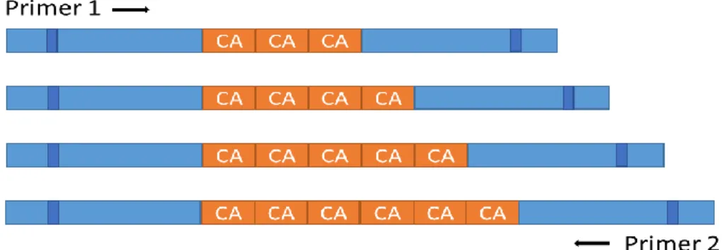
A microsatellite, or Single Sequence Repeats (SSRs), is a group of repetitive DNA in which certain DNA motifs (1 to 10 nucleotides) are repeated, typically 5–50 times. They tend to occur at thousands of locations within an organism's genome. They have also a higher mutation rate and a higher genetic diversity than other areas of DNA, which makes them a good candidate as a genetic marker (Vieira et al. 2016).

Figure 2 - a microsatellite marker. The number of copies of the CA nucleotides tandem varies from copy to copy.

1.6.1.2. CNV (Copy Number Variations)

A copy number variation is a phenomenon in which large regions of the genomes are either duplicated or deleted, creating structural variant regions. The supplementary copies can involve fairly large stretches of DNA (sometimes thousands of nucleotides). The regions with such variations cover a relatively large portion of the genome (up to 10% of the human genome, for example) (Thapar et al. 2013). These structural variants provide a support for the evolution of genes to new functions, but can also be causative of disease.

Figure 3 - a Copy Number Variation.

1.4.1.2. Insertions and deletions (INDELs)

Small insertions or deletions - commonly called INDELs - are another important source of genetic polymorphisms. In terms of base pairs of variations, INDELs cause similar levels of variation as SNPs (Mullaney et al. 2010).

Figure 4 - INDELs. Using the first sequence as a reference (“wild type”) sequence, 3 base pairs (AAA, in blue) have been deleted in the second sequence (deletion), and 4 base pairs (TGTG, in red) have

been inserted in the third sequence.

1.7. Statistical background

A statistical model is an attempt to provide a mathematical abstraction of the mechanisms that produced the observations. The model makes some assumptions and some simplifications of the reality in order to make things still manageable in terms of the involved mathematics and of the computing burden while still providing a hopefully useful view of the studied phenomenon (Calzone et al. 2015). The goal is to be able to properly describe the state of nature and to make accurate predictions. In our mapping context, the models should be able to identify pieces of the genome that are involved in the studied trait. Although several taxonomies exist for the models, we will concentrate in the following paragraph on the distinction between parametric and non-parametric models, which is important to describe our work.

1.7.1. Parametric models

A parametric model is a family of distributions such that each member of the family can be described using a finite set of parameters and all the parameters are in finite-dimensional parameter spaces. An example of such families is the normal family, indexed by the 2 parameters µ (the mean, which is also the expected value of the modeled variable) and (the standard deviation, the squared root of the expected squared distance to the mean). The classical normal distribution formula:

where µ can take any real value and can take any positive value, thus defines a family of distributions, used to model a variable (and, more generally, a set of variables) assumed to originate from the well-known bell-shaped distribution. Such models are widely used, including in the field of genetic mapping. Most common applications targeting genes and quantitative trait loci mapping strategies include linear regression, logistic regression, classical and generalized mixed models, among others (Howard et al. 2014).

Common features of parametric models are:

 They perform correctly with relatively small dataset and can avoid overfitting due to the a priori imposed structure (Sun et al. 2017).

 They are optimal (“best”) when correct parameters are chosen (Elster et al. 2005).

 Although they make stronger assumptions about the data, they work well if the assumptions are correct (Goodrich 2012).

These models generate several statistical challenges. For example, in the “genomic selection” procedures, the phenotypes of interest are modeled as a sum of marker effects added to a sum of other (non-genetic) effects. Since many markers (p) are available on a restricted set of (n) individuals, leading to much more unknown than data points, techniques such as the LASSO (Least Absolute Shrinkage and Selection Operator) or Bayesian techniques must be used to solve such problem, leading to more difficult interpretation of the effects of the variables (Howard et al. 2014). Another challenge is that traditional parametric methods need strong model assumptions to model interactions, such as assuming linear G×G interaction. This assumption, however, could be easily violated due to the underlying nonlinear machinery between the genetic factors. As mentioned above, misspecification in parametric models could lead to large bias (Ma et al. 2011, Maity et al. 2011).

1.7.2. Non-parametric models

Unlike parametric models, non-parametric models are not based on parameterized families of probability distributions. Nonparametric statistics make no assumptions about the probability distributions of the variables being assessed, and they can take big dimensional parameter spaces (Li et al. 2013).

In short, in non-parametric models:

 The data is summarized using an unknown set of parameters (Hamilton et al. 2017).

 Some of the original data must be kept to make predictions or to update the model (Ghahramani 2012).

 No assumption is made about probability distributions (Ghahramani 2012).

 Models are generally slower, but potentially more accurate, especially when the assumptions made in parametric models are questionable (Ho et al. 2017).

In the interaction mapping field, many non-parametric methods have been devised (Support Vector Machine, Neural Networks, Random Forest, k-nearest neighbors algorithms, ...). These nonparametric models have the potential to bring new solutions for the challenges in the domain (Gianola et al. 2006) because of their ability to handling multiple genetic variants with the consideration of possible high-order G-G interactions, and because they do not make any assumption on the disease models (Li et al. 2013, Howard et al. 2014, Li et al. 2014).

1.7.3. Modelling interactions

The regulatory interactions in genetic networks form a complicated system and an important objective of systems biology is to model and infer these interactions. Proper modeling and inference of these genetic interactions requires understanding of the distinction between biological and statistical interactions (Forsberg et al. 2017).

1.7.3.1. Statistical interactions

The most common statistical definition of interaction relies on the concept of a linear model describing the relationship between some outcome variable and some predictor variable(s). The case of statistical interaction potential arises when there are two or more independent variables. The simplest case is when the effect of each independent variable is completely separate from the other independent variables. In this “no interaction” setting, the effects of the different independent variables act just additively. A more complicated situation arises when the effect of one independent variable depends on other independent variable(s). This is referred to as an "interaction" situation (Moore et al. 2005, Cordell 2009). Since, in this context, the effect of a variable cannot be obtained without considering other potentially interacting variables, it turns out that this situation can significantly complicate certain types of multivariate analyses with respect to situations where variables are assumed to be independent of each other (Yi 2010).

1.7.3.2. Biological interactions

Examples of biological interactions have been presented in a previous section. In our genetic mapping context, biological interactions mean in the widest sense the effect of a particular genotype on the phenotype depends on the genetic background. It can be defined in a simple, as the phenotypic effect of one locus depends on the genotype at the second locus (Carlborg and Haley, 2004). Also, it can be defined in a general, as the effect of a gene on a phenotype is dependent on the configuration of one or more other genes (Moore et al. 2005). In this context, many epistasis were detected as responsible for differences in phenotype such as comb type in chickens and coat color in various animals (Carlborg and Haley, 2004).

2. Use of non-parametric statistical methods in genetic interaction mapping applications

Various non-parametric methods have been used in genetic problems. In this section, we will review some of the most important methods in this field. Although notations in the following descriptions are mostly borrowed from the papers at the roots of the described methods, the data structures used by the methods are similar:

A set (ranging from a few hundreds to a few thousands, in most situations) of observations, each observation corresponding to a subject (human, animal or plant) used in the experiment. For each subject (i.e. observation), we have at least:

o A phenotype, to be seen as the dependent variable of interest. This phenotype, measured on the subject, can either be discrete (as, for example, in case-controls experiments, where the phenotype is either 0 (control) or 1 (case)) or continuous (blood pressure, or annual milk yield, for example).

o Genotypes, to be considered as the putative explaining variables. These genotypes have been obtained from the laboratory based on DNA samples originating from the subjects of the experiment. These genotypes are coded as discrete values representing the various possible genotypic configurations. For example, a SNP genotype could be coded as 0, 1 or 2 to represent the various possible genotypes (AA, AB or BB) for that SNP. The number of genotypes, typically corresponding to the number of markers used in the experiment, is generally large (from a few dozens to a few millions) and, in most situations, larger than the number of subjects.

One of the goals of the experiment is then to try to identify the set of genotypes with a significant impact on the studied .phenotype.

2.1. Support Vector Machines

Support vector machines (SVMs) are supervised non-parametric statistical learning techniques that analyze data and recognize patterns. They are used for classification and regression analyses. There is no assumption made on the underlying data distribution, which is utilizing hyperplanes in high dimensional spaces (Mountrakis et al. 2011).

2.1. 1. Methodology of Support Vector Machine

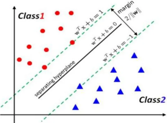
Let us assume an input (features) - output (classes) process producing paired data where is a pdimensional vector of features measured on a sample, that has been classified into a class (coded -1 or -1) represented by , . The training process of a (linear) support vector machine aims to find a linear separating hyperplane with the maximal margin (2 , the distance between and ) under the classification conditions:

Figure 5 - Linear SVM with maximum-margin hyperplane (Agrawal, et al., 2012).

In Figure 5, a hyperplane separates the two classes of input, where is the normal vector, is the bias, and “ ” is the dot product (Chen et al. 2008) (Koo et al. 2013).

Two additional hyperplanes separate the data from the previous hyperplane (defined by ) with no data between them. The additional hyperplanes are located at a maximum distance (known as margin) from the separating hyperplane. These hyperplanes have equations and , and are such that all points for which are from the first class and those for which are from the second class.

Furthermore, in Figure 5, the distance between two hyperplanes is equal to , and the offset of the separating hyperplane from the origin along the normal vector is determined by . Overall equation for the additional hyperplane can be written as

When the data points clouds overlap, a solution is to map the input vector data into higher dimensional space, known as the feature space, so that the linear separation can be achieved within that space (Koo et al. 2013).

SVM can also be extended to non-linear separating hyper surfaces using “the kernel trick”: the original input space is mapped into a high dimension space (the feature space) using a kernel function that is defined as where is kernel function that map input space into feature space (Sheng et al. 2014) and SVM is applied to these transformed couples.

Several kernel functions have been proposed in SVM to obtain the optimal solution; the most frequently used such kernel functions are (linear kernel is the simplest kernel function, given by the inner product (x,y)), (polynomial kernel is a

non-stationary kernel that it is well suited for problems where all the training data is normalized and where (the polynomial degree) and are kernel parameters (Chen et al. 2008) and (Sheng et al. 2014)), and (radial basis function)).

2.1.2. Application of Support Vector Machines to the detection of gene-gene interactions

SVM have been used to predict genetic interactions, which can be learned from the features of known genetically interacting pairs in order to predict which other pairs genetically interact.

In order to achieve this, the training data consists of two sets of features vectors, each set labelled as either positive (corresponding to the presence of genetic interaction) or negative (corresponding to the lack of genetic interaction). Each features vector characterizes a pair of genes rather than a single gene. When the features are mapped into a high-dimensional space, the SVM constructs a separating hyperplane that maximizes the margin between the features of genetically or not genetically interacting pairs. For this mapping, (Koo et al. 2013) used kernel function such as polynomial or radial basis.

In (Fang and Chiu, 2012), the authors have proposed an extended SVM method and a SVM based pedigree-based generalized multifactor dimensionality (PGMDR) for detecting gene-gene interactions in the absence or presence of the main effects of genes with an adjustment for covariates and on a limited sample of families. The results show that the proposed approaches of SVM and SVM-based PGMDR have higher power than other methods (PGMDR and FAM-MDR (family-based multifactor dimensionality reduction)) used for comparisons. In addition, although more computationally expensive than the other methods, these methods show higher prediction accuracy and power, making them valuable for the interactions detection problem.

In (Fang et al. 2013), the authors have also developed a novel approach named "backward support vector machine (BSVM)-based variant selection procedure" to identify informative disease-associated rare variants. The idea of this approach is that the rare variants are weighted and selected according to their positive or negative associations with the disease. The results on both simulated and real data show that the proposed BSVM approach is more powerful than the other approaches used in this study (such as set Kernel Association Test (SKAT)) .

In (Chen et al. 2008), the authors have also proposed SVM methods in various situations to detect gene-gene interactions and compared this approach to MDR (MDR is described below). The results show that SVM methods are a useful tool for the identification and characterization of high order gene-gene and gene-environment interactions but is computationally more costly than MDR.

2.1. 3. Strengths of Support Vector Machine

(i) SVM can deal with high dimension data set (Upstill-Goddard et al. 2013).

(iii) SVM is robust to noise and not prone to overfitting (Ozgur et al. 2008).

2.1. 4. Weaknesses of Support Vector Machine

(i) SVM is restricted to pairwise classification (Chen et al. 2008).

(ii) SVM cannot be directly used for features selection (Mountrakis et al. 2011).

(iii) The power of SVM might be reduced in the presence of genetic heterogeneity (Chen et al. 2008).

(iv) Computationally intensive (Wang et al. 2008).

2.2. Neural Networks

Another computational approach proposed for the study of disease susceptibility genes is neural networks (NN). Neural Networks are a class of pattern recognition methods developed in the 1940's to model the neuron, the basic functional unit of the brain. Neural networks process information in a way similar to the human brain. It consists of a large number of highly interconnected processing units (neurons) working in parallel to solve a specific problem (Motsinger-Reif et al. 2008).

2.2. 1. Methodology of Neural Networks

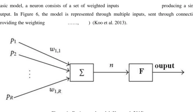
Single neuron model (also known as perceptron) is the basic neural model in neural networks. In this basic model, a neuron consists of a set of weighted inputs producing a single output. In Figure 6, the model is represented through multiple inputs, sent through connections providing the weighting ……, ) (Koo et al. 2013).

Figure 6 - Basic neural model (Koo et al. 2013).

The generated output is computed in two steps. A weighted sum of the inputs is first calculated using: (1)

Next, the weighted sum is compared to a threshold. For example, a F(x) Heaviside activation function is used when the weighted sum of inputs is compared to a null threshold, where F(x) is defined as

(2)

The perceptron, classifying individuals (represented by an input vector) into an output class (0 or 1 in the example given above), can serve as the basic building block for an artificial neural network (ANN), which is a more general classifier

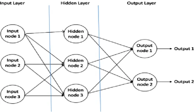
As a simple example of ANN, a feed-forward network was the first type of used artificial neural network. It contains multiple neurons (perceptrons) arranged in layers. Perceptrons from adjacent layers have connections or edges between them Figure 7. All these connections have weights associated with them (Konomi et al. 2017).

Figure 7 - An example of feedforward neural network.

From Figure 7, the outputs from the input layer are used as inputs for each node in the hidden layer. Similarly, the outputs of the nodes in the intermediate layer(s) serve as inputs for the next layer, propagating the signal down to the output layer. Classically, multilayer ANN consist of three layers or more, including an input layer, an output layer, and one or more hidden layers. Each node in one layer connects with varying weights to every node in the following layer, and the transfer function F(x) is very commonly a sigmoid function. Note that in the example presented here, the information moves in only one direction (feed forward). No cycle sending information from outputs to previous layers of the neural network is included.

2.2. 2. Application of Neural Networks in the detection of gene-gene interactions

Neural network methods are used to identify disease susceptibility genes in both linkage and association analyses. Although both types of analyses have the same objective - i.e. identifying

markers significantly associated to loci involved in the trait of interest -, the approaches differ: in linkage analysis, information from the pedigree and from the genotypes is used to follow the segregation of the trait in the pedigree and detect associations between the genotypes and the trait. In association analyses, this link is sought using individuals randomly sampled from the investigated population, and no pedigree is used. In disease mapping experiments, the sampling is stratified and samples are collected in cases and controls sub-populations (Curtis 2007). A consequence is that regions detected using association analyses are generally smaller than those detected using linkage analyses, but require denser markers maps. In general, in the genetic mapping context, the genotypes serve as input and the phenotype is the output of the neural network (Koo et al. 2013).

Various coding schemes are possible for the inputs and output of ANN. For example, the inputs can be the presence or absence of a specific marker allele (a value of 1 would represent the presence of the allele, and a value of 0 an absence of the allele).Another common encoding strategy for the inputs of a neural network is to use identity-by-descent (IBD) status of the genotypes: variable is set to 1 when the alleles in a genotype are supposed to be IBD, to −1 when not and to 0 when the genotype is uninformative. On the other side, several coding are also possible for the outputs of neural networks. For example, the output could be the disease status, in which a value of 1 would represent a case whereas a value of 0 would indicate a control (Motsinger-Reif et al. 2008).

In (Tomita et al. 2011), the authors have proposed artificial neural networks (ANN) for the detection of gene-gene interactions. The idea of this study is based on the use of artificial neural networks with the parameters decreasing method (PDM). The procedure of PDM begins by excluding one SNP from the total number of SNPs and constructs a model containing the remaining SNPs. In turn, each SNP is deleted from the total number of SNPs and with the remaining SNPs a model is constructed. The results demonstrate that the artificial neural network approach had more power than logistic regression (LR) to characterize the development of complex diseases such as an allergic disease.

In (Gunther et al. 2009), the authors have also proposed neural networks for the detection and the modelling of various types of gene-gene interactions. In their study, the authors used feed-forward multilayer perceptron (MLP) as a neural network, given that this method is able to approximate arbitrary functional relationships between covariates and response variables. The results on simulation data demonstrate that neural networks have more ability to detect and model different types of biological gene-gene interactions than others methods (logistic regression and MDR) which were used for comparison in the study.

2.2. 3. Strengths of Neural Networks

(i) NN are able to model the relationship between disease and single nucleotide polymorphism (SNP) (Tomita et al. 2011).

(ii) NN can make prediction on data where the disease outcome is unknown by learning the outcome given on a dataset (Basheer et al. 2000).

(iii) NN can deal with large volumes of data (Ritchie et al. 2003).

(iv) NN are still efficient in the presence of genetic heterogeneity, high phenocopy rates, polygenic inheritance, and incomplete penetrance (Motsinger-Reif et al. 2008).

2.2. 4. Weaknesses of Neural Networks

(i) NN work as a black box (Motsinger-Reif et al. 2008).

(ii) Difficult to list out all possible NN architectures, which causes the difficulty to find the optimal architecture (Basheer et al. 2000).

(iii) Result of NN are hard to interpret due to the dimensionality problem (Ritchie et al. 2003) (Curtis 2007).

2.3. Multifactor Dimensionality Reduction

MDR has enjoyed great popularity in the field of interaction mapping and a vast amount of extensions and modifications of the original method (Ritchie et al. 2001) have been suggested and applied, building on the general idea (Gola et al. 2015). It is a data mining approach for detecting and characterizing combinations of attributes or independent variables that interact to influence a dependent or class variable (complex gene–gene and gene–environment interactions) (Martin et al. 2006). The MDR method is nonparametric (i.e., no hypothesis about the distribution of statistical parameters is made), is model-free (i.e., it assumes no particular inheritance model), and is directly applicable to case-control and discordant-sib-pair studies (Manuguerra et al. 2007).

2.3. 1. Methodology of Multifactor Dimensionality Reduction

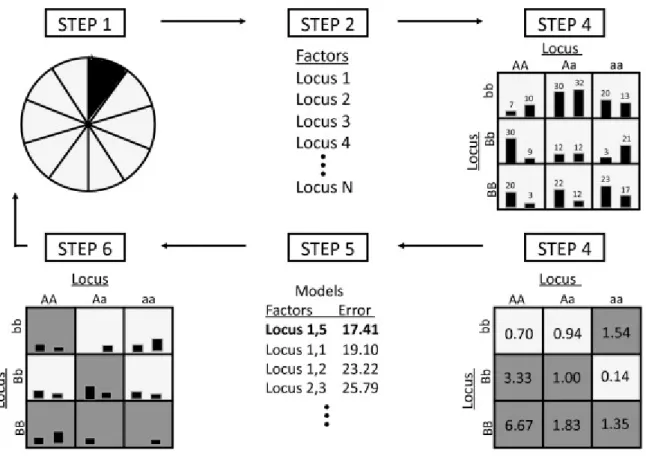
Figure 8 demonstrates the process for the MDR algorithm. Before the MDR analysis begins, the data set is divided into multiple partitions for cross-validation. Cross-validation is an important part of the MDR method, as it aims to find a model that not only fits the given data, but can also predict on future, unseen data (Ritchie et al. 2006).

Figure 8 - Steps of the MDR (Motsinger-Reif, 2008)

A summary of the general steps needed to implement the MDR method detailed in (Ritchie et al. 2006) are as follows:

1. In step one, the data is divided into k (typically, 10) random subsets. (k-1) of the subsets make up the “training set” while the last subset becomes the “testing set” (see also step 6, “cross-validation”).

2. In step two, a set of f factors is then selected from the pool of all factors. These factors can include both genetic and environmental data. There is no predefined limit on the number of independent variables that can be examined. However, limits due to computation time may arise, especially when the number of potential factors is high. For example, in genetic interactions mapping problems, if m markers are used, the number of possible configurations that could be tested is of the order of mf. Since m could easily be from several thousands to several millions in today applications, the search space can become intractable for values of f larger than 2 or 3. In Figure 8, f is equal to 2.

3. In step three, the f factors and their possible multifactor cells are represented in f-dimensional space, with all possible multifactorial combinations represented as cells in the table. The number of cases and controls for each locus combination are counted.

4. In step four, each multifactor cell in the n-dimensional space is labelled as high risk if the ratio of affected individuals to unaffected individuals exceeds a threshold of one (dark grey background cells), and low risk if the threshold is not exceeded (light grey background cells).

5. In steps five and six, the classification performances are estimated using the “testing set” data for each of the tested set of f factors.

6. The six steps are repeated using the k possible partitions of the original dataset into “training” and “test” sets.

7. The model with the best average performances is selected and the prediction error of the model is estimated using the independent test data.

Commonly, the classification performances are assessed using a ”balanced accuracy” criterion where the balanced accuracy is computed as a simple average of the sensibility and the sensitivity of the classifier. Repeating this procedure over all possible markers sets allows obtaining the best model, which is defined as the set of markers providing the best allocation performances. Significance for the optimal model can be obtained through a permutations test, in which the potential links between the individuals’ genotypes and the phenotypes are disrupted by randomly shuffling the phenotypes. The p-values obtained using this test have then to be corrected for multiple testing, where multiple tests are due to the number of models that are successively tested.

2.3. 2. Application of Multifactor Dimensionality Reduction to the detection of gene-gene interactions

A lot of applications use the principles of MDR, only a few of them will be mentioned below.

In (Calle et al. 2008), the authors have proposed a novel approach of MDR named “Model-Based Multifactor Dimensionality Reduction (MB-MDR)”. MB-MDR aims at identifying specific multi-locus genotypes associated with a disease susceptibility while allowing to adjust for marginal effects and confounders. Another difference between MB-MDR and MDR is that just those cells exhibiting significant evidence of (high or low) risk will be merged. The other cells which either show no evidence of association or have no sufficient sample size are included in an additional category, that of no evidence of risk. The results show that MB-MDR has improved power over MDR in the presence of genetic heterogeneity.

In (Cattaert et al. 2010), the authors have proposed an approach named “FAMily Multifactor Dimensionality Reduction (FAM-MDR)” for detecting gene-gene interactions. This method combines features from the genome-wide rapid association using mixed model and regression approach (GRAMMAR) (Aulchenko et al. 2007) with the approach (MB-MDR). The applications of this approach are on continuous traits, however it can be used for any type of binary traits. The result shows that FAM-MDR has improved power over the approach Pedigree-based Generalized MDR (PGMDR) in most of the simulations using continuous traits.

In (Yang et al. 2013), the authors have also proposed balancing functions for adjusting the ratio in risk classes and classification errors for Imbalanced cases and controls using multifactor dimensionality reduction (MDR-ER) as a novel method to improve MDR. The difference between MDR-ER and