Advantages of a semi-analytical approach for the analysis of an
evolving structure with contacts
V. Denoël∗
SUMMARY
This paper presents a semi-analytical approach for the evolution analysis of a beam into given boundaries. The analytical description of contact locations, contact forces and beam deflections results in an exact modelling of the phenomenon (no penetration allowed). Despite the apparent
complexity of the problem, the analytical relations leading to two-point boundary and integro-restrained differential equations are formally written. An iterative resolution of these equations is adopted by converting the problem into a single-point boundary value one. Due to a proper selection of the global unknowns, namely the contact forces and their locations, the proposed method is particularly efficient in the context of evolving structures. The resolution is illustrated on a simple example and comparisons with the finite element method are given as persuasive arguments.
key words: evolving structure, semi-analytical, contact, penetration
Postdoctoral Researcher, Fund for Scientific Research University of Liège, ArGEnCo - MS2F
Departement of Architecture, Geology, Environment and Construction Chemin des Chevreuils, 1, B52/3 - B-4000 Liège, Belgium
-Temporary invited scientist at the CSIRO,
Commonwealth Scientific and Industrial Research Organisation Dick Perry Avenue, 26, 6151 Kensington, Western Australia
1. INTRODUCTION
The insertion of a flexible beam-like object into a curved hollow cylindrical object is a basic problem encountered in many every-day applications. Many medical and bio-engineering operations require the introduction of a camera into the human body. Also, the endoscopic investigation of sewer nets requires the insertion of a flexible inspection system into the pipes. In other applications like the directional drilling of oil and petroleum wells, the reservoirs may have to be reached with curved trajectories ([1]). Another unusual application of this simple
∗Correspondence to: V. Denoël, University of Liège, ArGEnCo MS2F,Chemin des Chevreuils, 1, B52/3
-B-4000 Liège, Belgium
Contract/grant sponsor: National Fund for Scientific Research
problem concerns the introduction of a paper sheet into a toner ([2]). It is surprising to realize that this simple application is represented by a rigorous model whereas some applications in which people’s lives are at stake, like medical applications, usually rely on experience or specific experiments.
In these applications the inserted body presents generally a certain bending stiffness and at least an axial stiffness. As this paper aims at presenting a robust approach of the process, the beam is thus modelled according to the beam theory. It can be seen as a structure evolving into a pipe. The trajectory of its end depends on the medium in which it is introduced, the process (drilling, hammering, static penetration,...), the location of the contacts along the beam length and eventually the flexibility of the pipe walls. In many applications, the hollow cylindrical object, referred to as pipe in the following, can however be considered as rigid. If this is not the case, the analysis with assumed rigid walls is anyway enlightening because it represents a limit case with reduced beam-wall interactions.
In this paper, the shape of the pipe is supposed to be known beforehand and the main objective is the precise description of the contacts along the beam. Usually this problem is solved using the a finite element method ([3], [4]). Because the moving beam is inserted in a continuously deeper hole and because some localized details have to be represented precisely, the meshing of the beam into finite elements is not convenient. For this reason, a semi-analytical method is proposed for the analysis of the insertion of a beam into a given pipe. It is based on an analytical description of the large displacements of the beam and the contact locations. As a first advantage, no penetration is allowed because this condition is strictly and formally written. Furthermore, because it does not require any meshing, the resulting technique is particularly well adapted to model this evolving structure.
The major feature of the model lies in its enhanced description of the contacts. The contact positions and forces are the main scalar unknowns. As illustrated in section 3, they are computed by combining advanced numerical techniques, which justifies the semi-analytic character of the model.
The model is first presented on a simple application (section 3). Then the same problem is solved with the finite element method (section 4) and finally a numerical application is presented in order to compare both methods quantitatively (section 5).
2. General theoretical considerations
2.1. Beam theory
In the beam theory (e.g. [5]), under Bernoulli’s assumptions, the internal bending moment M and the shear force T are expressed by:
M = EIdΦ ds T = dM ds = EI d2Φ ds2 (1)
in which Φ is the slope of the beam with respect to a fixed direction, χ = dΦ/ds is the curvature and EI is the bending stiffness.
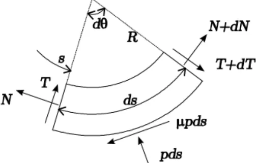
Figure 1. Elementary contact zone
2.2. Contact zones
Because the stressfree (initial) configuration of the beam is supposed to be straight, its insertion into a curved well necessarily implies contacts. Either these contacts are limited to usual point-like interactions represented by concentrated forces, either they involve a finite contact length along which the beam fits perfectly the boundary. In this latter case, the interaction consists of a varying pressure along the contact zone and two concentrated forces at both ends ([2]). Consideration of the equilibrium of an elementary contact zone (Fig. 1) results in:
pds + N dθ − dT = 0 ⇒ p = N R − dT ds (2) µpds − T dθ − dN = 0 ⇒ µp = TR+dN ds (3)
Because the beam is bent in order to strictly fit the boundary, its curvature is thus known in this zone. Equation (1) can be substituted into Eqs. (2) and (3), leading to a set of two equations with two unknowns, the reaction on the wall p(s) and the axial force N (s). A simple solution is obtained if there is no friction between the wall and the beam (µ = 0), if the contact zone is straight or circular (χ = χ0, R = R0), and if the beam has a uniform bending stiffness
(EI =constant ). In this case the axial force (N ) and the pressure (p = N/R) are both constant along the contact zone.
3. Semi-analytical approach
3.1. Governing equations
A semi-analytical approach is used for the computation of the quasi-static insertion of a beam into a given curved pipe. The method is illustrated on a simple application so as to enlighten clearly the advantages of the method. However it is worth noting that this semi-analytical approach can be applied to more complex problems.
The application consists in modelling the bending of a beam with a given length (L) inside a pipe composed of two straight parts linked by a curved one (Fig. 2). The pipe’s geometry is fully described by the length of the first straight part (D), the clearance (e/2), the radius
of curvature (R) and the angular opening (ϕ), which is also the slope of the second straight part. The beam is supposed to be hinged at the left end. At the other end, only a transverse reaction is considered in order to keep the beam end on the pipe axis. No external load is applied to this system and the deflections of the beam result therefore from the end reactions and the contact only.
During the insertion process, the beam end lies successively into the first straight part (Solution 1, not represented), into the curved part (Solutions 2 ) and finally into the second straight part (Solutions 3 ). A supplementary letter is added in order to distinguish the kind of contact. Only useful configurations for the forthcoming illustration are considered: no contact (a), a point-like contact (b), a continuous contact (c), two point-like contacts (d). A different set of governing equations has to be written and specialized for each configuration. In each case, the number of contacts and their nature are different. The scalar unknowns of the problem (reaction forces and locations) are thus different from case to case. Some configurations are represented in Fig. 2 with their corresponding unknowns.
Configurations 1, 2a and 3a lead to trivial equations: the slope of the deformed beam is constant and Eq. (1) indicates that internal forces are equal to zero. For the other configurations, at least one contact point (or zone) occurs and the deflections of the beam have to be computed: Eq. (1) has to be solved. Its solution is performed by decomposing the beam length [0; L] into contactless domains, limited by contact points or contact zones. For instance, configurations 2b, 3b, 2c and 3c are solved on two domains, one before and another one after the contact. The governing equations for these four configurations are presented in the following.
Basically the number of governing equations is equal to the number of domains, i.e. the number of contacts plus one (2 domains for configurations 2b, 3b, 2c and 3c). For the sake of compactness in the notations, bψ (the inclination of Q3),bs and bα (related to the beginning
of the second domain) are introduced. Depending on the considered configuration, and with notations of Fig. 2, they are equal to:
Solution 2b: ψ = α,b bs = s1,α = αb 1
Solution 2c: ψ = α,b bs = s2,α = αb 2
Solution 3b: ψ = ϕ,b bs = s1, bα = α1
Solution 3c: ψ = ϕ,b bs = s2, bα = α2 (4)
Thanks to these notations, the application of the beam theory (Eq. (1)) for the four considered configurations gives this common form:
s ∈ [0; s1[ → d2Φ 1 ds2 = Q0cos Φ1− N0sin Φ1 (5) s ∈ [bs; L] → d 2Φ 2 ds2 = −Q3cos ³ b ψ − Φ2 ´ (6)
where Φ1(s) and Φ2(s) represent the slope of the beam Φ (s) on each domain. These non-linear
second order differential equations require both two limit conditions to be solved:
Φ1(s1) = α1 and dΦ1 ds º s=0 = 0 (7) Φ2(bs) = bα and dΦ2 ds º s=L = 0 (8)
Figure 2. Examples of some considered configurations used to establish the governing equations
They correspond to tangency conditions at the contact and free moment conditions at the ends of the beam. The differential equations and their limit conditions (Eq. (5) to (8)) involve some complementary scalar unknowns: Q0, N0, Q3, s1, α1 and eventually some others among
s2, α2, α depending on the considered configuration. Some supplementary equations are thus
required. First the conservation of the axial force throughout the contact (see Section 2.2) is written:
Q0sin α1+ N0cos α1= Q3sin
³ b
ψ − bα´ (9)
Secondly the continuity of the curvature between the resolution domains is imposed. If the contact is localised (solutions 2b, 3b):
dΦ1 ds º s=s1 = dΦ2 ds º s=s1 (10)
and if the contact is continuous (solutions 2c, 3c), this curvature must also comply with the pipe curvature: dΦ1 ds º s=s1 = dΦ2 ds º s=s2 = 1 ρ (11)
Finally equations related to the inextensibility of the beam are added: Z s1 0 cos Φ1ds = D + R sin α1 (12) Z s1 0 sin Φ1ds = e 2+ R (1 − cos α1) (13) ÃZ L bs cos Φ2ds !2 + ÃZ L bs sin Φ2ds !2 + 2R Z L bs sin (bα − Φ2) ds = ³ R +e 2 ´2 − R2 (14) Z L bs sin (Φ2− ϕ) ds + ³ R + e 2 ´ = R cos (ϕ − α2) (15)
Equations (12) and (13) impose the first contact point to lie on the inner curved boundary. Furthermore the tip end has to lie on the pipe axis. This is imposed by Eq. (14) for solutions 2b and 2c and by Eq. (15) for solutions 3b and 3c. From geometrical considerations, the angle corresponding to the tip end of the beam (when located in the curved part, i. e. for solutions 2b and 2c) is given by:
α = arccos RL 0 sin Φds − e 2− R r³RL 0 cos Φds − D ´2 +³R0Lsin Φds −e 2− R ´2 (16)
Finally in case of a continuous contact (solutions 2c, 3c), the curvilinear length along the beam and the boundary have to be equal:
s2= s1+ ρ (α2− α1) (17)
Table I summarizes the list of differential equations, limit conditions, continuity conditions, restraining conditions and unknowns for each configuration. In any case the number of
Solution 2b Solution 2c Solution 3b Solution 3c ODE (5), (6) (5), (6) (5), (6) (5), (6) Limit (7), (8) (7), (8) (7), (8) (7), (8) Continuity (9), (10) (9), (10), (9), (10) (9), (10), (11) (11) Restraints (12), (13), (12), (13), (12), (13), (12), (13), (14), (16) (14), (16), (15) (15), (17) (17) Unknowns Q0, N0, Q3, Q0, N0, Q3, Q0, N0, Q3, Q0, N0, Q3, s1, α1, α s1, α1, s2, α2, α s1, α1 s1, α1, s2, α2
Table I. Summary of equations and unknowns for some configurations
equations is equal to the number of unknowns, which indicates that the problem is properly closed.
Even if this presentation is limited to an illustrative example, the development of such governing equations is possible for more complex problems. More generally any configuration is represented by a set of nd second order differential equations with 2ndlimit conditions (i.e.
nd− 1 contact points or zones) and nsrestraining and continuity equations compensating for
ns scalar unknowns.
3.2. Resolution procedure
3.2.1. General description The boundary conditions of the differential equations involve slope and curvatures at different locations. Furthermore the unknown function Φ appears in the integrand of definite integrals in restraining and continuity conditions. For these reasons the considered problem is an integro-restrained two-point boundary value problem, which is difficult to solve analytically. In the analysis of evolving structures, the differential equations are therefore seldom explicitely formulated and the resolution of such a problem is usually performed with the finite element method ([6], [8]).
However in this paper it is desired to take advantage of the particular form of the governing equations. A dedicated adequate resolution procedure is thus developed in order to optimally solve the problem. It is schematically presented in Fig. 3. The resolution procedure is presented in the context of an evolving structure. It is therefore assumed that the deflection of the beam and the contacts have been computed for a given beam insertion length and that it is desired to perform the same computation for a larger beam insertion length.
First a system of governing equations, which embodies a certain configuration, has to be considered. Typically it is at first the same as the configuration that led to convergence for the previous beam insertion length. The number of contacts and their types are thus known. Furthermore, because they are global, the scalar unknowns (contact forces and locations) obtained for the previous beam insertion length can be used as very good estimates for the new length. Similarly, the previous beam rotations and curvatures at the ends of each domain can be easily extrapolated.
The actual resolution of the nd differential equations starts with the transformation of the
two-point boundary value problem into an initial boundary problem. To this purpose necessary guesses are provided for the ngsupplementary initial conditions and for the nsscalar unknowns.
Figure 3. Schematic illustration of the resolution procedure. It includes the transformation of a 2-point boundary value problem to a single one, an efficient ODE Solver (RK4) and an optimizer (Non linear
Eqs Solver).
The differential equations are then correctly conditioned and they are solved with any usual numerical procedure. Because of its major advantages of stability and smoothness, a variable step Runge-Kutta 4th order method is considered. This is performed sequentially for each domain, i.e. one differential equation at a time. This is the first step of an iterative procedure. Indeed because the differential equations have been solved with trial values for the contact forces and locations, end reactions and initial slope, there is no reason for all restraining, continuity and second-point conditions to be satisfied. Typically, the contact points do not lie on the boundary (restraining condition) and the curvature at the tip end is not equal to zero (second-point condition) after this first computation.
The assessment of the second-point conditions (ng supplementary equations which will
compensate for the supplementary guesses as initial conditions) as well as the nsrestraining and
continuity conditions is thus considered. The resolution of these ns+ngequations is performed
by means of an efficient iterative non-linear solver. At each iteration, the differential equations are solved and better estimates of the actual scalar unknowns are obtained. The iterations are repeated until a desired convergence is reached.
As a final step, the validity of the considered governing equations is investigated. The appearance or disappearance of localized contacts and the transformation of a localized contact into a continuous one, or reversely, are examined. Even if a mathematical solution is obtained as a converged result of the iterative method, it could be unacceptable. For example, the curvature of the beam at a localized contact could exceed the curvature of the boundary, which is physically unacceptable. In this case the whole process has to be repeated with another set of governing equations. The localized contact is simply removed and a continuous contact is considered instead. The results obtained for the intermediate converged solution can be transformed easily to adequate initial guesses for the new iterative method. For example, in case of the transformation of a localized contact into a continuous one, the spread of the new contact is supposed to be small (1% of the converged abscissa) and the reaction force is simply divided into two components.
These operations are repeated until the converged solution do not violate any of the hypotheses related to the considered configuration. For small insertion steps, the considered set of equations must seldom be updated. This closes the computation of the beam deflections and contacts for the considered beam insertion length. These results are used in turn as initial
guesses for the computation with the next beam insertion length.
3.2.2. Advantages and special features of the resolution procedure This section presents the reasons for which the resolution procedure is convenient, accurate and suitable for evolving structures.
A closer examination of the resolution procedure shown in Fig. 3 allows to understand its efficiency. Indeed for the most important part of the insertion steps, the outer loop has to be performed only once because the number of contacts and their kind varies seldom. Furthermore, the second loop related to the non-linear iterations of the solver involves a relatively small number of unknowns. It is therefore very efficient. The convergence is reached within a couple of iterations despite the high non-linearity of the equations. Finally because of the advantageous decomposition of the beam into contactless domains, leading thus to smooth problems on each of them, application of the ODE Solver is also effortless (numerically speaking).
The major advantage of the proposed method lies in the reduced number of scalar unknowns, but more advantageously again in their global character. Because the main unknowns of the problem (end reactions, contact forces, contact locations) are global, they can easily be "followed" as a function of the beam length: for any new beam length a very good initial guess can be provided. The non-linear iterations converge thus easily. On the contrary, in a finite element approach, the unknowns of the problem are nodal displacements. Since the mesh is continuously changing and moving, it is hard to take advantage of the localized information obtained from one insertion step to the next one.
Another advantage of the resolution procedure is that the analytical developments are pushed as far as they can. The governing equations are rigorously established and the restraining conditions including the geometric conditions linked to the penetration at the contact point(s) are presented explicitely. No penetration at all is therefore allowed in the analytical model. This is advantageously emphasized by the fact that the resolution is performed on domains bounded by the contact points. Of course because of the subsequent numerical resolution, a limited penetration occurs but since the non-linear iterations aim at making the restraining conditions equal to zero, the numerical penetration tends towards zero while running through the iterations. Since the process converges very fast in the vicinity of the actual solution and because good-quality initial guesses are provided, the numerical penetration can be as small as desired. A typical value of about 10−12L can be reached easily. In any evolution analysis an important requirement concerns the ability to perform the resolution with any step size. This is the case with the proposed method. Of course more iterations are required for larger insertion steps but the response profile is strictly independent from the step size. In practical applications, the insertion step is determined as a compromise between the computation time and the desired representation level in response profiles.
Another important feature of this analytical model concerns the position of the contact points and the spread of the contact zones. They are exactly modelled and computed for each insertion step. The information about contacts is thus a gross result of the computation. On the contrary in a finite element analysis it is not easy to distinguish localized contacts, continuous contacts or double contacts.
Figure 4. Decription of the contact in the finite element approach
4. Finite element approach
The finite element method is a convenient technique for handling multiple-point boundary problems. It is often considered as today’s most general method for solving differential equations. Its major feature is the necessity to mesh the structure. For complex structures this is generally overcome by means of advanced meshing techniques ([6], [7]) but it becomes more problematic in case of evolving structures, even very simple ones. For each new structure a new mesh has to be considered which increases significantly the computation effort.
The same illustrative example as treated in Section 3 is considered with the finite element method. The beam is modelled with large displacement 2-node beam elements developed with an updated corotational description. The displacement field is hence represented by cubics in the updated corotational reference system. This structural element has been widely used these last decades and is described in many reference books (e.g. [8]).
It is assumed that the macroscopic boundary is composed of elementary connected pieces of boundary shaped like lines or circles (Fig. 4). Each of them is described by appropriate geometric parameters (X1, Y1, X2, Y2, e for linear elements, Xr, Yr, R, e, α1, α2 for circular
elements) such that a proper connection is ensured.
The contact between any point of the beam (Xi, Yi) and the boundary occurs when the
distance d between the considered point and the mean axis (of the piece of boundary in which this point lies) is equal to the clearance e. From a theoretical point of view, the location of any point of the beam strictly outside the boundary (d > e) should not be accepted. This is seldom the case in a finite element context. Indeed the simplest strategy is to check the penetration conditions at the nodes of the mesh only. No special requirement is thus imposed between them
which leads therefore to a finite penetration. This penetration between nodes could be reduced by using a coarser mesh. Anyway in a purely finite element analysis it must be accepted that some penetration occurs. In this case why not accounting for this allowed penetration in the contact law (Fig. 4)? Instead of adopting an infinite contact stiffness indicating a strict non-penetration condition, a "large" value of the stiffness Kb is adopted. This value can be as
large as desired but, provided it remains finite, the contact force is a single-valued function of the displacement. This makes this methodology appropriate in a displacement-based finite element context.
More precisely, the contact is handled by means of dedicated non-linear spring elements. These springs are defined for (and linked to) each node of the mesh. The other end of each spring is constrained to move along the mean axes of the pieces of boundary. No restraining equation (as in the semi-analytical approach) is actually considered: this particular finite element is formally written with an updated Lagrangian description. Therefore the spring can undergo large displacements and adapt its orientation in order to be normal to the wall at any time (Fig. 4). For each successive updated state, the restraining conditions are formally avoided by following these steps for each contact element, i.e. each node: (i) computation of the new position of the node, (ii) determination of the piece(s) of boundary to which the node belongs, this is performed by means of simple geometric relations, (iii) if the node is inside a piece of boundary, computation of the distance d to the neutral axis (iv) and finally estimation of the contact force Fn by comparison with the clearance at this point (Fig. 4):
Fn= ⎧ ⎨ ⎩ Kb¡d − e¢ if d > e 0 if − e ≤ d ≤ e Kb ¡ d + e¢ if d < −e (18)
where Kb is the "large" boundary stiffness. The iterative determination of its optimum value
is explained in the following numerical application. The resolution of the non-linear system resulting from the finite element formulation is solved with a Newton-Raphson procedure, i.e. by an imposed-force method with computation of the tangent stiffness matrix at each iteration. The convergence criterion concerns both displacements and out-of-balance forces. The ratios of the norms of the current displacements, and respectively the out-of-equilibrium forces, and those obtained at the first iteration of the same step are used as criteria. The iterations are performed until both ratios are smaller than a chosen relative precision (10−3).
5. Numerical application
This numerical application aims at giving a quantitative comparison between the proposed semi-analytical method and the finite element method. The parameters describing the geometry of the boundary and the structural stiffness (Fig. 2) are:
e = 0.5 ; R = 1.2 ; D = 0.5 ; ϕ = 3π
4 ; EI = 1 (19)
These numerical values are supposed to be given in a consistent unit system (e.g. M KSA). No units are then specified in this numerical application. The beam is (quasi-statically) pushed into this boundary from L = 1.5 to L = 4.8, with a constant incremental step (∆L = 0.02, i.e. 165 insertion steps).
Figure 5. Profiles of end reactions (N0, Q0, Q3) and contact force(s) (Q1, Q2) obtained with the semi-analytical method and the finite element method.
Typical results obtained with the semi-analytical approach are depicted in Fig. 5. The greyed zones correspond to different regimes, i.e. different sets of governing equations. Thanks to the analytical description, these limits are obtained as a main result of the analysis.
The evolution of the end reactions N0, Q0, Q3 and the contact reaction(s) Q1(+Q2) during
the insertion are represented as a function of the beam length L. Schematic illustrations are provided in order to better understand the evolution of the beam. The first contact appears for a beam length of about L = 1.75, while the tip end of the beam lies in the curved part (2b). As intuitively expected, the localized reaction Q1grows up very fast and reaches its maximum
for L ' 2.4. For a longer beam length the lever arm of the tip end reaction Q3, with respect
to the contact point, becomes long enough to give the necessary curvature to the beam and therefore to result in a reduction of the contact force in the curved part. For L ' 3.5 the tip end of the beam enters in the straight part of the boundary (3b). Shortly later (L ' 3.6) the single contact point is transformed into a double contact point (3d). More precisely, the outer loop of Fig. 3 is performed three times:
• first the same configuration as for the previous step is considered (3b). This results, at the contact point, in a curvature larger than the curvature of the boundary. This is unacceptable because it would lead to a continuous contact in this case;
Figure 6. Profile of the position of the contact(s) along the beam (s1, s2) and along the boundary (α1, α2), and curvature of the beam at the contact point(s). The position of the contact(s) indicates the existence of one or two contact points; the curvature at contact points remains inferior to the curvature of the wall, which indicates that the contacts are not continuous. These results are obtained
with the semi-analytical approach.
leads to a negative pressure in the curved part which is also unacceptable because there would not be any contact in this case;
• finally a third computation is considered with two concentrated forces (3d). As an initial guess, the end reactions of the contact zone obtained at the former trial are considered. This leads after a couple of iterations to the right solution.
Fig. 6 illustrates the evolution of the spread of the contact zone during the insertion of the beam. It shows also clearly that the contact is actually composed of two concentrated forces.
Indeed the curvature of the beam at the contact point(s) is at any time smaller than the curvature of the boundary (1/R = 0.8333). The zoom in the lower graph of Fig. 6 illustrates this statement.
During this regime (3d) the beam passes through a symmetrical position (L ' 3.9) for which it can be checked that N0= 0 and Q0= Q3. For larger beam lengths, the axial force at
the lower tip end N0has to be applied in the reverse direction to maintain equilibrium. Both
contact forces come closer to each other to finally degenerate back to the previous configuration (3b).
Results obtained with the finite element method, with the same insertion step (∆L = 0.02) are also reported in Fig. 5. For each of the 165 insertion steps, the beam is meshed with 100 finite elements, which allows a precise description of the contact location(s), even for long beams. The correspondence between results obtained with both methods is remarkable. Since these methods are completely different and because the finite element approach is commonly accepted, this should be considered as a proof of validity for the proposed semi-analytical method.
The finite element analysis requires the definition of a stressfree configuration. In this application it is chosen as the beam in a horizontal position (Fig. 7). The order of magnitude of the boundary stiffness should be larger than a characteristic structural stiffness (e.g. EI/L3)
but is a priori unknown. For this purpose and because this reduces also significantly the total number of iterations, in contrast to what is usually performed, an iterative process is applied in order to determine a suitable boundary stiffness. From the stressfree configuration, the boundary stiffness is progressively increased from Kb = 10−3, with a multiplication factor
equal to 5. At each iteration a finite element analysis is performed, using, as an initial guess for the solution, the displacement field resulting from the previous iteration on stiffness. This makes the iterative process of the FE analysis much faster than starting from the unstressed configuration and applying a (probably too) large (or maybe inadequate) boundary stiffness. This presents also the advantage of performing the analysis with a boundary stiffness selected in accordance with the current beam length. Indeed in this example, the converged boundary stiffness ranges from 4.88.103 to 6.1.105, the maximum value being reached around L = 2.5,
i.e. for large reaction forces.
The contact forces resulting from the finite element analysis are represented in Fig. 7. The comparison with the similar schematic views of Fig. 6 is not necessarily obvious because the contact point(s) could be located between the nodes of the mesh (e.g. L = 3.9), in which case the reaction force is split into two components (in Fig.6, Q1+ Q2 represents the vector
summation of these components). For this reason the finite element method is not suitable for the precise determination of the limits between different regimes.
As a final comparison, Fig. 8 illustrates the computation demand for both analyses. The computation time (AMD Turion(tm) processor, Tech.ML-34, 1.79GHz, RAM 1.00Gb) is indicated by level curves. The mean required computation time per insertion step is represented as a function of the number of steps. For example, for 165 insertion steps (∆L = 0.02) the computation times for the semi-analytical method and the finite element method are respectively 100s and 300s (including some graphical displays and post-processing for both). In the finite element approach the computation time is almost proportional to the number of steps because for each step the computation is performed from the same stressfree configuration. On the contrary, in the semi-analytical method, advantage is taken from the results of the previous beam lengths. This results as indicated in Fig. 8 in a significant reduction of the
Figure 7. Details of the finite element approach: iteration on the boundary stiffness Kband examples of reactions.
computation time per insertion step. This figure indicates that 60 steps seem to be a good compromise between an accurate representation of the evolution curves and the computation time.
Figure 8. Computation efficiency for both analyis methods
6. Conclusions and perspectives
This paper demonstrates that the quasi-static insertion of a beam into a given curved pipe can be advantageously treated with a semi-analytical method. The foundation of this method lies in the establishment of the governing equations in closed form. Differential equations, limit conditions, continuity conditions and restraining conditions lead to a set of
restrained and 2-point boundary value differential equations. The resolution of these equations is numerically performed with an efficient dedicated approach (a combination of compelling tools for non-linear solving and ODE solving).
Thanks to a limited number of scalar unknowns (contact positions and forces, end reactions), a first advantage of this semi-analytical method is its limited computation time. Compared to a finite element approach, where the numerous unknowns are nodal displacements, the few scalar unknowns of the proposed method are global. Hence they are very easy to transfer from a insertion step to another. This results again in a noticeable efficiency in the context of evolving structures. Other interesting features of this method, like the ability to describe precisely the location and type of contacts or the strict limitation of penetration, are clearly demonstrated. It makes this method suitable for the particular problem.
Even if the presented example seems simple, the same methodology can be used (with a systematic procedure for the establishment of governing equations) for any more complex geometry. Finally in practical applications the evolution of a beam into a given curved boundary is not only governed by the contacts. In a drilling process for example the trajectory followed by the bit’s tip is not a priori given. It has to be computed by considering also the constitutive law of the material at the end of the hole. This complementary localized phenomenon can be handled easily as a particular limit condition at the tip end, which enables the use of the proposed semi-analytical method.
ACKNOWLEDGEMENTS
The semi-analytical method proposed in this paper was developed in collaboration with Prof. E. Detournay and Dr. T. Richard, Commonwealth Scientific and Industrial Research Organisation, Kensington, Western Australia. The author would also like to acknowledge the Belgian Fund for Scientific Research.
REFERENCES
1. Millheim KK. The effect of hole curvature on the trajectory of a borehole. Proceedings of 52nd Annual Fall Technical Conference of the Society of Petroleum Engineers of AIME, Houston October 1977. IADC/SPE 6779.
2. Soong TC, Choi I. An elastica that involves continuous and multiple discrete contacts with a boundary. International Journal of Mechanical Sciences 1986; 28:1—10.
3. Maouche Z, Contribution à l’Amélioration de la Prédiction En Inclinaison Des Systèmes de Forage Rotary, Couplage Garniture-Outil de Forage, 1999, Ecole Nationale Supérieure des Mines de Paris, PhD thesis. 4. Fischer FJ. Analysis of Drillstrings in curved Boreholes. Proceedings of 49th Annual Fall Technical
Conference of the Society of Petroleum Engineers of AIME, Houston October 1974. IADC/SPE 5071. 5. Timoshenko SP, Goodier JN. Theory of Elasticity (3rd edn). Mac-Graw Hill, 1970.
6. Zienckievic OC. The finite element method in engineering science (3rd edn). Mac-Graw Hill, 1971. 7. Huebner KH, Dewhirst DL, Smith DE, Byrom TG. The Finite Element Method for Engineers (4th edn).
J. Wiley & Sons, New York, 2001.
8. Crisfield MA. Non-linear Finite Element Analysis of Solids and Structures, vol 1: Essentials. J. Wiley & Sons, New York, 1991.
9. Jennings A. Frame analysis including change of geometry. Journal of Engineering Mechanics Division, ASCE 1968; 107.