A Roe finite-volume scheme for 1D shallow water flows : wetting and drying simulation
Texte intégral
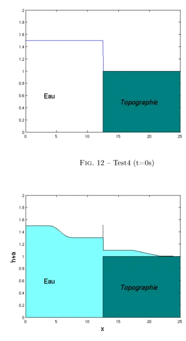
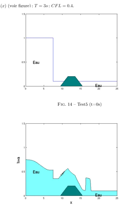
Figure


Documents relatifs
Keywords : Shallow water, mixed flows, free surface flows, pressurized flows, curvilinear transformation, asymptotic analysis, VFRoe scheme, well-balanced finite volume
The current R&D projects, NBVT, TTY, CCTV, and FAX, do not meet consumer needs on 'effectiveness' and 'ease of use' as well as the existing technologies of personal
Trace-element modeling can test further the potential link between trachydacite fiamme and rhyolitic composi- tions as, respectively, end-members of the leftover cumu- late and
Thanks to Theorem 5.2, we obtain a first order error estimate, in terms of the space step, for the hybrid 1D-2D finite volume scheme. This proves that the scheme is as accurate as
L’intérêt de notre étude était d’étudier l’incidence et les facteurs influençant sur la survenue de ces complications, qui sont loin d’être
Here we describe a strategy based on a local subsonic steady state reconstruction that allows one to derive a subsonic-well-balanced scheme, preserving exactly all the subsonic
Under a simple geometrical assumption for the clusters, we obtain that the pair of discrete spaces associating the classical cell-centered approximation for the velocities
The exploitation of the parallel processing power of GPU is interesting in comparison to a single-core GPU if the problem size of the finite volume solver for shallow water
