An energy-based variational model of ferromagnetic hysteresis for finite element computations

HAL Id: hal-01004989

https://hal.archives-ouvertes.fr/hal-01004989

Submitted on 6 Nov 2018

HAL is a multi-disciplinary open access

archive for the deposit and dissemination of

sci-entific research documents, whether they are

pub-lished or not. The documents may come from

teaching and research institutions in France or

abroad, or from public or private research centers.

L’archive ouverte pluridisciplinaire HAL, est

destinée au dépôt et à la diffusion de documents

scientifiques de niveau recherche, publiés ou non,

émanant des établissements d’enseignement et de

recherche français ou étrangers, des laboratoires

publics ou privés.

An energy-based variational model of ferromagnetic

hysteresis for finite element computations

V. François-Lavet, F. Henrotte, Laurent Stainier, Ludovic Noels, Christophe

Geuzaine

To cite this version:

V. François-Lavet, F. Henrotte, Laurent Stainier, Ludovic Noels, Christophe Geuzaine. An

energy-based variational model of ferromagnetic hysteresis for finite element computations. Journal of

Com-putational and Applied Mathematics, Elsevier, 2013, 246, pp.243-250. �10.1016/j.cam.2012.06.007�.

�hal-01004989�

An energy-based variational model of ferromagnetic hysteresis for finite

element computations

V. François-Lavet

a

_{, F. Henrotte}

b

_{, L. Stainier}

c

_{, L. Noels}

d

_{, C. Geuzaine}

a

a_{Université de Liège, Department of Electrical Engineering and Computer Science, Montefiore Institute B28, Grande Traverse 10, 4000 Liège, Belgium} b_{Université catholique de Louvain, iMMC, Bâtiment Euler, Avenue Georges Lemaître 4, 1348 Louvain-la-Neuve, Belgium}

c_{Ecole Centrale de Nantes, GeM, 1 rue de la Noë BP 92101 44321 Nantes cedex 3, France} d_{Université de Liège, LTAS-MCT B52, Chemin des chevreuils 1, 4000 Liège, Belgium}

Keywords: Magnetic hysteresis Variational formulations Finite element methods This paper proposes a macroscopic model for ferromagnetic hysteresis that is well-suited

for finite element implementation. The model is readily vectorial and relies on a consistent thermodynamic formulation. In particular, the stored magnetic energy and the dissipated energy are known at all times, and not solely after the completion of closed hysteresis loops as is usually the case. The obtained incremental formulation is variationally consistent, i.e., all internal variables follow from the minimization of a thermodynamic potential.

1. Introduction

Empirical models are essentially interpolated measurements. They offer a continuous representation of measurements, which are discrete by nature. Hysteresis models such as the Preisach or Jiles–Atherton models [1–3] belong to this category. The choice of their particular family of interpolation basis functions is based on their ability to accurately reproduce the measured data.

Because of their lacking a true thermodynamical background, empirical models suffer in general from poor accuracy when evaluated outside the ranges where measured data is available, hence the observed trend towards carrying out extensive and expensive measurement campaigns. In practice, however, it is impossible to calibrate a model for all possible conditions— even though an important role of a model is precisely to predict material responses in situations where measurements are difficult or impossible to obtain. In addition, most of the hysteresis models currently used in the electromagnetics community [1–4] are fundamentally scalar models. In order to generalize them to 2D or 3D they must be vectorized, an operation quite artificial and for which a true theoretical basis is lacking.

Some naturally vectorial approaches do exist: a first one is to treat the problem directly at the microscopic level and use multi-scale techniques [5,6] to trace the useful microscopic information over to the macroscopic level. The microscopic scale is that of Weiss domains and Bloch walls. These techniques are definitely relevant to improve the understanding of the microscopic phenomena involved. However, considering their very high computational cost, they are impracticable in modeling engineering applications. A second approach is based on the optimization of the parameters of parametric algebraic models so as to match measured hysteresis curves, e.g., via neural networks [7]. This approach gives interesting results, but as with all empirical models the connection with thermodynamics is lost and the energy consistency is not necessarily ensured.

The purpose of this paper is to go beyond the limitations of current models and to propose a vectorial hysteresis model with a clear-cut relation to the fundamental principles of thermodynamics, and therefore a wide applicability. We will show that the proposed model is numerically efficient and can be easily incorporated into existing Finite Element (FE) codes. 2. Thermodynamic foundation

2.1. Basic principles

In a ferromagnetic material, the first law of thermodynamics, stating conservation of energy, writes

˙

u

= ˙

W

+ ˙

Q

=

h

· ˙

b

−

div q

,

(1)

where u is the internal energy, W and Q are the amounts of work and heat supplied to the system, h and b are the magnetic field and the magnetic induction, and q is the heat flux. (The dot above a symbol stands for the time derivative.)

The second law of thermodynamics states that there exists a quantity s called entropy such that:

˙

s

≥ −

div

�

q

T

�

,

(2)

where T is the temperature and q

/T is the entropy flux. This equation can be rewritten as

T

˙

s

+

div q

−

q

·

grad T_T

≥

0

.

(3)

The first two terms in(3)define the dissipation functional

d

:=

Ts

˙

+

div q

,

(4)

whereas the third term corresponds to the thermal dissipation. Using(4), Eq.(1)becomes

˙

u

₊

d

₌

h

· ˙

b

+

T

˙

s. (5)

In a thermodynamic approach, functionals are primary quantities from which constitutive relationships are derived by application of general principles. The actual characteristics of the considered ferromagnetic material are thus introduced in the system by selecting appropriate expressions for the functionals u and d.

2.2. Ferromagnetic materials

The proposed model builds on the thermodynamic representation of the hysteresis proposed in [8–10], but additionally provides a complete variational setting inspired from the kinematic hardening theory of plasticity [11–13]. The first and second principles of thermodynamics are explicitly accounted for in the formulation of the model, which is based on the following simplifying assumptions that have proved to be largely correct in practice: (i) Hysteresis losses and eddy current losses can be decoupled, and hence treated separately in a model. This assumption has been discussed in detail in [1], and we thus only deal with hysteresis losses in this paper. (ii) The induction field

b

:=

J0

+

J (6)

is a sum of two components: an empty space magnetic polarization J0

:= µ

0h (where

µ

0is the magnetic permeability of vacuum), which is always linear and reversible, and a material magnetic polarization J, associated with the presence of microscopic moments attached to the atoms of the material body, and that can be both nonlinear and irreversible. (iii) Hysteresis losses can be interpreted as the power delivered by a constant amplitude generalized force parallel to the variation of the magnetic polarization, i.e., the magnetic equivalent of a dry friction force [9]. The physical origin of this force is the pinning effect that opposes the motion of Bloch walls.

Entropy is assumed constant in what follows (

˙

s

=

0), i.e., thermal effects are neglected. Moreover, in order to focus on the main aspect of the paper, which is the modeling of the hysteresis behavior, the terms involving the empty space magnetic polarization J0are provisionally disregarded until Section3.

2.3. Differential model

Under the assumptions detailed above, the energy density u is a function of J only and one has

u

=

u(J

),

u

˙

=

hr

· ˙

J

,

with hr

:= ∂

Ju. (7)

The dissipation function d describing magnetic hysteresis as a magnetic analogous of a dry friction force reads

d

= χ|˙

J

| =

hi

· ˙

J

,

with hi

:= ∂

˙Jd

= χ

˙

J

Fig. 1. Graphical representation of the vector equation(9). Left: simplest model with one internal variable (one sphere). Right: model with N=3 spheres.

Substituting(7)and(8)into(5)yields

(

h

−

hr

−

hi

)

· ˙

J

=

0. As the latter identity must always be true, the factor between

parentheses vanishes and the following governing equation for the ferromagnetic material is obtained:

h

−

hr

−

hi

=

0

,

or h

− ∂

Ju

− χ

˙

J

|˙

J

|

=

0

.

(9)

Since

χ

is a constant and

˙

J

/

|˙

J

|

is a unit vector, the vector equation(9)can be given the graphical representation given in Fig. 1(left). The vector hr is linked with the magnetic polarization of the material J by(7), and the tip of the applied field h

is located inside a sphere of radius

|

hi

| = χ

centered at the tip of hr. (A further interpretation when J is decomposed into

several parts will be given in Section2.6.)

2.4. Variational model

The governing equation(9) obtained in the previous section is a differential one. It can be discretized in time and implemented directly in a time-stepping FE model. This is for the most part the approach of Henrotte et al. in [9] where, however, a simplified case is presented: the unit vectorJ

˙

/

|˙

J

|

is assumed parallel to the vector h

−

hr

(

Jp

)

, where Jpis the value

of J at the previous time step, instead of parallel to h

−

hr

(

J

)

, where J is the value at the current time step. This simplification

makes the update algorithm explicit and avoids carrying out nonlinear iterations.

If one wants an exact solution of(9), a robust method to solve the nonlinear problem is required. An interesting approach consists in building a functional of J whose minimization at each time step amounts to solve(9). This variational approach is inspired from the kinematic hardening theory of plasticity [11]. The functional is determined in two steps.

First, the functional

g(h

,

J

)

:=

u(J

)

−

h

·

J (10)

is formed, such that

∂

Jg

= ∂

Ju

−

h

.

(11)

Second, one notes that d is a function of

˙

J (see(8)), whereas the sought functional should be a function of J. This is solved by defining a pseudo-potential D(J

,

Jp

)

:= χ|

J

−

Jp

|,

(12) whose gradient

∂

JD

= χ

J

−

Jp

|

J

−

Jp

|

≈ χ

˙

J

|˙

J

|

=

hi (13)

is a good approximation of the gradient of d for sufficiently small time steps. Eq.(9)can thus finally be rewritten as

∂

J

(g

+

D)

=

0

,

(14)

and the sought functional is

Ω

(

h

,

J

,

Jp

)

=

g

(

h

,

J

)

+

D(J

,

Jp

).

(15)

The updated value of J follows from minimizingΩat each time step. This variational update is a time-discretized variational

statement of the constitutive relation(9).

The constitutive behavior of the ferromagnetic material is thus completely determined by two quasi-thermodynamic functionals: the potential g, which is related to the magnetic energy u, and the pseudo-potential D. The equivalent of the yield surfaces of the kinematic hardening is, in the case of the ferromagnetic material, the sphere depicted inFig. 1(left).

There exists an analogy with the stress–strain model of St Venant with hardening. Hardening is introduced by connecting nonlinear springs in parallel with a slider, i.e., a friction element characterized by a limit force

χ

. The magnetic field h

Fig. 2. Pictorial representation of the model with N internal variables.

magnetic field h is increased. Before it reaches the limit

χ (

h

< χ )

, the applied field is equilibrated by the force of the slider,

and no polarization occurs (

˙

J

=

0). When h reaches the limit force

χ

, the slider is set into motion, which means that the

polarization J increases. The power delivered in the slider

χ ˙

J is dissipated, whereas the recoverable energy stored in the

spring increases. When the magnetic field h comes down below

χ

again, the slider gets locked, and polarization is frozen

(

˙

J

=

0).

2.5. Saturation characteristic

It is necessary to build the functional u to select a parametric saturation curve, whose parameters will be identified from measurements. In the case of nonoriented steels, it is enough to work with a simple scalar saturation curve like

hr

(x)

= α

atanh

(x/J

S

),

(16)

and to assume that the vector field hris parallel with J:

hr

(

x

)

=

hr

(

|

x

|)

x

|

x

|

.

(17)

The advantage of the atanh function is that it can be derived and integrated analytically. (Other choices could also be made: see e.g. [9].)

The saturation curve (16)depends on two parameters only: JS is the saturation magnetic polarization, and

α

is a

characteristic magnetic field inversely proportional to the slope of the curve at the origin. The corresponding expression for the magnetic energy is obtained by integration:

u(J)

:=

�

J 0 hr

(x)

dx

= α

JS

�

J JS atanh

�

_J JS

�

+

1₂ln

�

�

�

�

�

�

_J JS

�

2

−

1

�

�

�

�

�

�

.

(18)

2.6. The model with N spheres

The accuracy of the hysteresis model depends on the representation of the statistical distribution of the pinning point strengths in the material. The characteristics of this distribution vary largely across the different types of soft and hard ferromagnetic materials. This can be accounted for in the model by (i) dividing the magnetic polarization J into N parts

J

=

N

�

k=1

Jk ₍₁₉₎

and (ii) defining for each part Jk_{a time-independent pinning force}

_χ

k_{. This piecewise representation has practical advantages}

regarding the implementation and implies no limitation of the accuracy as the number of divisions N can be chosen arbitrarily large. (Higher order (non-piecewise) representations could be considered as well at the expense of a more sophisticated implementation.)

The Jk_{’s are the internal variables of the hysteresis model. Since they are additive (cf.(19)), they are all subjected to the}

same applied magnetic field h. The situation can be pictorially represented as the series connection of N cells (Fig. 2). The elongation of each cell corresponds to a partial polarization Jk_{, which is caused by the applied field h minus the force exerted}

by the parallel connected slider with threshold force

χ

k. The saturation law for each cell is hk

r

(x)

= α ·

atanh

(x/J

Sk

),

hkr

(

x

)

=

hkr

(

|

x

|)

_|

x_x

_|

,

(20)

and the total energy density is assumed to be simply the sum of cell-based energy densities:

u

:=

N

�

k=1 uk

₍

_Jk

_),

_uk

₍

_Jk

₎

_:=

�

J k 0 h k r

(x)

dx

= α

JSk

�

Jk Jk S atanh

�

_Jk Jk S

�

+

1₂ln

�

�

�

�

�

�

_Jk Jk S

�

2

−

1

�

�

�

�

�

�

.

(21)

Table 1

Identified parameters for electrical steel M250-50A with 3 internal variables (a) and 5 internal variables (b).

k JS[T] χ_[A/_m] (a) 0 0.11 0 1 0.8 16 2 0.31 47 (b) 0 0.11 0 1 0.3 10 2 0.44 20 3 0.33 40 4 0.04 60

Fig. 3. Accuracy of the model as a function of the number of internal variables. As the dissipation functional reads

D

=

N

�

k=1

χ

k

|

Jk

−

J_pk

|,

(22)

the functionalΩ(15)can be written as a sum of independent cell-basedΩkfunctionals

Ω

=

N

�

k=1 Ωk

(

h

,

Jk

,

J_pk

)

=

N

�

k=1

�

_uk

₍

_Jk

₎

₋

_h

_·

_Jk

_{+ χ}

k

_|

_Jk

₋

_Jk p

|

�

(23)

that can be minimized separately. Knowing h at the current time step, and Jk

p at the previous time step in each cell, the

minimization ofΩkdelivers the updated value of Jkat the current time step. The magnetic field h and the yield surfaces in

a model with three spheres are depicted inFig. 1(right). 3. Application

3.1. Parameter identification

Working with N cells, the hysteresis model has 2N

+

1 parameters to identify: the initial saturation slope

α

, which is

identical for all cells (this is an empirical result) and the 2N cell-specific parameters Jk

S and

χ

k. A standard non-oriented

electrical steel grade M250-50A [14] has been used in this paper to test the new model. The identification can be done easily on basis of the first magnetization curve (virgin curve) of the material, measured with e.g. an Epstein frame or a Single Sheet Tester. By comparing the modeled first magnetization curve with the measured one for increasing values of the applied field

h, the pairs

(J

k

S

, χ

k

)

can be identified systematically for increasing values of

χ

k. The identified parameters are

α

=

65

[

A/m

]

,

and those given inTable 1for a hysteresis model with 3 and 5 internal variables, respectively.

Fig. 3shows the accuracy of the model as a function of the number N of internal variables. A rapid decay of the error is observed as the number of internal variables increases. Reasonably accurate models are thus obtained with relatively few parameters.

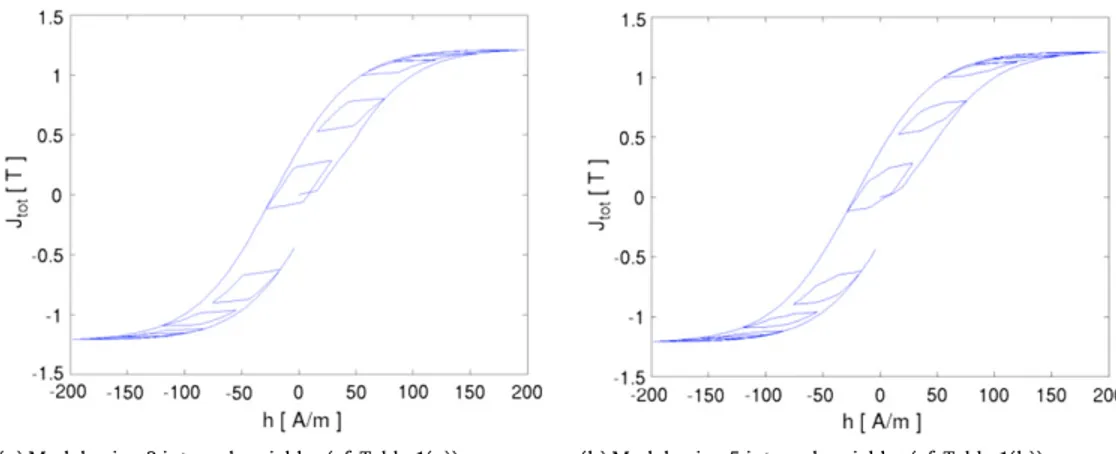
(a) Model using 3 internal variables (cf.Table 1(a)). (b) Model using 5 internal variables (cf.Table 1(b)).

Fig. 4. Main and minor hysteresis loops of M250-50A steel modeled with 3 or 5 internal variables, when a 10-th harmonic is superimposed to the main

frequency.

Fig. 5. Total magnetic losses associated with the M250-50A hysteresis cycle when increasing the amplitude of the 10-th harmonic superimposed to the

main frequency.

3.2. Minor loops and higher harmonics

The hysteresis model proposed in this paper represents a significant improvement with respect to conventional post-processing techniques based on measured loss characteristics. Because it relies on a physical assumption that it is vectorial and dynamic from the beginning (the analogy with a dry friction force), the identified parameters represent the material in general, and not under specific experimental conditions. In other words, although the identification was done with experimental data assuming a sinusoidal in time and unidirectional b field, the identified parameters given inTable 1can be used in 2D and 3D, and in the presence of higher harmonics.Fig. 4shows the main and minor loops obtained with resp. 3 and 5 internal variables when the applied field h consists of a fundamental harmonic with a 10th higher harmonic superposed. The general aspect of the hysteresis loops is already good with 3 internal variables, but the shape of the minor loops is more realistic with 5 internal variables. This is confirmed by analyzing the computed losses.

Fig. 5shows a comparison between the hysteresis losses calculated by integration over time of the value of the dissipation functional(22)with 3, 5 and 8 internal variables. It is observed that the gain of accuracy between 5 and 8 internal variables is already much less significant than the one between 3 and 5 internal variables. Once again, it may be concluded that a relatively small number of internal variables is sufficient to obtain an accurate representation of the complex response of the material.

3.3. Finite element implementation

The ferromagnetic material relationship is

h

=

b

−

�

N

k=1J

k

and we shall work with the magnetic vector potential a (with b

=

curl a), so that Gauss’ law div b

=

0 is automatically satisfied. The weak formulation of Ampere’s law then reads [15,16]: Find a such that

�

Ω 1

µ

0curl a

·

curl a �_dΩ

₋

�

N k=1

�

Ω 1

µ

0J k

_·

_{curl a}�_dΩ

₌

�

Ω js

·

a�dΩ (25)

holds for a set of suitably chosen test functions a�_{(jsbeing a given source current density). These finite element equations} are nonlinear because the N internal variables Jk_{are the result, in each element, of the implicit relationship}

Jk

₌

_Update

₍

_h

_,

_Jk p

),

with h

=

curl a

−

�

N k=1J k

µ

0

.

(26)

The detailed algorithm is as follows: Algorithm 1: Finite Element Algorithm 1 Initialize J_pk

=

0;

2 for t

=

1

:

tmaxdo

// Time loop

3 while∆a

<

criterion do

// Picard iteration

4 for all finite elements do

// Assembly loop

5 Update internal variables Jkusing (26); 6 Assemble element in the linear system (25); 7 Solve linear system;

A Picard iteration loop is done at each time step to resolve the nonlinearity. In each iteration of the Picard scheme, the ‘‘Update’’ function in(26)minimizesΩk(23). Amongst the many robust optimization schemes available, a first-order

descent method has been chosen in our implementation. Since the functionalΩkhas an angular point when h_i

�=

0, which

might impede convergence, the descent algorithm uses J

=

Jpas an initial guess. In our tests this makes the minimization

algorithm always converge in less than 20 iterations. Overall, the hysteresis model requires the storage of 2N additional vector unknowns (Jk_{and J}k

p) per element.

As an application example, a three-phase transformer has been analyzed. The material data ofTable 1(a) has been used to model the ferromagnetic behavior of the core of the transformer.Fig. 6shows a closeup on the central T-joint of the core, i.e., on the region where the fields are not unidirectional. The trajectory of the tips of the b (solid line) and the h (dotted line) vectors are represented at 4 selected points over about one period. Clearly, the main aspects of the ferromagnetic behavior, namely the vector character, saturation and the lagging behind of b with respect to h, are correctly represented by the model. 4. Conclusion

The motivation for this work is the development of constitutive models for hysteresis phenomena. The proposed model, based on thermodynamic principles, is energy-consistent. A variational approach provides a robust and coherent framework to efficiently handle the strong nonlinearity of the problem within a finite element scheme. The use of a dissipation functional and its connection with yield surfaces was inspired by modern approaches of kinematic hardening. Besides mathematical and physical elegance, this model has practical advantages. Unlike the model of Preisach and Jiles–Atherton, it is readily vectorial and the number of parameters is not limited. Moreover, it relies on an energy balance, of which the stored magnetic energy and dissipated energy are known at all times.

With this approach, hysteresis losses, accounting for vector effects (rotating hysteresis) and the presence of higher harmonics, can be evaluated with controllable accuracy. This opens up the possibility of accurate evaluations of magnetic losses in real-life electrical engineering devices: from the prediction of iron losses in electrical engineering devices (rotating machines, actuators, brakes) to the accurate modeling of hysteresis in magnetostrictive actuators and smart materials.

Quantitative loss comparisons and a more systematic parameter identification methodology are currently under investigation. Another further improvement will be to deal with laminated structures explicitly by means of appropriate multi-scale techniques. Finally, we have only considered the special case of rate-independent isotropic materials. Further developments to handle rate effects and anisotropy would clearly be of interest.

Acknowledgments

This work was supported in part by the Belgian Science Policy (IAP P6/21), Belgian French Community (ARC 09/14-02) and Walloon Region (WIST3 No 1017086 ‘‘ONELAB’’).

Fig. 6. Magnetic and induction field in the central T-joint of a three-phase transformer over about one period. The dotted line is the h-field and the solid

line is the b-field obtained with three internal variables Jk_{(cf.Table 1(a)).} References

[1] G. Bertotti, Hysteresis in Magnetism, Academic Press, 1998.

[2] I. Mayergoyz, Mathematical Models of Hysteresis and their Applications: Second Edition, Academic Press, 2003.

[3] D.C. Jiles, D.L. Atherton, Theory of ferromagnetic hysteresis, Journal of Magnetism and Magnetic Materials (1986) North-Holland, Amsterdam. [4] A. Benabou, S. Clenet, F. Piriou, Comparison of Preisach and Jiles–Atherton models to take into account hysteresis phenomenon for finite element

analysis, Journal of Magnetism and Magnetic Materials (2003).

[5] Ben van de Wiele, et al., Energy considerations in a micromagnetic hysteresis model and the Preisach model, Journal of Applied Physics 108 (2010) 103902.http://dx.doi.org/10.1063/1.3505779.

[6] G. Bertotti, Connection between microstructure and magnetic properties of soft magnetic materials, Journal of Magnetism and Magnetic Materials 320 (2008) 2436–2442.

[7] T. Matsuo, M. Shimasaki, Two types of isotropic vector play models and their rotational hysteresis losses, IEEE Transactions on Magnetics 44 (6) (2008) 898–901.

[8] A. Bergqvist, Magnetic vector hysteresis model with dry friction-like pinning, Physica B 233 (1997).

[9] F. Henrotte, A. Nicolet, K. Hameyer, An energy-based vector hysteresis model for ferromagnetic model, Selected Papers from the EPNC’2004 Symp., Poznan, Poland, June 28–30, 2004.

[10] F. Henrotte, K. Hameyer, A dynamical vector hysteresis based on an energy approach, IEEE Transactions on Magnetics 42 (4) (2006).

[11] A.M. Puzrin, G.T. Houlsby, Fundamentals of kinematic hardening hyperplasticity, International Journal of Solids and Structures 38 (2001) 3771–3794. [12] A.M. Puzrin, G.T. Houlsby, A thermomechanical framework for constitutive models for rate-independent dissipative materials, International Journal

of Plasticity 16 (2001) 1017–1047.

[13] M. Ortiz, L. Stainier, The variational formulation of viscoplastic constitutive updates, Computer Methods in Applied Mechanics and Engineering 171 (1999) 419–444.

[14] ThyssenKrupp, Publications/Product Information/Electrical Steel No: www.thyssenkrupp-steel-europe.com/tiny/Cp/download.pdf (accessed 05.09.11).

[15] N. Ida, J.P.A. Bastos, Electromagnetics and Calculation of Fields, Springer, 1992.

[16] P. Dular, C. Geuzaine, F. Henrotte, W. Legros, A general environment for the treatment of discrete problems and its application to the finite element method, IEEE Transactions on Magnetics 34 (5) (1998) 3395–3398.