CIRPÉE
Centre interuniversitaire sur le risque, les politiques économiques et l’emploi
Cahier de recherche/Working Paper 06-33
Rules of Proof, Courts, and Incentives
Dominique Demougin Claude Fluet
Octobre/October 2006
_______________________
Demougin: Humboldt Universität zu Berlin and CIRPÉE [email protected]
Fluet: Université du Québec à Montréal and CIRPÉE [email protected]
Preliminary versions of this paper were presented at the Workshop on Law and Economics, Stony Brook Game Theory Festival, July 2005, and at the EALE Annual Conference, Madrid, September 2006. We thank Andrew Daugherty, Chris Sanchirico, Steve Mongrain, Hans-Bernd Schäfer, Kathryn Spier, Eric Talley and Joel Watson for helpful comments. Financing from FQRSC (Quebec) and SSHRC (Canada) is gratefully acknowledged.
Abstract:
We analyze the design of legal principles and procedures for court decision-making in civil litigation. The objective is the provision of appropriate incentives for potential tort-feasors to exert care, when evidence about care is imperfect and may be distorted by the parties. Efficiency is shown to be consistent with courts adjudicating on the basis of the preponderance of evidence standard of proof together with common law exclusionary rules. Inefficient equilibria may nevertheless also arise under these rules. Directing courts as to the assignment of the burden of proof is then useful as a coordination device. Alternatively, burden of proof guidelines are unnecessary if courts are allowed a more active or inquisitorial role, by contrast with that of passive adjudicator.
Keywords: Evidentiary rules, standard of proof, burden of proof, inquisitorial,
adversarial, discovery, deterrence
1
Introduction
Court decision-making is constrained by various rules and standards. In common law, exclusionary rules discard as inadmissible apparently relevant evidence. This includes evidence of similar facts (e.g., whether the defen-dant was previously involved in a similar case), evidence of character or of a reputation for behaving negligently or diligently, or evidence purporting to show that defendants of a particular type tend to behave in a particular way. In civil litigation, courts must decide on the basis of a preponderance of evidence, a standard of proof requirement. The preponderance standard means that a claim is deemed proved if, upon the evidence, it is more likely true than not true. There are also situations where the law imposes on courts the burden of proof assignment. For instance, rather than having the plain-ti¤ bear the burden as is usually the case, statute law or jurisprudence may require that the defendant prove that he did not cause harm or did not act negligently. In some cases, burden of proof requirements may also refer to the type of evidence needed for proof. Finally, there are legal traditions where the court is allowed a more active or inquisitorial role, by contrast with that of passive adjudicator in the purely adversarial procedure of common law. We develop a model of tort litigation where the above legal principles and procedures can be analyzed on e¢ ciency grounds.
To illustrate, consider a medical liability case. The plainti¤ claims that he su¤ered harm due to negligent oversight by his physician. Suppose all relevant evidence always becomes available to the court. The evidence may nevertheless be highly imperfect, i.e., the court faces a risk of error whether it rules in favor of the patient or the physician. An important issue is therefore the “degree of certainty” or standard of proof required to reach a decision. Demougin and Fluet (2006) show that the preponderance standard has a remarkable property. If courts rule on the issue of negligence on a prepon-derance of evidence, there will be maximum ex ante incentives for physicians to act nonnegligently. The argument has a caveat: in applying the stan-dard, courts must abide by exclusionary rules. Evidence pertaining to a
“propensity” for the defendant to act a certain way should be discarded as inadmissible. There is therefore an e¢ ciency justi…cation for the standard of proof and exclusionary rules in common law.1
The above result was derived under the assumption that evidence exoge-nously becomes available to the court. This paper extends the analysis to the case where veri…able evidence initially rests with the parties, who may attempt to shade the evidence. This introduces additional di¢ culties such as the weight that should be given to a testimony or the appropriate inter-pretation of the evidence submitted. If evidence can be manipulated, is a preponderance of evidence still the appropriate standard? And what does a preponderance mean?
The issue is straightforward if both litigants are known to have access to all veri…able evidence and if submission costs are small compared to the stakes. As evidence will necessarily favor one party or the other, one of the “interested party”will …nd it useful to disclose it (Milgrom and Roberts, 1986). Equivalently, if all relevant evidence is not disclosed, a Bayesian judge or jury will draw the appropriate inferences. However, unraveling does not follow if the parties do not always have access to all the evidence and may be unequally informed. Shavell (1989) and Shin (1994, 1998) showed that the parties may then be successful in not revealing facts harmful to their case.
The court’s problem is then to interpret partial and possibly distorted information. Should this a¤ect the standard of proof and exclusionary rules described above? If plainti¤s in medical liability cases are known to be able on average to present only basic evidence, should the standard of proof they must meet be lower? Should some weight now be given to the physicians’general propensity to act negligently? We show that, even though the parties can manipulate the submitted evidence and may be unequally informed, courts should abide by exactly the same rules of proof as above.
We assume that, in applying these rules, courts are sophisticated
decision-1Schrag and Scotchmer (1994) analyzed the deterrence justi…cation for the dismissal of
makers, i.e., they understand the parties’ strategic incentives. As a result, they interpret limited evidence in a particular light. Suppose the plainti¤ submits “mixed” evidence. By this we mean evidence which, under the preponderance standard, is consistent with either a decision for the plainti¤ or against him, should additional evidence be forthcoming. Then it may be that, if the defendant does not come forward with countervailing evidence, the court will form a presumption against him. Such presumptions arise spontaneously, so to speak, in the manner courts interpret evidence under the preponderance standard.
So far, the implication seems to be that standard of proof and exclusionary rules are the only judicial tools needed to e¢ ciently direct court decision-making, i.e., these principles are su¢ cient if the objective of tort law is to provide potential tort-feasors with the best ex ante incentives to exert care. There is nevertheless a sense in which the foregoing result does not necessarily follow. While an e¢ cient equilibrium exists when courts operate under the appropriate standard of proof and exclusionary rules, other equilibria may exist as well under the same set of rules.
To see this, suppose again the victim most likely has access to only limited evidence. Assume that e¢ ciency requires that the defendant be held liable given this evidence on its own. If in equilibrium the court holds a presumption against the defendant when this evidence is the only one submitted, then the victim will sue on the basis of this evidence alone. Moreover, the court will be justi…ed, under the preponderance standard, to …nd that there was negligence. The reason is that, owing to the presumption against him, the defendant would most likely have come forward with additional evidence if it was in his favor. The fact that he did not therefore justi…es the presumption. Call this equilibrium A, which by assumption here is the e¢ cient one.
Now, consider another possibility. In equilibrium B, the court does not …nd the defendant liable under the limited evidence alone. Hence, the victim does not sue on this basis alone. If he did, the defendant would have no incentive to come forward with additional costly evidence since he (correctly)
expects the plainti¤ to fail. Thus, the court will interpret the limited evidence di¤erently than in equilibrium A, because the defendant’s strategic incentives are di¤erent. As a result, the court concludes that the plainti¤’s evidence does not meet the standard of proof, i.e., that negligence has not been shown to be more likely than due care.
In circumstances such as these, imposing on courts the burden of proof assignment helps select the better equilibrium. In the example, courts should be directed to put the burden of proof on the defendant. The purpose is to co-ordinate parties and courts on the good equilibrium, making sure that victims come forward even if it they have limited evidence. Such guidelines— e.g., through statute law or jurisprudence from higher courts— are often observed. Although we formulated the example in terms of the need to put the burden of proof on the defendant, the reverse problem can also arise where courts are too lenient with plainti¤s.2
Burden of proof guidelines apply to large classes of cases, irrespective of the detailed information only available at the court level. Hence, guidelines will not always ensure coordination on the e¢ cient equilibrium. This leads us to inquire whether a modi…ed court procedure can eliminate the need for guidelines. Up to now, our stylized court involved a purely “passive” adjudicator whose only role is to decide at the close of the proceedings. The modi…ed procedure, as in the more “inquisitorial”trials of civil law countries, allows the adjudicator to intervene during the proceedings by interrogating the parties directly and purposely shifting the burden of proof. Speci…cally, the adjudicator announces how he will rule should no additional evidence be forthcoming (both binding and non binding announcements are considered). We show that the optimal liability assignment then obtains as the unique equilibrium if the active adjudicator abides by the preponderance standard and common law exclusionary rules. The interpretation is that, with a more
2In our analysis as in actual practice, the plainti¤ always bears the so-called “primary
burden”. Since he initiates the suit, he must provide some appropriate, albeit limited evidence if he is to stand a chance of winning.
active court, these rules of proof then su¢ ce for an e¢ cient “decentralization” of decisions regarding liability.
The paper develops as follows. Section 2 describes the basic tort situation that we have in mind. The next two sections assume that society can commit to a liability assignment as a function of the disclosed evidence, without yet introducing courts as ex post decision-makers. Section 3 analyzes the opti-mal scheme for the purpose of inducing care, i.e., we determine how liability should be assigned on the basis of the evidence made available by the par-ties. The liability assignment takes into account the potential tort-feasors’ex ante incentives to exert care and the parties’ex post incentives to submit and manipulate evidence. We show that the optimal scheme satis…es a “more-likely-than-not”property. Section 4 discusses how the mechanism can also be interpreted in terms of the allocation of the burden of proof. Section 5, which contains the main results, examines whether the optimal liability assignment can be obtained as an equilibrium when decisions regarding liability are del-egated to a court, now an additional player in the game. This requires that we analyze what general legal rules should constrain court decision-making. We show that the appropriate rules include the preponderance of evidence standard of proof and exclusionary rules as in common law. We discuss the need for burden of proof assignments as coordination device and the role of more inquisitorial courts. Section 6 reviews the related literature, discusses extensions, and concludes. Proofs are in the appendix unless statements are obvious from the text.
2
The Model
A party, denoted D, undertakes a socially valuable activity which may im-pose harm on a third party, denoted P , depending on how the activity is undertaken. If D exerts high care h, no harm is imposed. If low care l is taken, P su¤ers a loss of amount L. With low care D obtains a private bene…t c, for instance the cost savings from not exerting high care. When
c < L, low care is socially undesirable. The cost c is distributed according to the cumulative distribution function G(c), but it is privately known to D at each instance where a choice of care level must be made. Thus, if D were fully liable whenever he causes harm, he would exert high care in all instances where c < L, hence with probability G(L), which would be socially optimal.
The occurrence of harm, equivalently whether D undertook action l, is not directly veri…able. Only some body of evidence, denoted by x, is avail-able. This may include witness testimony about D’s behavior, expert opinion about whether P su¤ered harm, documents, etc. Ex ante, the content of the evidence x is uncertain with potential realizations in a countable set X and a probability distribution that depends on D’s care level. We denote this probability by pj(x), where j is either h or l, so that
P
x2Xpj(x) = 1. In this
formulation, it is possible that some realizations of the evidence reveal D’s behavior or the occurrence of harm perfectly. This occurs when ph(x) = 0
and pl(x) = 1 or conversely when ph(x) = 1 and pl(x) = 0. If this were true
for all x 2 X, the evidence would be fully informative. We assume this is not the case.3
To illustrate, suppose P has utility function u = ln q+w where w is wealth and q is an index of physical well-being, say the individual’s health status. If the physician or hospital takes high care, the potential health status is the random variableeqh while with low care it is eql = eqh, where < 1. In money
equivalents, the loss due to low care is L = ln . If the only evidence were the individual’s health status, i.e., x = q, this would generally constitute relatively poor evidence about the physician’s care, depending on the extent to which the supports of qeh and eql overlap. However, x could also include
additional direct evidence about the physician’s actions.
Party P (now the plainti¤) can sue party D (now the defendant) but can hope to prevail only by submitting evidence. We …rst consider the case
3We assume p
h(x) + pl(x) > 0 for all x 2 X (i.e., X is the union of the supports of the
where the parties have perfect access to the evidence x, assuming that the cost of submitting evidence is negligible. The issue is how liability should be assigned, on the basis of the evidence, in order to induce D to exert opti-mal care as often as possible. We impose the constraint that the defendant cannot be held liable for more than the possible loss (we discuss below the e¤ect of allowing “punitive damages”). Let (x) 2 [0; 1] denote the liability assignment. (x) = 1 means that the defendant is held liable for the full amount L when the evidence is x, (x) = 0 that he is not liable, while a value between zero and unity amounts to randomization or to damages for only a fraction of the potential harm.
For a given liability assignment function, D’s expected liability costs are LX
x2X
pj(x) (x); j = h; l:
Taking the cost c into account, D therefore chooses not to impose harm if X
x2X
[pl(x) ph(x)] (x)
c
L: (1)
The expression on the left-hand side, which we refer to as deterrence, is the increase in the probability of being held liable when action l is chosen rather than h.
It is easily seen that 1 under any , a value of unity being feasible only if the evidence perfectly reveals D’s behavior. With imperfectly infor-mative evidence, high care is exerted only when c L < L, which means that there is insu¢ cient deterrence. The best liability assignment function is therefore the one which maximizes deterrence— equivalently, which maxi-mizes the probability G( L) that no harm is caused.
Proposition 1 The deterrence maximizing liability assignment, as a func-tion of the evidence x 2 X, is (x) = 1 when pl(x) > ph(x), (x) = 0
otherwise.
To maximize deterrence, (x) should be set at its maximum value of unity when the expression in brackets in (1) is positive, and at its minimum
value of zero when the expression is negative. When the expression is nil, the value of (x) is indi¤erent. We set it equal to zero in this case, which may be interpreted as putting the burden of persuasion on the plainti¤.4
The proposition has a straightforward interpretation. pj(x) is the
prob-ability of the “data” represented by x conditionally on the hypothesis j 2 fh; lg being true. In statistical terminology, it would be referred to as the “likelihood” of hypothesis j on the basis of the observable data. Thus, the proposition states that the defendant should be liable when l is more likely than h, given the evidence. Under such a scheme and given a small cost of submitting evidence, when pl(x) > ph(x) the plainti¤ …les suit and submits
x, otherwise he does not …le suit.
Consider now the possibility of punitive damages B > L. A su¢ ciently large B can obviously implement the …rst best provided we do not run into bankruptcy problems. The potential defendant now exerts high care if
c BX
x2X
[pl(x) ph(x)] (x):
Optimal care requires that B be set so that L = BX
x2X
[pl(x) ph(x)] (x):
This can be satis…ed in an in…nite number of ways, but clearly leads to the smallest level of punitive damages, say B , consistent with the …rst best. Thus, another justi…cation for the liability assignment function of proposition 1 is that it minimizes the punitive damages consistent with inducing optimal care.5 Alternatively, it may be that the defendant’s wealth is smaller than B , so that the …rst-best is unattainable. Holding the defendant liable up to
4The result is borrowed from Demougin and Fluet (2006)— see also Lando (2002) for a
similar …nding. Note that society is asumed to be indi¤erent to error per se. If error were socially costly, should take into account the trade-o¤ between deterrence and avoiding error (see Demougin and Fluet, 2005).
5Large punitive damages generate other distorsions since they in‡ate the cost of
his entire wealth and using is then the best one can do. In what follows, we stick to our earlier interpretation and assume compensatory damages, i.e., a liable defendant pays the plainti¤ the amount L.
We henceforth relax the assumption that the parties have perfect access to all the potential evidence. To discard straightforward unraveling results, we also assume that society, as Principal, does not know the extent of the veri…able evidence available to the parties. To make things as simple as possible, suppose the complete body of evidence can be partitioned as x = (y; z) with y 2 Y and z 2 Z(y) de…ned as the set of potential additional evidence consistent with the partial evidence y. Both parties always have access to y, but may not be able to also submit z. For example, the potential evidence could consist of the content of two separate “…les”. The parties always have access to the …rst …le y but may not be able to access the second …le z. Moreover, the parties may di¤er in their capacity to present veri…able evidence. Party P has access to z only with probability v, party D only with probability u, where u; v 2 (0; 1).
Any reasonable liability assignment scheme requires that P submit at least y in order to prevail. Indeed, P is the only party with an interest in initiating proceedings and it is known that part y of the evidence is accessible to him. However, as parties may be only partly informed, when only y is disclosed society does not know whether this is because the parties did not observe all the potential evidence or whether an informed party chose not to disclose z. We denote by the case where society does not receive the additional evidence. Note that we make the usual assumption that false evidence cannot be fabricated.
The issue is now to choose a liability assignment scheme of the form (y; z)2 [0; 1] where y 2 Y , z 2 Z(y) [ f g. Although the objective remains that of providing the best ex ante incentives to exert care— i.e., maximize deterrence— account must now be taken of the fact that will also a¤ect the parties’ ex post incentives to disclose evidence. In turn, this will have repercussions on D’s ex ante incentives to exert care.
3
Optimal Liability Assignment
The set-up is described by the following time line. First, society chooses at the outset a function for assigning liability, should P …le suit (no dam-ages are paid if no suit is …led). Second, Nature chooses c according to the distribution G(c), D observes c and decides between action h or l. Third, Nature chooses the evidence x = (y; z) according to the joint probability distribution pj(y; z) depending on whether j is h or l, where y 2 Y and
z 2 Z(y). Fourth, P (respectively D) observes z with probability v (re-spectively u); neither party knows whether the other has seen the complete potential evidence.
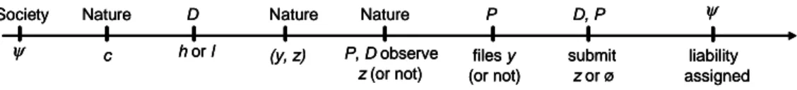
At this point, party P decides whether to …le suit, where …ling suit entails the submission of y. We call this the …ling stage. Next, if a suit has been …led, both parties decide simultaneously whether to submit additional evidence (if they can). We call this the disclosure stage. Finally, society assigns liability according to on the basis of the overall evidence submitted, (y; z) or (y; ) as the case may be. Notice that we do not yet discuss courts, but merely seek to characterize the deterrence maximizing liability assignment.6 Figure 1 summarizes the time line.
c Nature h or l D Nature (y, z) Nature P, D observe z (or not) files y (or not) P D, P submit z or ø Society ψ liability assigned ψ c Nature c Nature h or l D h or l D Nature (y, z) Nature (y, z) Nature P, D observe z (or not) Nature P, D observe z (or not) files y (or not) P files y (or not) P D, P submit z or ø D, P submit z or ø Society ψ Society ψ liability assigned ψ liability assigned ψ
Figure 1: Liability assignment function
Solving the game backwards, we …rst analyze the stages consisting of the decision to …le suit and the ensuing disclosure game. As before, submitting evidence is assumed to involve an arbitrarily small cost (we further discuss the role of submission costs at the end of the section). Such a cost is incurred by P if he …les suit and submits y. A similar cost is also incurred by any party submitting the additional evidence z. It is easily seen that the parties then
6 has the same interpretation as the “sanctioning function” in Shavell (1989), except
have dominant strategies. For instance, suppose the victim …led suit and the injurer observed z. If (y; z) < (y; ) the injurer discloses z since by doing so he reduces the probability of paying damages. If (y; z) (y; ) he does not reveal z. Note that a party’s belief as to whether the other party has observed z is irrelevant; the same is true of the victim’s belief about the defendant’s care level.7
Lemma 1 The following strategy pair is the unique equilibrium of the …le and disclosure game. (i) If P observes z and (y; ) < (y; z), P …les suit and discloses z at the next stage; if z is not observed or if (y; z) (y; ), P …les suit provided (y; ) > 0 but submits nothing at the next stage; in all other cases P does not …le suit. (ii) If a suit has been …led and (y; z) < (y; ), D discloses z if he can; otherwise he discloses nothing.
We denote by pj(y) the marginal probability of partial evidence y, given
that D has chosen action j. We write pj(zj y) for the conditional probability
of the additional evidence z 2 Z(y), given that the partial evidence is y and that care was j.
Conditional on y, the probability of D being held liable, when care level j was exerted, is equal to
ej(y) := (y; ) + v
X
z2Z(y)
pj(zj y) max[0; (y; z) (y; )]
u X
z2Z(y)
pj(zj y) max[0; (y; ) (y; z)]: (2)
The expression follows directly from the outcome of the disclosure game, tak-ing into account each parties’probability of accesstak-ing the complete evidence
7Bull and Watson (2004) develop a model where “veri…ability” is associated with the
enforcer’s actual observation of hard evidence. Taking y as given, think of each realization z 2 Z(y) as a particular “document”. The random draws with probability u or v determine whether D or P possesses the document. The document z is veri…able by the enforcer (i.e., will actually be observed by him) if D has the document and (y; z) > (y; ) or if P has it and (y; z) < (y; ).
and the incentives to disclose (the derivation is in the proof of proposition 2). Ex ante, as a function of the level of care, the probability of being held liable is therefore Py2Y pj(y)ej(y).
As in section 2, the best scheme is the one which maximizes the di¤erence in the probability of being held liable when low rather than high care is exerted. This means that must be chosen so as to maximize deterrence, now written as
=X
y2Y
[pl(y)el(y) ph(y)eh(y)]: (3)
Proposition 2 When the parties may be only partly informed, deterrence is maximized by (y; z) as de…ned in proposition 1 when z 2 Z(y), (y; ) = 1 if pl(y)Ql(y) > ph(y)Qh(y) and (y; ) = 0 otherwise, where
Qj(y) (1 v)(1 u) + (1 u)v X z2Z(y) [1 (y; z)] pj(z j y) + (1 v)u X z2Z(y) (y; z) pj(z j y); j = h; l: (4)
The expression in (4) is the conditional probability of z not being revealed given D’s care level and the realization y. The rationale is that z remains undisclosed either because both parties are uninformed or only one is in-formed but would not disclose evidence unfavorable to his case. pj(y)Qj(y)
is therefore the probability of the event “partial evidence is y and z not revealed” given D’s ex ante action. Recalling statistical terminology once more, the expression is the likelihood of action j on the basis of the available “data”. Thus, the proposition shows that the more-likely-than-not property still holds even when disclosure is an issue. However, the probability as-sessments now take into consideration the parties’ capability of submitting evidence and their motive for not disclosing.8 Notice that 2 f0; 1g as in the previous section, i.e., the liability assignment is all-or-nothing.
8The result is derived for a binary partition of the body of evidence, but the argument
Small submission costs ensured a unique equilibrium in the …le and dis-closure game. However, the non uniqueness that would arise with zero costs is inconsequential, i.e., is also deterrence maximizing if submission costs are nil. For instance, when (y; z) = (y; ), an informed defendant would be indi¤erent between disclosing and not disclosing. Whether he does or not, the liability assignment and therefore deterrence remain the same.
A more interesting extension is when the cost of submitting z is non neg-ligible. Recalling that is all-or-nothing, the disclosure strategies described in lemma 1 remain dominant strategies as long as the cost of submitting z is smaller than the stakes represented by L. It follows that is still deter-rence maximizing. We henceforth continue to assume that the cost of …ling suit and submitting y is small, but allow that of submitting z to be non negligible.9 The interpretation is that y concerns the basic facts of the case
and is straightforward to submit, while z involves more complex evidence. Although submission costs play no role at this stage, they will be relevant when we discuss court decision-making.
4
Burden of Proof
In legal terminology, the plainti¤ is said to bear the burden of proof if he loses unless he produces enough evidence supporting his claim. Conversely, the burden rests on the defendant if he is held liable unless he produces evidence in his favor. The procedure is nevertheless always initiated by the plainti¤ who bears the “primary burden” of establishing that the case is worth hearing. In the model, this is captured by the fact that the plainti¤ must …le suit in order to obtain damages and cannot but submit y when a suit is …led. In what follows, the burden of proof (or so-called “burden of production”) refers to how the task of producing the additional evidence is
9However, we assume it is not too large, otherwise it could be relevant for society to
consider the trade-o¤ between deterrence and litigation costs, an issue we wish to avoid at this point. We discuss it in the conclusion.
apportioned between the parties.
Given the partial evidence y, the scheme assigns the burden to the plainti¤ if (y; ) = 0 and to the defendant if (y; ) = 1. There is a quali…cation. It may be that none of the parties has an incentive to submit additional evidence because (y; z) = (y; ) for all z 2 Z(y). This occurs when z is insu¢ ciently informative compared to y. We say that y constitutes mixed evidence if there exists z, z0 2 Z(y) such that p
l(y; z) > ph(y; z) and
pl(y; z0) ph(y; z0), implying that the liability assignment can go either way
depending on what additional evidence is submitted. Otherwise, y represents conclusive evidence.10
When y is conclusive, either pl(y; z) > ph(y; z)for all z 2 Z(y), yielding
pl(y) > ph(y), or pl(y; z) ph(y; z) for all z 2 Z(y), yielding pl(y) ph(y).
Moreover, Qh(y) = Ql(y) as is easily seen from (4). Disclosing additional
evidence then cannot change the liability assignment. By contrast, when y is mixed, one of the parties bene…ts from disclosing additional evidence in his favor. Thus, (y; ) captures the concept of burden of proof only when the partial evidence is mixed. The next results characterize the optimal liability assignment.
Corollary 1 If y is conclusive or if u = v, (y; ) = 1 if pl(y) > ph(y), otherwise (y; ) = 0.
When the partial evidence is conclusive, disclosing additional evidence is irrelevant. Liability is then assigned according to the likelihood of l versus h computed on the basis of the “raw” marginal probabilities. When u = v, disclosing evidence may bene…t a party, but strategic incentives to conceal evidence cancel out. The burden of proof is then assigned on the basis of the “raw” marginal probabilities.11
10Note that evidence is labelled conclusive in terms of the more-likely-than-not criterion.
It need not be perfectly informative.
11From (4), when u = v < 1, Q
Corollary 2 If y is mixed, (y; ) = 1 if u is su¢ ciently larger than v, (y; ) = 0 if v is su¢ ciently larger than u and pl(y; z) < ph(y; z) for some
z 2 Z(y).
When y is mixed, the burden of proof depends on the parties’likely access to the additional evidence. The burden tends to be on the better informed party, but taking into account the “raw” information content of y.12 We
illustrate the results through an example.
An example
Let the evidence set be X = fa; b; c; d; e; fg with probabilities given as in the …rst two lines of table 1. The third line gives the likelihood ratio of l versus h on the basis of the complete evidence. Under the optimal scheme, the defendant is liable if x = e or f . The partial evidence y, in the middle part of the table, corresponds to a coarser partition of the complete evidence. The realization cd is conclusive evidence in favor of D (i.e., it does not matter whether the complete evidence is c or d), so that P would not sue when observing y = cd. By contrast, af and be represent mixed evidence.
The bottom part of the table gives the likelihood ratio of l versus h under partial evidence and taking into account the parties’strategic incentives to disclose under the optimal scheme, i.e., the ratio is
pl(y)Ql(y)
ph(y)Qh(y)
where Qh and Ql are as de…ned in proposition 2.
12The asymmetry in corollary 2 is due to the fact that mixed evidence is consitent with
pl(y; z) ph(y; z) for all z 2 Z(y). The burden of proof should then be on the defendant
irrespective of u or v. Indeed, no deterrence is lost due to the possibility that the defendant may not be able to submit evidence showing that h is as likely as l (recall the discussion of proposition 1). By contrast, putting the burden on the plainti¤ (i.e., setting (y; ) = 0) would entail less deterrence, given the risk that the plainti¤ could not produce additional evidence showing that l is more likely than h.
When u = v, this likelihood ratio is the “naive”ratio pl(y)=ph(y)already
shown in the middle part of the table. Submissions are taken at their face value. In this case, an uninformed plainti¤ would sue only when y = af . The burden of proof is then on the defendant to disclose a if he can. If informed, the plainti¤ would also sue when y = be and x = e; that is, he would …le suit by submitting be and then submit e in a second step. The burden of proof is then on the plainti¤.
Table 1: Burden of Proof
Evidence x = (y; z) a b c d e f ph(x) 0.068 0.222 0.340 0.170 0.190 0.010 pl(x) 0.004 0.042 0.328 0.166 0.330 0.130 pl(x)=ph(x) 0.059 0.189 0.965 0.976 1.737 13.00 Partial evidence y af be cd ph(y) 0.078 0.412 0.510 pl(y) 0.134 0.372 0.494 pl(y)=ph(y) 1.718 0.903 0.969 pl(y)Ql(y)=ph(y)Qh(y)
af be cd
u = v 1.718 0.903 0.969
u = :6, v = :8 0.953 0.650 0.969
u = :8, v = :6 3.104 1.153 0.969
When u 6= v, partial evidence acquires a di¤erent meaning. When u = 0:6 and v = 0:8, the burden is again on the plainti¤. An uninformed plainti¤ then
never sues since he would loose with only partial evidence, but an informed one sues if x = e or f . Finally, when u = 0:8 and v = 0:6, the burden of proof is on the defendant. When the evidence is mixed, the plainti¤ then always sues. If he can, the defendant will then submit counter-evidence if it is in his favor, i.e., when x = a or b.
5
Court Decision-Making
In the above analysis, society speci…ed at the outset (and committed to) a liability assignment for all possible evidentiary outcomes. How the evidence is interpreted ex post — whether it suggests that the defendant actually caused harm— was not directly relevant. In practice, liability is a matter for courts to decide. Moreover, courts are not provided with a detailed plan of action such as but must adjudicate, using discretion, on the basis of general legal principles. Since the court decides ex post, what inferences it draws from the evidence then plays a fundamental role.
In this section we discuss how the determination of liability can be del-egated to a court, i.e., an adjudicator or judge, now an additional player in the game. Our focus is the design of legal principles or “rules” for court decision-making so as to implement the optimal liability assignment as an equilibrium, using a version of Perfect Bayesian equilibrium. We show that, if courts adjudicate on the basis of the preponderance of evidence standard of proof together with common law exclusionary rules, there exists an equi-librium yielding the optimal liability assignment. Multiple equilibria may nevertheless arise under the same set of rules. Directing courts as to the allocation of the burden of proof is then useful in allowing coordination on the superior equilibrium. An alternative is to let the court itself allocate the burden of proof. We show that this is feasible if the court is given a more “managerial”or “inquisitorial”role, by contrast with that of a passive adjudicator.
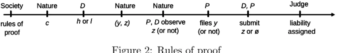
modi…ed as follows. The initial stage, at which was announced, disap-pears. Instead, courts are provided with a set of guiding principles. Moreover, an additional terminal stage is appended at which, if a suit has been …led, the court receives evidence of the form (y; z), y 2 Y , z 2 Z(y) [ f g. Upon receiving that evidence, the court rules whether D caused harm, which by law implies that he is held liable. The court’s decision is denoted by d 2 f0; 1g, where d = 1 means that the defendant pays damages and d = 0 that he does not. If no suit is …led, there is no court action and D does not pay damages.
c Nature h or l D Nature (y, z) Nature P, D observe z (or not) files y (or not) P D, P submit z or ø Society rules of proof liability assigned Judge c Nature c Nature h or l D h or l D Nature (y, z) Nature (y, z) Nature P, D observe z (or not) Nature P, D observe z (or not) files y (or not) P files y (or not) P D, P submit z or ø D, P submit z or ø Society rules of proof Society rules of proof liability assigned Judge liability assigned Judge
Figure 2: Rules of proof
Thus, the game now includes the players D, P and the court as depicted in …gure 2. Everything is assumed to be common knowledge, except D’s cost of care c and his action j 2 fh; lg which are known only to D (the action may also possibly be known to P ), the partial evidence y which is initially known only to D and P , and the additional evidence z 2 Z(y) which is initially known only to D and/or P if they are informed. A party does not know whether the other party observed the additional evidence, neither does the court know whether parties are informed. As before, it is common knowledge that P su¤ers a loss of amount L when D takes action l. Hence, the court’s role is only to assess whether D’s action was h or l.
The complete description of the game requires a speci…cation of the court’s “utility function”. The latter will follow from the rules of proof, as discussed below. The issue is whether, by maximizing its utility, the court is led to assign liability optimally.
Standard of proof and exclusionary rules
The court is taken to be a perfect agent abiding by the rules that the law imposes upon it. Our …rst requirement is for the court to decide the contested
issue on the basis of a “preponderance of evidence”, as this standard of proof is usually understood. The defendant should be found to have caused harm if and only if, upon the evidence, the care level l is more probable than h. As is well known, this is equivalent to requiring that the court minimizes the probability of error. The requirement therefore endows the court with a utility function de…ned by the payo¤s
(d; j) = (
1if d = 0 and j = h or d = 1 and j = l,
0otherwise. (5)
As tie-breaking rule, when h and l are both equally probable, we take it that the court decides against the plainti¤.
We next consider the equilibrium implications of this utility function. Suppose that the parties anticipate d(y; z) = (y; z) for all y 2 Y and z 2 Z(y) [ f g. Party D’s choice of care level, party P ’s decision to …le suit and the outcome of the disclosure game are then the same as before. Denote by Sj(y; z)the equilibrium probability of the outcome “suit is …led and court
receives evidence (y; z)”, conditional on care level j having been exerted. For the case where z 2 Z(y), we have
Sj(y; z) = 8 > < > :
upj(y; z)if (y; z) = 0, (y; ) = 1;
vpj(y; z)if (y; z) = 1, (y; ) = 0;
0 otherwise, where y 2 Y , z 2 Z(y); j = h; l:
(6)
If (y; ) = 1, the plainti¤ sues on the basis of y and has no incentive to submit further evidence; the defendant submits z if he is informed and the additional evidence satis…es (y; z) = 0. The probability for the court to observe (y; z) satisfying the conditions of the top entry is therefore upj(y; z).
When the evidence satis…es the conditions of the middle entry, the plain-ti¤ cannot prevail under y alone. He then sues only if informed and if (y; z) = 1, hence the probability vpj(y; z) that such evidence is
submit-ted. In all other cases, the event “suit is …led and court receives evidence (y; z)” is out-of-equilibrium and its probability is therefore nil. The event is
out-of-equilibrium either because the plainti¤ does not sue or because such a combination of the complete evidence is never submitted when a suit is …led. Bayesian up-dating along the equilibrium path (that is, when Sj(y; z) > 0
for j = h or j = l or both13) implies that, given the complete evidence, the
court’s posterior probability about the defendant’s action is (j j y; z) = 0 jSj(y; z) 0 hSh(y; z) + 0lSl(y; z) = 0 jpj(y; z) 0 hph(y; z) + 0 lpl(y; z) ; j = h; l; z 2 Z(y); (7) where the second equality follows from (6) and where 0
h, 0l = 1 0h denote
the court’s priors at the start of the proceedings. Under the preponderance standard (equivalently, when the court maximizes its expected utility), the defendant is held liable if (l j y; z) > (h j y; z), that is if
0
lpl(y; z) > 0hph(y; z): (8)
Recall that the optimal mechanism generates the deterrence level . Given the distribution function G over the cost of care, this translates into a probability G(L ) that the defendant exerted care. Thus, in equation (7), a Bayesian court would use 0
h = G(L ). Obviously, except nongenerically, a
court adjudicating according to (8) will then not implement the optimal lia-bility assignment, which requires the decision d(y; z) = 1 if pl(y; z) > ph(y; z).
Thus, the preponderance standard does not yield the appropriate out-come. We therefore consider imposing an additional requirement upon court decision-making. This takes the form of “evidentiary rules”. We ask the court to abstract from its knowledge of the cost distribution G and to ap-proach the case with “normative” priors 0
h = 0l = 1
2. The interpretation,
quoting Posner (1999), is that “we want the trier of fact to work with prior odds of 1 to 1 ... that the plainti¤ has a meritorious case”. To illustrate, the
13By assumption, p
h(y; z) + pl(y; z) > 0 for all y 2 Y , z 2 Z(y). Hence, when the
court should put on an “equal” footing defendants drawn from two popula-tions di¤ering by the cost distribution G, hence di¤ering in the actual “prior” probability of having caused harm. In other words, courts should disregard as inadmissible information pertaining to the defendants’reputation for be-having a certain way or to their propensity to act negligently. We refer to the standard of proof and evidentiary rules as the rules of proof.
Clearly, a court abiding by the rules of proof does not minimize the actual probability of error.14 Rather, it is as if it sought to minimize error from the
perspective of an agent holding neutral priors about the individual case upon which it has to decide. Observe that this provides a way out of such classic conundrums as the “bus case” and the “gate crasher’s paradox”. In the latter, 600 of the 1000 people in the audience of a rock concert crashed the gate and did not pay the ticket. Assuming all legitimate ticket stubs have been lost, should someone picked at random in the audience be held liable, given that there is a 60% chance that he was a gate crasher? According to the rules of proof described above, “naked”statistical evidence pertaining to G( ) should simply not be considered.
Proposition 3 The optimal liability assignment d(y; z) = (y; z), y 2 Y , z 2 Z(y) [ f g, is part of an equilibrium with court decision-making con-strained by the rules of proof.
Up to this point we have shown that, under the rules of proof, the court’s decision is consistent with the optimal mechanism when the whole potential evidence is received. To complete the proof of proposition 3, it remains to show that this is also true when the evidence is (y; ) at the close of the proceedings.
In equilibrium, such an outcome occurs only if (y; ) = 1 and the defendant is either uninformed of the true z or gains nothing by submitting
14This contrasts with the justi…cation of the preponderance standard that prevails in
the legal literature (e.g., Sherwin and Clermont, 2002). In a related model, Fluet (2003) compares the ex ante incentives to exert care under truth-seeking courts versus courts abiding by the rules of proof.
the additional evidence because (y; z) = 1 as well. When (y; ) = 0, the outcome (y; ) is not part of the equilibrium because an uninformed plainti¤ does not sue. Taking the above into consideration, the probability of “suit is …led and evidence is (y; )”, conditional on the level of care, is therefore
Sj(y; ) =
(
pj(y)h1 u + uPz2Z(y) (y; z)pj(zj y)
i
if (y; ) = 1; 0otherwise, where y 2 Y , j = h; l:
(9) Along the equilibrium path, using the court’s “normative priors”, the posterior probabilities about the defendant’s action are then
(j j y; ) = (
1
2)Sj(y; )
(12)Sh(y; ) + (12)Sl(y; )
; j = h; l:
Hence, (l j y; ) > (hj y; ) and therefore d(y; ) = 1 if Sl(y; ) >
Sh(y; ). We now show that the latter holds along the equilibrium path.
For this purpose, observe that Qj(y) in proposition 2 can be rewritten as
Qj(y) = 1 u + (u v) X z2Z(y) (y; z)pj(zj y): (10) Substituting in (9), we get Sj(y; ) = pj(y) 2 4Qj(y) + v X z2Z(y) (y; z)pj(z j y) 3 5 ; j = h; l: Therefore,
Sl(y; ) Sh(y; ) = [pl(y)Ql(y) ph(y)Qh(y)]
+ v X
z2Z(y)
(y; z) [pl(y; z) ph(y; z)] > 0:
The sign follows whenever (y; ) = 1, i.e. along the equilibrium path. To see this, observe that by proposition 2, the …rst bracket on the right-hand-side is then positive. Moreover, by proposition 1, the second expression is always nonnegative. Altogether, along the equilibrium path, the court’s decisions under the rules of proof implement the optimal liability assignment. In the appendix we discuss out-of-equilibrium beliefs that sustain the equilibrium.
Multiple equilibria
The foregoing analysis showed that the optimal liability assignment is con-sistent with courts operating on the basis of the preponderance standard and exclusionary rules. Note that the discussion did not refer to the allocation of the burden of proof, although section 4 showed that the optimal mech-anism entails a burden of proof assignment. Under the rules of proof, the appropriate allocation of the burden arose “spontaneously” in the form of presumptions in favor of or against the defendant. Indeed, the argument was that, if the parties’…le and disclosure strategies were the same as under the mechanism , then the court’s best reply would be d = , thereby sustaining the optimal liability assignment as an equilibrium. However, this leaves open the possibility that there are other equilibria, possibly ine¢ cient ones, that are also consistent with the same rules of proof. Speci…cally, if the parties choose their actions under the belief that the court’s strategy is d(y; ) 6= (y; ), can d(y; ) be a best reply for the court?
We illustrate this possibility with the example in Table 1. Recall from section 4 that a party was said to bear the burden of proof if he is the only party with a possible incentive to submit z. In the optimal mechanism for the example of table 1, the defendant bears the burden when u = :8 and v = :6; he is then always held liable when the partial evidence is mixed, which is when y is either af or be. By contrast, the plainti¤ bears the burden when u = :6 and v = :8, since mixed evidence is then not su¢ cient for the plainti¤ to win.
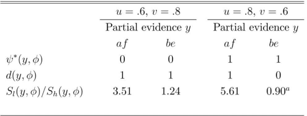
Table 2 reproduces the optimal (y; ) for these two cases. The strat-egy d(y; ), which allocates the burden of proof di¤erently, is also part of a sequential equilibrium consistent with the rules of proof. The table gives d(y; ) only for mixed evidence; in all other cases the court’s decision is the same as .
Table 2: Ine¢ cient Equilibria
u = :6, v = :8 u = :8, v = :6 Partial evidence y Partial evidence y
af be af be
(y; ) 0 0 1 1
d(y; ) 1 1 1 0
Sl(y; )=Sh(y; ) 3.51 1.24 5.61 0.90a
aOut of equilibrium, as described in the text.
To see that d(y; ) as shown is part of an equilibrium, consider …rst the case u = :6, v = :8. In contrast to the optimal liability assignment, it is now as if the court had a presumption against the defendant. The plainti¤ therefore always sues when the evidence is mixed and he never submits z. Since the plainti¤ wins under (y; ), the probability Sj(y; ) is as de…ned
in equation (9) but with d(y; ) substituted for (y; ). Using the …gures in table 1, this yields Sl(y; ) > Sh(y; ). Holding the defendant liable is
therefore warranted under the rules of proof.
When u = :8 and v = :6, the liability assignment under the optimal mechanism is for the defendant to bear the burden of proof. However, in the equilibrium represented in table 2, the defendant prevails when the partial evidence is be. His best response is therefore to remain passive should a suit be …led. Accordingly, an uninformed plainti¤ does not sue when the partial evidence is be since he has nothing to gain (an informed plainti¤ would sue only if the complete evidence is e). Given the court’s strategy, the event “suit is …led and evidentiary outcome is be”is clearly out of equilibrium. In the table, Sl(be; )=Sh(be; ) is derived under the out-of-equilibrium beliefs
that an uninformed plainti¤ sues by mistake with probability ". Hence, conditional on the level of care, the evidence be is presented to the court with probability (1 v)pj(be)". This leads to the posterior odds in table
2.15 Thus, under the rules of proof, the defendant is not held liable, which
sustains the equilibrium.
In both cases, the intuition is the same. An equilibrium is based on self-sustaining presumptions. These a¤ect equilibrium strategies, which in turn a¤ect the inferences that can be drawn from the evidence. Hence, multiple equilibria are possible under the same rules of proof. In the example, all the equilibria are equally reasonable. In fact, the multiplicity of equilibria illustrated in the example is generic, as shown by the next proposition. Proposition 4 Under the rules of proof, there are multiple equilibria if u and v are su¢ ciently large. For any y 2 Y constituting mixed evidence, d(y; ) = 1 is part of one equilibrium and d(y; ) = 0 of another.
When u and v are small, the court’s assessment is essentially determined by whether pl(y) is greater or less than ph(y). The “naive” information
content of y dominates since the parties are relatively unlikely to possess additional information. Hence, the equilibrium is unique. By contrast, when uand v are large, the interpretation of (y; ) is equilibrium determined, hence the existence of multiple equilibria.
Burden of proof and active judges
This suggests a role for additional judicial tools in order to help select the right equilibrium. One possibility is to provide courts with guidelines re-garding the allocation of the burden of proof. For instance, suppose there is a category of cases corresponding to u = :6 and v = :8. For this category, courts could be instructed to let the plainti¤s bear the burden.
15These are the same as the “uncorrected” odds in table 1. There are other
possibil-ities. The court could rationalize the out-of-equilibrium outcome as a suit by either an uninformed plainti¤ or an informed one with unfavorable evidence. This would lead to even smaller posterior odds Sl=Sh. The equilibrium is sustained as long as the court does
not put too much weight on the possibility that an informed plainti¤ sued on the basis of favorable complete evidence, but then “forgot” to submit z.
An interpretation is that courts are then required to use a speci…c pre-sumption. In terms of the model, the guideline could also be interpreted as a statement to the e¤ect that a plainti¤ can prevail only if he also submits the second “…le”(which contains z). This amounts to specifying the type of evidence required to win a suit, i.e., it characterizes the necessary conditions for a “proof”. Such guidelines could be imposed through statute law or follow from rulings by higher jurisdictions. They could also derive from custom or general jurisprudence. Whatever the means, the important point is that the burden assignment does not follow from the rules of proof alone at the trial court level. Obviously, burden of proof guidelines must apply to large classes of cases, irrespective of the detailed information only available at the court level. In general, they will therefore not be su¢ cient to ensure coordination on the e¢ cient equilibrium.
In the remainder we consider another possibility. So far, our stylized court procedure involved a purely “passive”adjudicator whose only role is to decide at the close of the proceedings, once the parties have presented evidence favouring their case. We now allow the adjudicator to intervene during the proceedings, as in the more inquisitorial procedure of civil law countries. By contrast with a purely adversarial (i.e., party controlled) procedure, where the judge sits as a silent referee, the “inquisitorial judge” interrogates the parties or witnesses directly and may purposely shift the burden of proof. In civil litigation, the more or less active role of the judge is one of the main di¤erences between the common law and civil law procedures, since most if not all of the evidence is supplied by the parties in both systems.
We model the active court as follows. As before, the court’s decision is d(y; z), for y 2 Y and z 2 Z(y) [ f g, at the close of the proceedings. However, the game is augmented to include an intermediate stage, after the plainti¤’s decision to …le suit and the presentation of y and before the poten-tial disclosure of additional evidence. At this intermediate stage, the judge interrogates the parties for possible additional evidence and may suggest how he would rule on the basis of the evidence presented so far. Formally, the
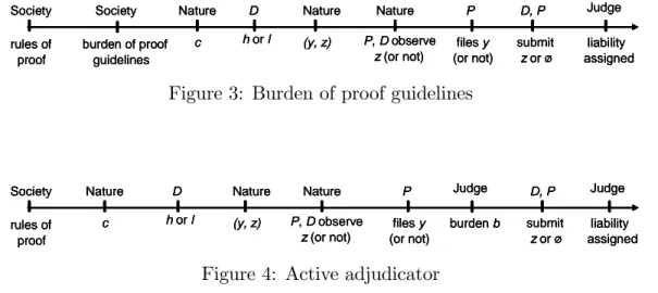
judge makes an announcement b 2 f0; 1g, where b = 1 means “su¢ cient”, i.e., it conveys that the plainti¤ will prevail on the basis of the evidence y alone unless additional evidence is brought forward by the defendant. In other words, b = 1 suggests that the burden of proof is on the defendant and is equivalent to interrogating the defendant under the threat of adjudicat-ing against him. Conversely, b = 0 means “insu¢ cient” and suggests that the burden of proof is still on the plainti¤. The …gures 3 and 4 emphasize the di¤erence between burden of proof guidelines imposed “from above”and burden of proof shifts through announcements at the trial court level.
c Nature h or l D Nature (y, z) Nature P, D observe z (or not) files y (or not) P D, P submit z or ø Society rules of proof liability assigned Judge Society burden of proof guidelines c Nature c Nature h or l D h or l D Nature (y, z) Nature (y, z) Nature P, D observe z (or not) Nature P, D observe z (or not) files y (or not) P files y (or not) P D, P submit z or ø D, P submit z or ø Society rules of proof Society rules of proof liability assigned Judge liability assigned Judge Society burden of proof guidelines Society burden of proof guidelines
Figure 3: Burden of proof guidelines
c Nature h or l D Nature (y, z) Nature P, D observe z (or not) files y (or not) P D, P submit z or ø Society rules of proof liability assigned Judge burden b Judge c Nature c Nature h or l D h or l D Nature (y, z) Nature (y, z) Nature P, D observe z (or not) Nature P, D observe z (or not) files y (or not) P files y (or not) P D, P submit z or ø D, P submit z or ø Society rules of proof Society rules of proof liability assigned Judge liability assigned Judge burden b Judge burden b Judge
Figure 4: Active adjudicator
We …rst consider the case where announcements are binding. To illus-trate, in German civil procedure, the judge may inform a party that, unless he presents some additional more convincing evidence, the court is likely to rule a certain way. Such a “judicial advice”is written to the protocol of the proceeding, which in general would make it di¢ cult for a judge not to follow through (otherwise a mislead party would have ground for appeal).16 We show that, if judicial announcements are binding and the judge otherwise abides by the rules of proof, there is a unique equilibrium characterized by
the optimal liability assignment. We next consider non binding announce-ments. The communication stage is then purely rhetorical, involving cheap talk. We show that the same results nevertheless follow if one assumes that “credible” announcements are believed by the parties.
Denote by b(y) the judge’s announcement strategy, i.e., the announcement at the information set where a suit has been …led and he partial evidence is y. When announcement are binding, decisions at the terminal adjudication stage are constrained by d(y; ) = b(y). We have the following result.
Proposition 5 If the judge’s announcements are binding, the equilibrium is unique and the judge’s strategy under the rules of proof satis…es b(y) = (y; ), d(y; ) = b(y), d(y; z) = (y; z), y 2 Y , z 2 Z(y).
Given the rules of proof, the judge and the parties know that d(y; z) = (y; z) will be chosen if the complete evidence is disclosed. Faced with a binding announcement, the parties have dominant strategies regarding dis-closure. Anticipating the parties’response, the judge therefore chooses b to maximize his expected payo¤ (the probability of not making “mistakes”), us-ing the “normative”priors about the defendant’s care level and conditionally on his beliefs at the information set y. These beliefs do not depend on the parties’s strategies, hence the equilibrium is unique.
We now extend the analysis to non binding announcements. As is well known from the cheap talk literature, there always exists an equilibrium where costless statements are considered to be meaningless. In the present context, this would mean that the outcome of the game with inquisitorial judge is the same as with a passive adjudicator. In what follows, we select equilibria satisfying the condition that credible statements about planned behavior are believed. Standard requirements for credibility are that an-nouncements be self-committing and self-signalling (see for instance Farrell and Rabin, 1996).
Consider the …rst requirement. At the information set y, the announce-ment b is self-committing when d(y; ) = b is the judge’s best response at
the adjudication stage, if he expects the announcement to be believed. This requires that d(y; ) be part of an equilibrium. From proposition 3, it fol-lows that the announcement b = (y; ) is self-committing. In particular, when the game with passive adjudicator has a unique equilibrium, then the only credible announcements are those which yield the optimal liability as-signment. However, from proposition 4, we know that there are cases where d(y; ) 6= (y; ) is also part of an equilibrium. Hence, an announcement b0 6= (y; ) would also be self-committing, although by proposition 5 the
judge would prefer to announce b and carry out his plan if he expected b to be believed.
However, a judge announcing b may still be tempted to adjudicate ac-cording to b0 if he thinks the announcement of b will not be believed. In
particular, a di¢ culty arises if the payo¤ from adjudicating according to b0 is
greater when the parties play under the belief that the judge will stick to b. Knowing this, it could be rational for the parties not to believe b. The self-signalling requirement is an additional condition ruling out this di¢ culty.17
Announcements are self-signalling if the judge would not want the parties to believe he will play some b00 if he intends to play otherwise, i.e., if he has no
incentive to be misleading about his intentions, whatever these are. We show that this requirement is satis…ed.
Lemma 2 The judge’s announcements of d(y; ) are self-signalling.
Given the self-signalling property, self-committing announcements should therefore be believed. The next result then follows directly from proposi-tion 5.
Proposition 6 Under the rules of proof, d(y; z) = (y; z), y 2 Y , z 2 Z(y) [ f g, is part of the unique equilibrium satisfying the condition that credible announcements are believed.
17The condition is due to Aumann (1990). Baliga and Morris (2002) provide an
6
Related literature and conclusions
Posner (1999) remarked that the economic literature on the law of evidence is scanty in relation to its scope and importance. While there is an already vast literature on litigation, the legal principles constraining court decision-making have been little discussed from the usual standpoint of law and eco-nomics. Our contribution has been to provide a simple model to analyze some of the basic issues concerning rules of proof and procedures. We sum-marize our main results, relate them to the literature and suggest possible extensions.
It has been emphasized elsewhere (in particular Daughety and Reinganum 2000a, 2000b) that the trial process cannot be purely Bayesian due to eviden-tiary rules and other features of the procedure. It has also often been noted that it may be useful to commit Bayesian decision-makers to rules that may not be optimal ex post from an error-minimizing perspective (e.g., Schrag and Scotchmer 1994, Daughety and Reinganum 1995, Lewis and Poitevin 1997, Sanchirico 2001b, Bernhardt and Nosal 2004). We showed that, if the purpose of tort law is deterrence, the preponderance standard and the usual exclusionary rules under common law are e¢ cient. An extension would be to dwell deeper into the characterization of courts as “constrained-Bayesians” and consider rules of proof in more complex litigation.
The trial was modelled as a persuasion game in the manner of Milgrom and Roberts (1986), assuming that the extent of the interested parties’infor-mation is not veri…able, as in Shin (1998). One di¤erence with the latter is that there are typically multiple equilibria in our set-up, which explains the need for burden of proof guidelines or for a more active judge. Multiple equi-libria arise non trivially because of our assumption that presenting evidence is costly, so that parties have no incentives to submit favorable evidence un-less it strictly improves their prospects. Similar results were also obtained by Sobel (1985) in a model where proofs are costly. We showed that an ac-tive judge, operating under common law rules of proof, would allocate the burden of proof e¢ ciently. Even if burden of proof announcements are not
binding, the active judge can elicit e¢ cient disclosure by credibly threatening the parties to adjudicate a certain way.
These results shed light on the adversarial versus inquisitorial controversy. The distinction refers to the role of the judge versus the parties’in the fact-…nding phase of the trial, with common law on the one hand and civil law on the other. In the economic literature, “inquisitorial” has usually been assimilated to a procedure where a disinterested investigator (e.g., a public o¢ cial) is responsible for discovery, as opposed to the adversarial method where the parties have full control over the uncovering and presentation of evidence (see Shin 1998, Dewatripont and Tirole 1999, Froeb and Kobayashi 2001, Palumbo 2001).18 However, as far as civil litigation is concerned and by
contrast with criminal trials, the presentation of proof is mainly the parties’ responsibility even in the civil law system.
While the civil law judge may investigate facts on his own initiative (e.g., through court-appointed experts), the main practical di¤erence is the judge’s greater direct involvement in guiding the litigants’ submission of evidence through bench request, questions and suggestions (Parisi, 2002, provides a short comparative description). This is not unlike “managerial judging” in the US discovery process, in the sense that it may focus discovery (and pre-vent excesses, see Schrag 1999), but it does also allow the use of hints or threats, implicit or explicit, as to how the judge will adjudicate on the basis of the evidence presented so far. If the extent of the parties’information is unveri…able, such threats may be the only means available to elicit disclosure. Our analysis provides a rationale for a procedure with an active judge.19
18One exception is Block and Parker’s (2004) experimental study of the e¢ ciency of
adjudication with a passive referre as opposed to an active one who is the only ques-tioner permitted. They interpret their …ndings as suggesting the need for burden of proof guidelines in the purely adversarial procedure.
19Actual systems range on a scale from the theoretically pure adversarial to the
theoret-ically pure inquisitorial (see Jolowicz, 2000, 2003). For instance, article 32.1 of England’ new Civil Procedure Rules allows the court much power in controlling evidence. Sim-ilarly, under Rule 614(b) of the Federal Rules of Evidence, U.S. federal courts may in principle interrogate and even call witnesses, although in practice this is unusual. On the
Our results would be a¤ected if society is also concerned with the costs of presenting evidence. Bernardo, Talley and Welch (2000) analyzed the trade-o¤ between deterrence and litigation costs (see also Rubinfeld and Sapping-ton, 1987). A similar concern in our model would seem to justify a more stringent standard of proof than preponderance. This would yield less de-terrence but would also reduce the frequency of suits, and thereby litigation costs, by making it more di¢ cult for a plainti¤ to prevail. A concern for costs would also impact on the allocation of the burden of proof if parties di¤er in the cost of presenting the “additional” evidence, i.e., there would now be a tendency to put the burden on the cheaper information provider (see Hay and Spier, 1997), although taking into account the likelihood that the litigants have access to evidence. This would a¤ect disclosure, hence deterrence.
However, changes in the standard of proof and in the allocation of the burden of proof interact in complex ways. Allocating the burden of proof to the defendant because he is the cheaper information provider could stimulate suits. Moreover, if the defendant is allocated the burden of proof for cost reasons, must he meet the same higher standard of proof to discharge it, which would also stimulate suits? Whether reasonably simple general rules of proof can be obtained in this context is doubtful but merits future research. We abstracted from many other relevant considerations. For instance, our litigants were endowed with hard evidence. Their strategies would be di¤erent if they had to invest to uncover evidence. How does this impact on the e¢ cient standard of proof and burden assignment? We also abstracted from the possibility of out-of-court settlements. Again, this is an avenue for future research.
other hand, judicial or statutory decisions in most U.S. states have explicitly restricted the judge’s power to comment on the evidence.
Appendix
Proof of proposition 2: We …rst justify the expression for ej(y) in (2).
Let Z+(y) Z(y) be the set of z’s such that (y; z) > (y; ). Similarly, let Z (y) Z(y) be the set of z’s such that (y; z) < (y; ). An informed plainti¤ submits z only if z 2 Z+(y); an informed defendant submits z only if z 2 Z (y). Then ej(y) = 0 @1 v X z2Z+(y) pj(zj y) u X z2Z (y) pj(zj y) 1 A (y; ) + v X z2Z+(y) pj(zj y) (y; z) + u X z2Z (y) pj(zj y) (y; z): (11)
To see this, note that the expression in the right-hand side parenthesis equals 0 @1 X z2Z+(y) pj(zj y) X z2Z (y) pj(zj y) 1 A + (1 v) X z2Z+(y) pj(z j y) + (1 u) X z2Z (y) pj(zj y):
This is the probability that additional evidence will not change the prob-ability of liprob-ability compared to (y; ), plus the probprob-ability that it would have but the interested party was uninformed. Hence, it is the probability of “no change”. The second term in (11) is the probability that the plainti¤ is informed times the expected probability of liability for z 2 Z+(y). A similar
interpretation holds for the third term. Expression (11) can be rewritten as
ej(y) = (y; ) + v
X
z2Z+(y)
pj(zj y) (y; z) [ (y; z) (y; )]
u X
z2Z (y)
which explains (2).
The optimal maximizes deterrence de…ned as
= X
y2Y
[pl(y)el(y) ph(y)eh(y)]
= X
y2Y
[pl(y) ph(y)] (y; ) +X
y2Y
X
z2Z(y)
[pl(y; z) ph(y; z)] (y; z); (12)
where we substituted for ej(y) from (2) and where
(y; z) = v max[0; (y; z) (y; )] u max[0; (y; ) (y; z)]: (13) The second term in (12) is maximized if (y; z) is as large as possible when pl(y; z) > ph(y; z) and as small as possible when pl(y; z) < ph(y; z).
Taking (y; ) as given, this implies (y; z) =
(
1 when pl(y; z) > ph(y; z);
0 when pl(y; z) < ph(y; z):
Thus, (y; z) = (y; z) for z 2 Z(y), which proves the …rst claim in the proposition. Substituting this result in (13) and from the latter in (12) yields
= X
y2Y
[pl(y) ph(y)] (y; )
+X
y2Y
X
z2Z(y)
[pl(y; z) ph(y; z)]v (y; z)(1 (y; ))
X
y2Y
X
z2Z(y)
[pl(y; z) ph(y; z)]u(1 (y; z)) (y; )
= vX
y2Y
X
z2Z(y)
[pl(y; z) ph(y; z)] (y; z)
+X
y2Y
where Qj(y) = 1 v X z2Z(y) (y; z)pj(zj y) u X z2Z(y) [1 (y; z)]pj(zj y) or equivalently Qj(y) = (1 v)(1 u) + (1 u)v X z2Z(y) [1 (y; z)]pj(zj y) + (1 v)u X z2Z(y) (y; z)pj(zj y):
Choosing (y; ) to maximize the second term in (14) implies (y; ) =
(
1 when pl(y)Ql(y) > ph(y)Qh(y);
0 when pl(y)Ql(y) < ph(y)Qh(y);
thereby proving the second claim.
Proof of corollary 2: The optimal scheme assigns liability according to the sign of
(y) := pl(y)Ql(y) ph(y)Qh(y) = (1 v) +(y) + (1 u) (y) (15)
where
+(y) := X z2Z(y)
(y; z)[pl(y; z) ph(y; z)] > 0; (16)
(y) := X
z2Z(y)
[1 (y; z)][pl(y; z) ph(y; z)] 0; (17)
and where the sign follows from proposition 2 and the assumption that y is mixed. To prove the …rst part of the corollary, recall that the burden is on the defendant if (y) > 0. Now, (y) > 0 when v < u = 1. By continuity, it follows that there exists uc 2 (v; 1) such that (y) > 0 if u uc. The proof
of the second part is similar provided (y) < 0, which obtains if there exists z 2 Z(y) such that pl(y; z) < ph(y; z).