2019 — Finite and discrete element modelling of internal erosion in water retention structures

Finite and Discrete Element Modelling of Internal Erosion in

Water Retention Structures

by

Seyed Pouyan PIRNIA

MANUSCRIPT-BASED THESIS PRESENTED TO ÉCOLE DE

TECHNOLOGIE SUPÉRIEURE IN PARTIAL FULFILLMENT OF THE

REQUIREMENTS FOR THE DEGREE OF DOCTOR OF PHILOSOPHY

Ph.D.

MONTREAL, JULY 19, 2019

ÉCOLE DE TECHNOLOGIE SUPÉRIEURE

UNIVERSITÉ DU QUÉBEC

This Creative Commons licence allows readers to download this work and share it with others as long as the author is credited. The content of this work can’t be modified in any way or used commercially.

BOARD OF EXAMINERS

THIS THESIS HAS BEEN EVALUATED BY THE FOLLOWING BOARD OF EXAMINERS

Mr. François Duhaime, Thesis Supervisor

Department of Construction Engineering at École de technologie supérieure

Mr. Yannic A. Ethier, Thesis Co-supervisor

Department of Construction Engineering at École de technologie supérieure

Mr. Philippe Bocher, President of the Board of Examiners

Department of Mechanical Engineering at École de technologie supérieure

Mr. Henri Champliaud, Member of the jury

Department of Mechanical Engineering at École de technologie supérieure

Mr. Mohamed Meguid, External Evaluator

Department of Civil Engineering at McGill University

THIS THESIS WAS PRESENTED AND DEFENDED

IN THE PRESENCE OF A BOARD OF EXAMINERS AND PUBLIC JULY 3, 2019

ACKNOWLEDGMENT

My special acknowledgments are for my advisor, Prof. François Duhaime, for his guidance, strong passion, encouragement and flexibility that made this dissertation possible. This dissertation would not have been possible without his scientific contribution. I have had the chance to be accepted in his research group and worked with such a wonderful man. I must thank my co-advisor Prof. Yannic Ethier for his invaluable support and kindly advice during my doctoral works. I am also deeply thankful to Prof. Jean-Sébastien Dubé for his contribution as a co-author in the papers.

I would like to thank the PhD committee members: Dr. Mohamed Meguid, Dr. Henri Champliaud and Dr. Philippe Bocher for their valuable time in reviewing the dissertation. Many thanks go to the experts in Hydro-Québec, especially Annick Bigras and Hugo Longtin. The thesis could not be completed without financial support from Hydro-Québec and NSERC.

I would like to acknowledge all my friends and teachers who supported me during my journey from Iran to Canada, especially Bahram Aghajanzadeh. Thanks to my LG2 colleagues who have enriched my daily life throughout my studies.

I would highly indebt to my dear parents for their endless love, dedication and support in my life. They always got my back and helped me to fulfill my dreams. My special thanks are extended to my brother, Amir, for his support and guidance. Finally, I have to thank my beloved wife, Sadaf, for her love, understanding and encouragement which helped in completion of this thesis.

Modélisation par éléments finis et éléments discrets de l'érosion interne dans les ouvrages de rétention d'eau

Seyed Pouyan PIRNIA RÉSUMÉ

L'érosion interne implique le transport de particules à l’intérieur d'un sol en raison d'un écoulement en milieu poreux. Ce phénomène est considéré comme une menace sérieuse pour les structures en matériaux granulaires. L’érosion interne est la principale cause de dommage ou de rupture du corps ou de la fondation des barrages en remblai. Par conséquent, il est nécessaire d’avoir une connaissance précise des interactions fluide-particule dans les sols saturés lors de la conception et de l’exploitation des barrages. Le comportement hydrodynamique des milieux poreux en géotechnique est généralement modélisé à l'aide de méthodes qui considèrent le sol comme un milieu continu, telles que la méthode des éléments finis (MEF).

Il est de plus en plus courant de combiner la méthode des éléments discrets (MED) avec des méthodes pour les milieux continus, comme la MEF, afin de fournir des informations microscopiques sur les interactions fluide-solide. Cette thèse a pour but de développer un algorithme MEF-MED hiérarchique permettant d'analyser le processus d'érosion interne dans des milieux poreux pour des applications à grande échelle. Pour atteindre cet objectif, nous avons (i) programmé une interface polyvalente entre deux codes MEF et MED, (ii) développé une méthode macroscopique de calcul des forces de trainée sur les particules (CGM) pour le modèle couplé MEF-MED afin de minimiser le temps de calcul, (iii ) développé un algorithme multi-échelle pour l'interface afin de limiter le nombre de particules discrètes impliquées dans la simulation, (iv) évalué la précision de la force de traînée dérivée de CGM, et (v) former un réseau de neurones artificiels (ANN) afin d'améliorer la prédiction de la force de traînée sur les particules.

Le développement de modèles multiméthodes ou hybrides combinant des analyses de type continuum et des éléments discrets est une piste de recherche prometteuse pour combiner les avantages associés aux deux échelles de modélisation. Cette thèse présente tout d’abord ICY, une interface entre COMSOL Multiphysics (code commercial d’éléments finis) et YADE (code d’éléments discrets ouvert). À travers une série de classes JAVA, l’interface associe la modélisation par éléments discrets à l’échelle des particules à la modélisation à grande échelle avec la méthode des éléments finis. ICY a été validé avec un exemple simple basé sur la loi de Stokes. Une comparaison des résultats pour le modèle couplé et la solution analytique montre que l'interface et son algorithme fonctionnent correctement. Le chapitre présente également un exemple d'application pour l'interface. L’interface a utilisé la force de traînée CGM pour modéliser un test d’érosion interne dans un perméamètre.

Le nombre de particules qui peuvent être incluses dans les simulations DEM avec ICY est limité. Cette limitation réduit le volume de sol pouvant être modélisé. La deuxième partie de la thèse propose une approche multiméthode hiérarchique basée sur ICY pour modéliser le comportement couplé hydromécanique de sols granulaires saturés. Un algorithme multiméthode a été développé pour limiter le nombre de particules dans la simulation DEM et permettre à terme la modélisation de l'érosion interne de grandes structures. Le nombre de particules dans les simulations a été limité en utilisant des sous-domaines discontinus le long de l'échantillon. Cette approche évite de générer le domaine complet comme modèle DEM. Les particules dans ces petits sous-domaines ont été soumises à la flottabilité, à la gravité, à la force de traînée et aux forces de contact pendant de courts pas de temps. Les petits sous-domaines fournissent au modèle de continuum des données initiales (par exemple, un flux de particules). Le modèle FEM résout une équation de conservation des particules pour évaluer les changements de porosité sur des intervalles de temps plus longs. L’algorithme multi-échelle a été vérifié en simulant un test numérique d’érosion interne.

Le mouvement des fluides dans les applications géotechniques est généralement résolu avec une forme homogénéisée des équations de Navier-Stokes. La force totale de traînée obtenue de la CGM peut être appliquée aux particules proportionnellement à leur volume (CGM-V) ou à leur surface (CGM-S). Cependant, il existe une certaine incertitude quant à l’application des modèles de traînée CGM aux mélanges polydisperses de particules. La précision de CGM pour la modélisation de n'a pas été systématiquement étudiée en comparant les résultats CGM avec les résultats plus précis obtenus en résolvant les équations de Navier-Stokes à l'échelle des pores. La dernière partie de cette thèse compare les forces de traînée CGM-V et CGM-S avec celles qui sont obtenues avec la résolution des équations de Navier-Stokes à l’échelle des pores avec la MEF. COMSOL Multiphysics a été utilisé pour simuler l'écoulement dans trois cellules unitaires avec différentes valeurs de porosité (0,477, 0,319 et 0,259). Chaque cellule unitaire comportait un squelette monodisperse de grandes particules avec des positions fixes, et une particule plus petite, de taille et de position variables. Les résultats ont montré que les forces de trainée CGM-V et CGM-S sont généralement assez éloignées des forces obtenues à petite échelle avec la MEF. La précision diminue davantage quand le contraste entre les tailles des grandes particules et de la petite particule augmente. Un ANN a été formé pour prédire la force de trainée MEF en utilisant comme données d’entrée les forces de trainée CGM-V et CGM-S, le rapport entre les tailles de particules, et la distance entre la petite particule et les deux grandes particules les plus près. Une très bonne corrélation a été trouvée entre la sortie de l’ANN et les résultats MEF. Ce résultat montre qu'un ANN peut fournir des forces de trainée aussi précises que celles de la MEF, mais avec un temps de calcul comparable à celui des méthodes CGM. Cette thèse contribue à la littérature en améliorant notre compréhension des méthodes hybrides MED-continuum et des calculs de force de traînée dans les simulations MED. La thèse présente des recommandations aux chercheurs et aux développeurs qui tentent de modéliser l'érosion interne dans des systèmes de sols à l'échelle réelle.

Mots-clés: érosion interne, élément discret, élément fini, COMSOL, YADE, force de traînée, calcul macroscopique des forces de trainée, réseau de neurones artificiels

Finite and Discrete Element Modelling of Internal Erosion in Water Retention Structures

Seyed Pouyan PIRNIA ABSTRACT

Internal erosion is a process by which particles from a soil mass are transported due to an internal fluid flow. This phenomenon is considered as a serious threat to earthen structures. Internal erosion is the main cause of damage or failure in the body or foundation of embankment dams. Therefore, it is necessary to have an accurate knowledge of fluid-particle interactions in saturated soils during design and operation. The hydrodynamic behaviour of porous media in geotechnical engineering is typically modelled using continuum methods such as the finite element method (FEM).

It has become increasingly common to combine the discrete element method (DEM) with continuum methods such as the FEM to provide microscopic insights into the behaviour of granular materials and fluid–solid interactions. This Ph.D. thesis aims to develop a hierarchical FEM-DEM algorithm to analyze the internal erosion process in large scale earthen structures. To achieve this goal, we (i) programmed a versatile interface between two FEM and DEM codes, (ii) implemented a coarse-grid method (CGM) for the coupled FEM-DEM model to minimize the computations associated with drag force calculation, (iii) developed a multiscale algorithm for the interface to limit the number of discrete particles involved in the simulation, (iv) assessed the accuracy of drag force derived from CGM, and (v) trained an Artificial Neural Network (ANN) to improve the prediction of the drag force on particles.

The development of multimethod or hybrid models combining continuum analyses and discrete elements is a promising research avenue to combine the advantages associated with both modelling scales. This thesis first introduces ICY, an interface between COMSOL Multiphysics (commercial finite-element engine) and YADE (open-source discrete-element code). Through a series of JAVA classes, the interface combines DEM modelling at the particle scale with large scale modelling with the finite element method. ICY was verified with a simple example based on Stokes’ law. A comparison of results for the coupled model and the analytical solution shows that the interface and its algorithm work properly. The thesis also presents an application example for the interface. The interface used CGM drag force to model an internal erosion test in a permeameter.

The number of particles that can be included in the DEM simulation of ICY is limited, thus restricting the volume of soil that can be modelled. The second part of the thesis proposes a multimethod hierarchical approach based on ICY to model the coupled hydro-mechanical behaviour for saturated granular soils. A hierarchical algorithm was specifically developed to limit the number of particles in the DEM simulations and to eventually allow the modelling of internal erosion for large structures. The number of discrete bodies in the simulations was

restricted through employing discontinuous subdomains along the sample. This avoids generating the full sample as a DEM model. Particles in these small subdomains were subjected to buoyancy, gravity, drag force and contact forces for small time steps. The small subdomains provide the continuum model with particle flux. The FEM model solves a particle conservation equation to evaluate porosity changes for longer time steps. The multimethod framework was verified by simulating a numerical internal erosion test.

The fluid motion in geotechnical applications is typically solved using CGM. With these methods, an average form of the Navier–Stokes equations is solved. The total drag force derived from CGM can be applied to the particles proportionally to their volume (CGM-V) or surface (CGM-S). However, there is some uncertainty regarding the application of the CGM drag models for polydispersed particle. The accuracy of CGM has not been systematically investigated through comparing CGM results with more precise results obtained from solving the Navier-Stokes equations at the pore scale. The last part of this research investigates the accuracy of CGM-V and CGM-S drag forces in comparison with the pore-scale values obtained by FEM. COMSOL Multiphysics was used to simulate the fluid flow in three unit cells with different porosity values (0.477, 0.319 and 0.259). The unit cell involved a mono-size skeleton of large particles with fixed positions and a smaller particle with variable mono-sizes and positions. The results showed that the CGM-V and CGM-S could not predict precisely the drag force on the small particle. An ANN was trained to predict the drag force on the smaller particle. A very good correlation was found between the ANN output and the FEM results. The ANN could thus provide drag force values with accuracy similar to that obtained using flow simulations at the pore scale, but with computational resources that are comparable to CGM. This thesis contributes to the literature by improving our understanding of hybrid DEM-continuum methods and drag force computations in DEM simulations. It provides guidelines to researchers and developers who try to model internal erosion in real scale soil systems.

Keywords: Internal erosion, discrete element, finite element, COMSOL, YADE, drag force, coarse-grid method, artificial neural network

TABLE OF CONTENTS

Page

CHAPTER 1 INTRODUCTION ...1

1.1 Background ...1

1.2 Objectives ...7

1.3 Synopsis and content...8

CHAPTER 2 LITERATURE REVIEW ...11

2.1 Physics of porous media ...11

2.2 Internal erosion ...13

2.3 Numerical modelling of fluid-particle interaction ...17

2.3.1 Fluid transport equations in porous media ... 19

2.3.2 Discrete Element Method ... 24

2.3.2.1 Governing equations of motion ... 26

2.3.2.2 Constitutive models ... 30

2.3.2.3 Damping ... 35

2.3.2.4 Numerical stability ... 36

2.3.2.5 DEM applications in geotechnical engineering ... 37

2.3.2.6 YADE framework ... 39

2.3.3 Coupling DEM-flow schemes... 41

2.4 Numerical modelling of internal erosion in embankment dams ...43

2.5 Multiphysics models ...47

CHAPTER 3 ICY: AN INTERERFACE BETWEEN COMSOL MULTIPHYSICS AND YADE ...49

3.1 Abstract ...49

3.2 Introduction ...50

3.3 Methodology ...54

3.3.1 COMSOL and YADE ... 54

3.3.2 Coupling procedure ... 55

3.4 Verification ...57

3.4.1 Fall velocity and Stokes’ equation ... 57

3.4.2 YADE model ... 59

3.4.3 COMSOL model ... 59

3.4.4 Verification results ... 60

3.5 Application example ...61

3.5.1 Apparatus, testing materials and procedure ... 61

3.5.2 Fluid-DEM coupling theory ... 62

3.5.3 Model implementation ... 66

3.5.4 Calculation sequence ... 69

3.6 Application results and discussion ...71

CHAPTER 4 HIERARCHICAL MULTISCALE NUMERICAL MODELLING OF

INTERNAL EROSION WITH DISCRETE AND FINITE ELEMENTS 75

4.1 Abstract ...75

4.2 Introduction ...76

4.3 Methodology ...81

4.3.1 ICY ... 81

4.3.2 Hierarchical multiscale FEM-DEM model ... 81

4.3.2.1 DEM ... 83

4.3.2.2 FEM and computation cycle ... 85

4.4 Validation example ...88

4.4.1 Full specimen model implementation ... 90

4.4.2 Hierarchical multiscale model implementation ... 91

4.5 Results and Discussions ...94

4.5.1 Full specimen model ... 94

4.5.2 Hierarchical multiscale model (HMM) ... 97

4.6 Conclusion ...102

CHAPTER 5 DRAG FORCE CALCULATIONS IN POLYDISPERSE DEM SIMULATIONS WITH THE COARSE-GRID METHOD: INFLUENCE OF THE WEIGHTING METHOD AND IMPROVED PREDICTIONS THROUGH ARTIFICIAL NEURAL NETWORKS ...103

5.1 Abstract ...103

5.2 Introduction ...104

5.3 Coarse-grid method ...108

5.4 Methodology ...112

5.4.1 FEM model development and drag force calculations ... 112

5.4.2 Artificial Neural Network ... 115

5.5 Results and discussion ...119

5.6 Conclusions ...125

CHAPTER 6 CONCLUSIONS AND RECOMMENDATIONS ...127

6.1 Conclusions ...127

6.2 Recommendations ...134

APPENDIX I ICY INSTRUCTION GUIDE ...137

APPENDIX II VERIFICATION CODES ...147

APPENDIX Ⅲ APPLICATION EXAMPLE CODES ...159

LIST OF FIGURES

Figure 1.1 Homogeneous earth dam with chimney drain (a) and Zoned earth dam with

central vertical core (b) ...1

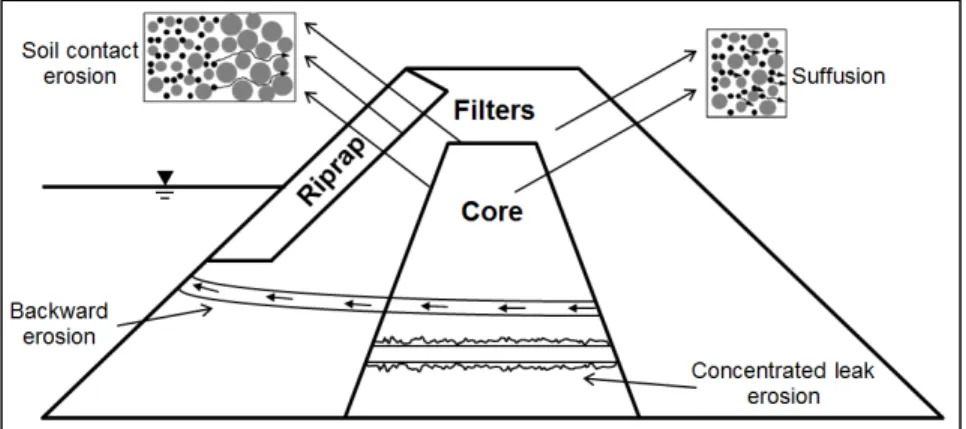
Figure 1.2 Backward erosion, concentrated leak, suffusion and soil contact erosion ...4

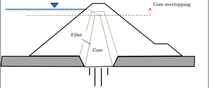
Figure 1.3 Core overtopping and water flow at the interface of core and filter ...5

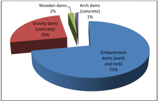
Figure 1.4 Percentage of dams operated by Hydro-Québec according to their type ...6

Figure 2.1 Example of a 3D porous medium ...12

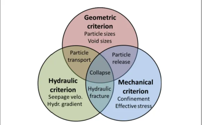
Figure 2.2 Conceptual diagram of internal erosion criteria ...15

Figure 2.3 Calculation sequences in a DEM simulation ...25

Figure 2.4 Geometry of the contact of two spheres ...28

Figure 2.5 Rheological contact model ...29

Figure 2.6 Sandglass experimental setup ...33

Figure 2.7 Experimental and numerical modeling of the repose angle tests: (a) tetrahedral clumps; (b) cubic clumps; (c) octahedral clumps; (d) sphere; (e) & (f) experimental observations ...34

Figure 2.8 Layered structure of YADE framework ...40

Figure 2.9 Simplified schematics of simulation loop ...40

Figure 2.10 Schematic of hierarchical multiscale modelling ...46

Figure 3.1 Schematic view of the ICY algorithm in the context of the verification example 56 Figure 3.2 Comparison of terminal velocity and accelerations through Stokes’ law and FEM-DEM model ...60

Figure 3.3 Schematic diagram of laboratory permeameter ...62

Figure 3.4 Effective forces on water in a volume of porous media ...65

Figure 3.5 Model implementation in COMSOL and YADE. The x coordinate in COMSOL (b) represents the vertical axis in YADE (a) ...66

Figure 3.7 Eroded mass for the experimental test, FEM-DEM model with different

parameters and DEM under constant drag force ...71

Figure 4.1 Representation of the numerical specimen for the modelling of suffusion ...82

Figure 4.2 Effective forces on water in a DEM subdomain ...83

Figure 4.3 Change in small particle flux for a porous media RVE...86

Figure 4.4 Example of time steps for COMSOL and YADE in the hierarchical multiscale model. Both water and particle conservation equations are solved for longer time steps in the COMSOL model. Flux values are computed for shorter time steps in YADE ...87

Figure 4.5 Model implementation in YADE and COMSOL for the full specimen procedure . ...90

Figure 4.6 Model implementation in YADE and COMSOL for the hierarchical multiscale model. All particles (a) or only the coarse particles (b) are kept below the flux calculation section ...92

Figure 4.7 Calculation sequence in the hierarchical multiscale simulations ...93

Figure 4.8 Particle flux as a function of time for two time steps of 0.012 s(a) and 0.05 s(b) .95 Figure 4.9 Cumulative eroded mass for the full specimen procedure and the reference hierarchical multiscale model (HMM). ...96

Figure 4.10 Flux and porosity in the DEM cells or subdomains as a function of time elapsed since the simulation beginning for the full specimen procedure and the reference hierarchical multiscale model (HMM) ...97

Figure 4.11 Flux and porosity variations for the hierarchical multiscale FEM-DEM model (HMM) with different updating methods for the finer particles below each DEM subdomain ...99

Figure 4.12 Flux and porosity variations for the hierarchical multiscale model under different particle removal methods from DEM subdomains, assigning the flux values at the middle of the subdomains in COMSOL model, and three DEM subdomains ...100

Figure 4.13 Porosity and flux for the hierarchical multiscale model under different COMSOL time steps for a constant YADE time step ...101

Figure 5.2 Geometry of COMSOL models for Body-Centered Cubic (a) and Face-

Centered Cubic (b) packings ...113

Figure 5.3 A single artificial neuron ...115

Figure 5.4 Architecture of the ANN trained with MATLAB ...116

Figure 5.5 Bipolar sigmoid function (a), unipolar sigmoid function (b) ...117

Figure 5.7 Normalized drag force on a small particle (d = 0.0001 m, d/D = 0.02) with respect to its position. ...120

Figure 5.8 Distribution of the drag force values on the small particle in the Body-Centered Cubic (a) and the Face-Centered Cubic (b) packings. ...121

Figure 5.9 Evaluation of training algorithm per epoch ...122

Figure 5.10 Performance of trained ANN on training, validation and testing datasets ...123

LIST OF ABBREVIATIONS ANN Artificial Neural Network

AoR Angle of Repose

BCC Body-Centered Cubic structure BVP Boundary Value Problem

CFD Computational Fluid Dynamics

CGM Coarse-Grid Method

DEM Discrete Element Method

FCC Face-Centered Cubic structure FEM Finite Element Method

GUI Graphical User Interface ICY Interface COMSOL-YADE

iCP Interface COMSOL-PHREEQC

LBM Lattice-Boltzmann Method LM Levenberg-Marquardt algorithm MPI Message-Passing Interface

MSE Mean Squared Error

ODE Ordinary Differential Equation

OpenMP Open Multi-Processing PDE Partial Differential Equations

PFV Pore-scale Finite Volume

RMSE Root Mean Squared Error R2 _{Coefficient of determination} SC Simple Cubic packing structure SPH Smoothed Particle Hydrodynamics

LIST OF SYMBOLS AND UNITS OF MEASUREMENT

A bulk cross-sectional area of flow

Ac empirical factor for the Kozney-Carman equation

Ai surface of solid particles

APi projected area of particle i

b neuron’s bias

cn contact damping coefficient

µc Coulomb friction coefficient

DR particle specific weight

d particle or sphere diameter di diameter of particle I

Dx grain size corresponding to x% finer (used for coarser fraction or filter layer)

dx grain size corresponding to x% finer (used for finer fraction or base layer)

DT tangential matrix

DR particle specific weight

e void ratio

E particle elastic modulus or Young’s modulus Fi resulting force on particle i

Fiext force resulting from external loads on particle i

Fic contact force on particle i at the interacting point

Fn normal contact force

FB buoyancy force

Fw weight force

FD drag force

FDPi drag force on particle i

Fidamp force resulting from damping in the system

Fnd normal damping term

FTd tangential damping term

FDPi drag force on particle i

Fsample total force on the packing

f volume flux of small particles per unit surface and time in each subdomain g acceleration of gravity

G elastic shear modulus

h hydraulic head

∆h hydraulic head change (m) over length L i hydraulic gradient

K hydraulic conductivity kn normal stiffness

kt tangential stiffness

ki equivalent stiffness that is evaluated considering all the contacts of one

particle

L flow path length

lt straight-line distance between the beginning and ending point of a tortuous

l length of a tortuous flow path Mi mass of solid particles

Mi moment on each individual particle

mi element mass

Miext torque resulting from external loads

Midamp torque resulting from damping in the system

n porosity

ne effective porosity

ns number of samples

np number of particles in the representative elementary volume or a subdomain

nc number of particles in contact

𝑛⃗ unit vector directed along the line between spheres (i and j) centres at the contact point

P pore pressure

∇𝑃 pore pressure gradient

P vector containing the predicted outputs Ṗ mean of the predicted values

qic resultant torques due to rolling

R large particle radius r fine particle radius

Re Reynolds number

Ss specific surface

Slarge sum of large particle surface

Sfine sum of fine particle surface

t time

Δt time step

Δtcrit critical time step

tu unit vector

Tl tortuosity

T vector containing the target outputs

u fluid velocity un penetration distance

Vlarge sum of large particle volume

Vfine sum of fine particle volume

vz mean velocity of the small particles

VPi volume of particle i

V particle velocity

v Darcy, discharge or apparent velocity vs average or seepage velocity

Vv void volume

VT total volume

w rotational velocity

Wi synaptic weights

ẇ rotational accelerations of spherical particles xi inputs for an artificial neural network

ẋ translational velocity

ẍ translational accelerations of spherical particles

Z elevation head

zi vertical displacement of small particle i

α damping constant

γw unit weight of the fluid

γs unit weight of particles

𝜀 strain

µ fluid dynamic viscosity ρ fluid density

𝜎 total stress 𝜎 ′ effective stress 𝜏 viscous stress

ʋ Poisson’s ratio

ϕ proportion of the small particle volume with respect to the subdomain volume Ω volume percentage of large particles

CHAPTER 1 INTRODUCTION

1.1 Background

Embankment dams are structures that impound and control water in upstream reservoirs. They can be erected on almost all foundations or sites which are not proper for building concrete structures, or where suitable soils are available locally (Fell et al., 2005). Soils are transported to the site, dumped, and compacted in layers of required thickness. There are two main kinds of embankment dams: earthfill and rockfill dams.

The chief advantages of earth dams are their adaptability with weak foundations and economic benefits inasmuch as required construction materials are principally supplied near the dam site. Earth dams can be of two main types: homogeneous and zoned dams (Figure 1.1). Since filters are included in zoned embankment dams to control seepage, this type is often preferred.

Figure 1.1 Homogeneous earth dam with chimney drain (a) and Zoned earth dam with central vertical core (b)

There are several types of dam failure including collapse and breaching. The resulting damage depends largely on the volume of water stored in the reservoir. For large dams and reservoirs, failure can often cause significant damage and loss of life (Graham & Wayne, 1999). Dam failure can be caused by any one, or a combination of the following factors (Zhang et al., 2009): • Flood and long period of rainfall;

• Overtopping as a result of spillway design error; • Internal erosion or piping, specifically in earth dams;

• Improper maintenance for gates, valves, and other mechanical components; • Sub-standard construction materials or improper design;

• Surges caused by landslides in the reservoir and resulting dam overtopping; • High winds and associated waves resulting in erosion of the upstream slope; • Earthquakes.

It is often impossible to determine the exact cause of dam failure inasmuch as failure tends to destroy the evidence that would allow the cause to be identified (Hellström, 2009). Nevertheless, statistics show that overtopping and internal erosion are the two main causes of embankment dam failure while failure by slide is less common (Foster et al., 2000). Most piping failures happen very fast. As a consequence, there is not enough time to take proper actions (Hellström, 2009).

Internal erosion corresponds to the transportation of soil in embankment dams by seepage flow (ICOLD, 2016). It changes the hydraulic and mechanical characteristics of materials in porous media. The property that is most influenced is hydraulic conductivity.

The existence of internal erosion has been known for over 80 years. According to the statistical analysis done by Foster et al. (2000) probing 11 192 dams in the world from 1986 to 2000, 136 dams encountered failure mainly because of internal erosion. These 136 dams represent 46% of the total number of dams that encountered failure. Failure from internal erosion will occur if four conditions are satisfied (Fell et al., 2005):

1) Existence of a seepage flow path and a source of water; 2) Existence of erodible material in the flow path;

3) Existence of an unprotected exit which allows the discharge of eroded materials; 4) Existence of an appropriate material directly above the flow path to support the roof of

the pipe.

Nearly all internal erosion failures have occurred when the water level in the reservoir was near its highest level ever (Foster, 2000). Although most internal erosion failures happen on the reservoir first filling as a result of weaknesses in the dam, it is also a threat to existing dams due to (ICOLD, 2016):

• Settlement and cracking because of extreme water levels and earthquakes; • Deterioration of spillways and hydraulic structures because of aging; • Ineffective filters or transition zones.

There are four main processes for erosion in an earth dam: backward erosion, concentrated leak, suffusion and contact erosion (Figure 1.2) (Hellström, 2009). Backward erosion begins at the exit point and progresses backward to form a pipe. For concentrated leak, the water source forms a crack or a soft region to an exit point. The erosion hole gets progressively wider since erosion continues along the walls. During suffusion, fine particles of soil are eroded and move between the coarser particles. Suffusion happens in soils that are described as internally unstable. Erosion at the interface between two soils is termed interfacial or contact erosion. Piping is defined in the same sense as internal erosion processes that create and extend an open conduit for flow through the soil.

Piping can occur in different parts of the dam: through the embankment, through the foundation and from the embankment into the foundation (Hellström, 2009; Foster et al., 2000). According to Foster et al. (2000), piping through the embankment dam’s body is the most common mode of failure as it is 2 times more probable than piping through the foundation and 20 times more probable than piping from the embankment into the foundation.

Figure 1.2 Backward erosion, concentrated leak, suffusion and soil contact erosion

Taken from Chang (2012)

Dam overtopping caused 30% of dam failures in the U.S. over the last 75 years (FEMA, 2013). Overtopping causes a breach by erosion of the dam material. Overtopping is caused by inadequate spillway capacity and improper operation of spillway gates. Core overtopping is a different phenomenon during which the water level in the reservoir is situated above the crest of the dam’s core and below the dam’s crest (Figure 1.3). Core overtopping causes a parallel water flow at the interface of the core (fine soil layer) and its surrounding filter (coarse soil layer) that can initiate contact or interfacial erosion (Dumberry et al., 2017). The shear stress resulting from the hydraulic head gradient at the interface between filter and core materials can cause the erosion of finer materials. Contact erosion may trigger serious damages in embankment dams.

Recently, because of improvement in the analysis of extreme flood events, and better precipitation and watershed information, it has been inferred that several thousand dams in the United States alone do not have sufficient spillway capacity to accommodate the appropriate design floods (FEMA, 2013). As a consequence, there has been a drive to understand the failure mechanisms associated with core and dam overtopping (FEMA, 2007), and to assess the performance of different protective measures in the eventuality of dam overtopping (FEMA, 2014).

Figure 1.3 Core overtopping and water flow at the interface of core and filter

Canada is among the 10 most important dam builders in the world (CDA, 2015). More than 10 000 dams can be found in Canada. Of these dams, 933 are classified as "large" dams with a reservoir of more than 3 million m3_{. The province of Quebec in Canada holds a third of the} large dams. There are 6000 dams and dikes in Quebec. Of these, 10% are managed by Hydro-Québec. As can be seen from Figure 1.4, 72% of Hydro-Québec dams are embankment dams.

Internal erosion in embankment dams is a very complex phenomenon that is not well understood. It cannot be detected until it has progressed enough to be visible. As will be shown with the literature review, one of the most promising method to analyze internal erosion is numerical modelling inasmuch as it allows several factors and parameters to be considered in the process. As a result, it can lead to a better insight into the details of the internal erosion happening inside the dam. It can provide an early notion of potential erosion progress inside the dams.

Figure 1.4 Percentage of dams operated by Hydro-Québec according to their type

Taken from Hydro-Québec (2002)

Granular materials, like the body of an earth dam, have conventionally been analyzed within a continuum framework in which the discrete nature of the soil is not taken into account. Continuum models have had particular success in capturing some important aspects of porous media behaviour such as seepage and stress-strain behaviour. Nevertheless, some processes, like internal erosion, derive from complex microstructural mechanisms at the particle level, and are currently difficult to model with continuum models. To understand the macroscopic behaviour, the modelling should be done at the microscopic scale (Guo & Zhao, 2014).

The Discrete Element Method (DEM) is becoming increasingly common in geotechnical engineering (O’Sullivan, 2015). DEM is a numerical method for computing the motion and interaction of a large number of small particles. This approach considers explicitly each particle in a granular material, hence it can simulate finite displacements and rotations of particles(Cundall & Hart, 1993). It has had outstanding success in reproducing the mechanical response of dry granular material at both the particle and continuum scales (e.g., O'Sullivan et al., 2008). A multipurpose interface is needed to allow data to be exchanged between

Embankment dams (earth and rock) 72% Gravity dams (concrete) 25% Wooden dams 2% Arch dams (concrete) 1%

continuum models based on FEM and particle scale models based on DEM. Current hybrid or multimethod models for soils often are not extensible on both FEM and DEM sides. There is also a need for a hydrodynamic method to calculate drag force in DEM simulations involving a large number of particles. The most precise methods that solve fluid motion at the pore scale are not applicable due to the heavy computational cost. On the other hand, there is not a conclusive study considering the accuracy of methods that solve an averaged form of the Navier–Stokes equations at the continuum scale. For most soil mechanic applications, it is not feasible to model large scale structures, like an earth dam, solely with DEM. As a consequence, to be included in the modelling of large-scale applications, DEM must be coupled with continuum models in a multiscale analysis where small scale DEM simulations are conducted for selected nodes in the model. This type of multiscale hybrid model remains in development and has not seen widespread use in geotechnical practice.

1.2 Objectives

In this thesis, we tried to take some important steps required to achieve a multiscale FEM-DEM model to be capable of simulating the internal erosion process in large structures. The main and specific objectives can be summarized as follows:

1. Development of an interface between COMSOL Multiphysics and discrete element code YADE for the modelling of porous media (paper #1).

The sub-objectives of paper #1 were:

i. Develop an Interface between COMSOL and YADE to exchange data.

ii. Program a YADE interface to apply hydrodynamic forces on particles based on a head loss determined at the macroscopic scale.

iii. Verify the interface using experimental results for contact erosion available in the literature.

2. Development of a multiscale computational algorithm aimed at stimulating fluid-particle interaction for large-scale applications in soil mechanics (paper #2).

The sub-objectives of paper #2 were:

i. Develop a mass flux conservation equation for the COMSOL model.

ii. Implement our multiscale computational algorithm for the ICY and YADE script. iii. Verify the multiscale model performance for a numerical suffusion test.

3. Assessment of the coarse grid method in computation of drag force and proposing an improved method (paper #3).

The sub-objectives of paper #3 were:

iv. Calculate the drag force at the pore scale on particles inside the unit cells involved a skeleton of large particles and a smaller particle.

v. Generate a data set by changing the smaller particle size and position in the unit cells. vi. Compare the drag forces derived from Darcy’s law and CGM, with the drag forces

derived from the Navier-Stokes equations.

vii. Train an artificial neural network using the data set and assess its performance.

1.3 Synopsis and content

Chapter 2 of this dissertation presents a literature review on the following subjects:  Physics of porous media

 Experimental studies of internal erosion

 Numerical modelling of fluid-particle interaction

 Numerical modelling of internal erosion in embankment dams  Discrete element methods

The main part of this dissertation includes three manuscripts in Chapters 3, 4 and 5. Two of them were published and one other is submitted. Three conference papers (Pirnia et al., 2016, 2017 and 2018) were also presented during this project.

• Chapter 3: “ICY: An interface between COMSOL Multiphysics and discrete element code YADE for the modelling of porous media” Published in Computers and Geosciences, 2019.

This Chapter presents an interface that allows virtually any PDE to be combined with the DEM. Through a JAVA interface called ICY, a DEM code modelling at the particle scale (open-source code YADE) was combined with large scale modelling with the finite element method (commercial software package COMSOL). The particle–fluid interaction is considered by exchanging such interaction forces as drag force and buoyancy force between the DEM and the FEM model. The interface was developed for a practical application including a relatively small assembly of particles. Small number of particles included in the coupled model simulation was a restricting factor in modelling of large scale soil systems. The development of a multiscale framework combining continuum analyses and discrete elements is a promising research avenue to address this limitation. The presented interface allows multiscale modelling for large scale granular structures. The interface was introduced in Pirnia et al. (2016) and orally presented in the 69th Canadian Geotechnical Conference, Vancouver, Canada.

•

This Chapter presents a multiscale algorithm based on ICY that limits the number of particles in the DEM simulation. It eventually allows the modelling of internal erosion for large structures. With the multiscale algorithm, smaller DEM subdomains are generated to simulate particle displacements and flux at the microscale. The particle flux distribution are set in a 1-D COMSOL model that uses a particle conservation equation to calculate new porosity and drag force values after longer time steps. The multiscale algorithm avoids generating the full

sample as a DEM model. The multiscale model was introduced in Pirnia et al. (2017) and orally presented in the 70th Canadian Geotechnical Conference, Ottawa, Canada.

•

This Chapter performed a detailed analysis on the accuracy of the coarse-grid method (CGM) which is often used to compute drag force on the particles in geotechnical engineering. The CGM solves an averaged form of the Navier–Stokes equations at the continuum scale. The CGM drag force values were compared with finite element values by solving the Navier-Stokes equations on a small particle variable in size and position inside three different porosity unit cells. It was found that the CGM methods generally did not produce precise drag forces. Hence, applicability of an artificial neural network (ANN) trained using the FEM drag force values was assessed to predict the drag force on the smaller particle.

The final published paper in Chapter 4 may differ from the version presented in the dissertation based on probable reviewers’ requests.

CHAPTER 2 LITERATURE REVIEW

The chapter first describes the physics and characteristics of porous media. It, then, briefly presents experimental findings about the internal erosion and core overtopping in embankment dams. The next section concerns the numerical modelling of saturated porous media. The methods to couple fluid flow with DEM are presented. The next section reviews available numerical methods for modelling internal erosion and highlights the fundamental issues that hamper to use the methods for structures such as embankment dams. Two next sections deal respectively with Multiphysics models and the discrete element method. Fundamental concepts for DEM are explained in detail. The last section introduces YADE, a DEM package that will be used in the project.

2.1 Physics of porous media

Fluid-particle interaction in geomechanics needs to be studied in terms of physical and mechanical properties of solid skeleton of porous media and the fluid. The interaction between soil particles and pore water is encountered in many problems in geotechnical engineering such as liquefaction (Chen, 2009). Porous media can be defined as solid bodies that contain void spaces inside (Figure 2.1).

Porous media are typically classified as unconsolidated (dispersed) or consolidated. Gravel and sand are examples of unconsolidated porous media. A porous media is characterized by a variety of geometrical properties (Scheidegger, 1958). Porosity is one of the most important parameters for the characterization of porous media. It is defined as the ratio of void volume (Vv) to total volume (VT):

𝑛 = 𝑉

𝑉 (2.1)

Figure 2.1 Example of a 3D porous medium Taken from Perovic et al.(2016)

Porosity can be interconnected or non-interconnected (Scheidegger, 1958). The interconnected porosity is also known as the effective porosity (ne). Fluid flow in porous media occurs in the

effective porosity. Non-connected pores may be considered as part of the solid matrix (Bear, 2012).

The specific surface (Ss) is another basic characteristic of a porous medium. This feature

determines the fluid flow behaviour through the solid matrix. It is defined as the ratio of the solid phase surface (Ai) to the solid phase mass (Mi):

𝑆 = 𝐴 𝑀 (

𝑚

𝑔 ) (2.2)

Fine grained porous media have a greater Ss than coarse-grained media. The behaviour of

coarse-grained media is governed by the body forces while the behaviour of fine-grained media is controlled by surface forces.

Tortuosity is a dimensionless geometrical property that describes diffusion and fluid flow in porous media. It states the influence of the flow path followed by fluid in a porous media. Tortuosity can be defined as:

𝑇 = 𝑙 𝑙

(2.3)

where l is the straight-line distance between the beginning and ending point of a tortuous flow path with length lt.

2.2 Internal erosion

Internal erosion refers to the migration of particles from the soil matrix as a result of seepage flow. Internal erosion may create open conduit or pipe inside the soil. Suffusion refers to the transport of fine particles through the pores supported by coarser particles without changes in the soil volume (Moffat et al., 2005). It commonly occurs in internally unstable soils with gap graded classification. Suffusion is also described as “internal suffusion” because of the fine particles redistribution inside a layer and changing the local permeability (Kovacs, 1981). It is commonly observed between the core and filter of embankment dams (Garner & Sobkowicz, 2002). The phenomenon is defined as “suffosion” or “external suffusion” by some researchers (Moffat, 2005; Kovacs, 1981) when the coarser fraction of the soil is rearranged by migration of fine particles. The phenomenon suffosion is accompanied by an overall change in the volume of soil. The internal erosion may lead to high seepage velocities and internal instability condition through the soil.

Initiation, continuation, progression and breach are four phases (or mechanisms) of the internal erosion process (ICOLD, 2016). The two first steps are governed at the micro-scale between soil particles and fluid. Initiation occurs when a particle is detached from the soil when the erosive drag force is greater than the resistance forces such as the cohesion, the interlocking effect and the weight of the soil particles. The detached particle is transported in the void

regarding the seepage force. The particle may stop in the layer (suffusion) or be washed out of the layer (suffosion).

Kenney & Lau (1985) defined the term ‘internal instability’ as “the ability of a granular material to prevent loss of its own small particles due to disturbing agents such as seepage and vibration”. They performed laboratory tests on a wide range of gap-graded soils and realized that the initiation and extent of the suffosion process depends on three main criteria (Figure 2.2):

• Mechanical criterion: the fine particles must be under low effective stress and hence transportable under seepage. If the voids between coarser particles not completely occupied by the finer particles, the finer particles carry a relatively low stress. Skempton & Brogan (1994) identified two finer fraction values. The first critical content of the finer particles (blow which do not fill the voids in the coarse component) was estimated between 24-29% of finer fractions by mass for loose and dense samples, respectively. The second critical fraction is an upper limit at 35% at which the finer particles completely separate the coarse particles from one another.

• Geometric criterion: the pore constrictions of the coarser soil must be large enough to allow grains from the finer soil to be transported. Pore size criteria are often based on the ratio between the d85 of the finer soil and the D15 of the coarser soil (e.g., Sherard et al., 1984),

where Dx is the grain size for which x % of the mass is composed of smaller grains.

• Hydraulic criterion: a critical water velocity is needed to induce sufficient seepage forces to move the fine particles through the void space. This family of criteria is closely linked with those developed in the field of sediment transport for fluvial environments (e.g., Cao et al., 2006).

Figure 2.2 Conceptual diagram of internal erosion criteria Taken from Garner & Fannin (2010)

In a recent review, Philippe et al. (2013) identified geometrical and hydraulic criteria for the erosion of the finer soil at the interface between layers of coarse and fine grained materials. Both the pore size and hydrodynamic families of criteria are fairly well understood for the interface between two uniform sands and simple flow conditions. This is not the case however for widely graded soils (e.g., till), cohesive soils, unsaturated conditions, hydrodynamic transients and more complex geometries (e.g., sloping surfaces and discontinuities). The impact of effective stress on erosion also remains a matter of debate (Philippe et al., 2013; Shire et al., 2014).

Vaughan & Soares (1982) proposed the idea of perfect filter in which a filter will retain the finer particles that could arise during erosion. Filters are used to control internal erosion in embankment dams while allowing seepage flow to exit without causing excessive hydraulic

gradients (Indraratna & Locke, 1999). Two basic functions, retention and permeability, are required of filters in embankment dams. The retention function, also known as stability function, is to prevent the erosion of the base soil through the protecting filter. The permeability function is met when the filter accommodates the seepage flow without the build-up of excess hydrostatic pressure. Permeability ratios of at least 25 are often quoted between the filter and adjacent materials.

Geometric criterion methods are based on particle size distribution. The gradation curve of the dam’s core determines the filter grading. The non-erosion filters criteria (Table 1) were developed by Terzaghi and Sherard & Dunnigan (1989) (ICOLD, 2016).

Table 1.1 Criteria for no-erosion filters, Taken from Sherard & Dunnigan (1985, 1989)

Impervious soil

group Base soil

A*

(%) Filter criteria

1 Fine silts and _clays >85 D15 ≤ 9 d85

2

Sandy silts and clays and silty and clayey sands

40-85 D15 ≤ 0.7 mm

3

Sands and sandy gravels with small

content of fines <15 D15 ≤ 4 d85 4 Coarse impervious soils intermediate between Group 2 & 3 15-39 D15 ≤ (4.d85 – 0.7).(40-A/40-15) + 0.7 *A is % of the mass finer than 0.075 mm in the fraction passing the 5 mm sieve

For zoned embankment dams, experimental studies on overtopping involve raising the water level from an operational level below the core to the crest of the dam. In many cases, it has been observed that internal erosion will occur before the water level reaches the crest of the

dam. For example, Wörman & Olafsdottir (1992) progressively increased the water level on the upstream side of a laboratory model of a rockfill dam with a sand filter and a till core. They did not observe internal erosion when the water level reached the interface between core and sand filter. On the other hand, when the water level crossed the interface between sand filter and rockfill, erosion of the filter began at the downstream edge of the interface, a region where water velocities and hydraulic gradients are relatively high. In that manner, Wörman & Olafsdottir (1992) observed erosion for two rockfill materials, both of which did not respect the filter criteria with respect to the sand filter. More recently, Maknoon & Mahdi (2010) confirmed this observation with similar zoned embankment models. The erosion was also observed in the unsaturated portion of the core and filter with zones of low effective stress (Zhang & Chen, 2006).

Most contact erosion experiments have tried to reproduce idealized 1D flow conditions for saturated soils under a constant hydraulic gradient (Guidoux et al., 2010; Wörman & Olafsdottir, 1992). The gradual overtopping of the core of a dam involves time- and space-dependent effective stress, porosity, hydraulic gradient and degree of saturation. Internal erosion also has a feedback on these variables. For example, erosion can induce preferential flow paths and localized deformations that will change permeability, hydraulic gradient and stress tensor (Dumberry et al., 2017).

2.3 Numerical modelling of fluid-particle interaction

Terzaghi's (1925) effective stress principle is the most fundamental theory in soil mechanics. This principle states that the load on a saturated soil is born by the pore pressure and the grain skeleton. When a clay deposit or some other low-permeability soil is loaded, the pore pressure increases as a response to the stress increase. The effective stress is calculated as the difference between the total stress and pore water pressure (or neutral stress).

Where P, σ ′ and σ are respectively the pore pressure, the effective stress and the total stress (positive for compression). The pore water pressure and the hydraulic head are related through the following equation:

𝑃 = (ℎ − 𝑧)𝛾 (2.5)

where:

• 𝛾 is the unit weight of water, • ℎ is the total hydraulic head, and • 𝑧 is a datum head.

The relationship between the effective stress and strain (𝜀) takes the following generic form (Lewis et al., 1998):

𝝈 = 𝐷 𝜀 (2.6)

Where 𝐷 is a tangential matrix.

Deformation and shear strength changes are associated with changes in the effective stress. The effective stress decreases as a result of increasing fluid pressures or increasing the total stress. This can lead to a reduction in shear strength and deformation of the granular material. Increasing pore pressures also cause particle motion in phenomena such as liquefaction and internal erosion in dams. DEM basically models the micromechanical response of granular materials in dry condition so the applied total stress is equal to the effective stresses. There is a need for algorithms to couple particle motion and fluid flow.

In most geotechnical applications, up to three phases (i.e., soil, water and air) typically interact with each other. Independent solutions for one phase or a subsystem is impossible without the

simultaneous response of the others (Zienkiewicz & Taylor, 2000). These kinds of systems are known as coupled models. The coupling can be achieved by overlapping domains or by applying boundary conditions at domain interfaces. Dynamic of fluid structure is a case in point that fluid and structural system cannot be solved independently without considering interface forces. Biot theory of poroelasticity (1941), for instance, considers deformations of the interaction between fluid flow and solid deformations considering the soil particles as a continuum phase. There is mutual influence between the soil structure and the flow of water. The following section introduces basic concepts of fluid-particle interaction in porous media.

2.3.1 Fluid transport equations in porous media

Motion of fluid can be simulated accurately by solving the Navier-Stokes equations on a Eulerian mesh with sub-particle resolution (Goodarzi et al., 2015). The Navier-Stokes equations were developed by Claude-Louis Navier and George Gabriel Stokes in 1822. The Navier-Stokes equations are based on the assumption that the fluid is a continuum. The flow variables (density, velocity and pressure) are also assumed to be continuum functions of space and time.

The Navier-Stokes equations can determine the velocity vector field that applies to a fluid. It can be derived from the application of Newton’s second law in combination with a fluid stress and a pressure term. The equations can be obtained from the basic and continuity conservation of mass and momentum, and continuity applied to the fluid properties. The equations are capable of capturing the microscale and macroscale behaviours of the fluid flow and its interaction with the solid bodies.

The equation describing conservation of mass is called the continuity equation. It describes the relation between the fluid velocity (u) and density (ρ) as

𝜕𝜌

𝜕𝑡+ ∇ ∙ ( 𝜌 𝑢) = 0

(2.7)

The divergence of density expresses the net rate of mass flux per unit volume. A simpler form of the equation is obtained for an incompressible fluid having a constant density:

∇ ∙ 𝑢 = 0 (2.8)

The differential form of conservation of momentum is given by the Navier-Stokes equation for incompressible Newtonian fluid (equation 2.8) and constant viscosity (µ) would be:

𝜌𝑔 − ∇𝑃 + 𝜇 ∇ 𝑢 = 𝜌 𝜕𝑣 𝜕𝑡

(2.9)

where P is pressure and g is the vector representing the acceleration due to gravity.

Flow through porous media is often modelled by Darcy’s law (Darcy, 1856). Henry Darcy

performed an experimental study on water flow in a pipe filled with sand. He found that water flow is proportional to the cross-sectional area (A) and head loss (𝛥h) along the pipe. Darcy’s law describes the water flow based on a continuum hypothesis and averaged quantities like permeability.

𝑣 = −𝐾 ∆ℎ 𝐿

(2.10)

where L is the flow length (m) and K is the hydraulic conductivity (m/s) which is a measure of porous media’s ability to transmit water. Hydraulic conductivity depends on the intrinsic permeability of the porous media, degree of saturation, and water viscosity and density. It can be calculated using the Kozeny-Carman equation (Chapuis & Aubertin, 2003):

𝑙𝑜𝑔 𝐾 = 𝐴 + 𝑙𝑜𝑔 𝑛 (1 − 𝑛) 1 𝑆 1 𝐷 (2.11)

where DR is the specific weight and Ac is an empirical factor between 0.29-0.51.

The velocity vector in Darcy’s law (equation 2.10) is called the apparent velocity and it is different from the real velocity (u) calculated in the Navier-Stokes equation. In Darcy’s law, the fluid velocity (v) is calculated by dividing the discharge (m3_{/s) by the bulk cross-sectional}

area of flow (m2_{). This value is smaller than the actual velocity because the flow takes place}

only through the voids. An average velocity in the voids, or seepage velocity (vs), can be

computed as follows:

𝑣 = 𝑣

𝑛 (2.12)

The hydraulic gradient describes the water flow direction (seepage) in the soil. It is defined as the relation of 𝛥h (hydraulic head difference) and the length of the flow path (L):

𝑖 = (2.13)

The hydraulic head in Darcy’s law describes the mechanical energy per unit weight of water. It is the sum of the velocity head (v2_{/2g), which is usually neglected in geotechnical}

engineering, pressure head (p/ρg) and the elevation with respect to datum (z). The total energy (h) at the flow cross-section (N.m/N) is calculated with the following equation:

ℎ = 𝑣 2𝑔+

𝑃 𝛾 + 𝑧

This equation is called Bernoulli relation and h is its constant. If we write Bernoulli’s equation between two points (1 and 2) of a fluid volume (in the case of an incompressible and inviscid fluid in a steady irrotational motion):

𝑃 𝛾 + 𝑣 2𝑔+ 𝑧 = 𝑃 𝛾 + 𝑣 2𝑔+ 𝑧 (2.15)

In an anisotropic medium K has different values depending on the direction of water flow through the porous media (Kx, Ky, Kz). By combining the continuity consideration (equation

2.8) and Darcy velocity (equation 2.10) in a homogeneity medium, the water flow is shown:

𝜕𝜃 𝜕𝑡 = 𝐾 𝜕 ℎ 𝜕𝑥 + 𝐾 𝜕 ℎ 𝜕𝑦 + 𝐾 𝜕 ℎ 𝜕𝑧 (2.16)

Where 𝜃 is the volumetric water content, and 𝑡 is time. Equation 2.16 can be expressed as the Laplace equation (equation 2.17) in the case of steady state water flow through an isotropic porous medium (Kx = Ky = Kz = K): 𝜕 ℎ 𝜕𝑥 + 𝜕 ℎ 𝜕𝑦 + 𝜕 ℎ 𝜕𝑧 = 0 (2.17) ∇ ℎ = 0 (2.18)

Although the Navier-Stokes equations describe all forms of flow, Darcy’s law is applicable only to laminar flow (O’Sullivan, 2015).

Viscous flow generally is classified as turbulent or laminar. Reynolds (1883) showed the basic difference between categories by injecting a thin stream of dye into the flow through a tube (Kundu et al., 2012). He found that at low flow rate, the fluid moves in parallel layers without overturning motion of the layer. This flow with orderly manner of dye particles is called

laminar (Kundu et al., 2012). In contrast, the dye streak spreads throughout the cross-section of the tube in case of turbulent flow.

The Reynolds number is a dimensionless parameter to determine the flow regime type in a conduit. It is defined as the ratio of the inertial to viscous forces in the flow:

𝑅𝑒 = 𝑣. 𝐷. 𝑔 𝜇

(2.19)

where v is the average fluid velocity, D is the tube diameter and µ is the fluid dynamic viscosity. In laminar flow, the viscous forces are dominant over the inertial forces. The Reynolds number for flow in porous media can be calculated via equation 2.20 proposed by Tsuji et al., (1993).

𝑅𝑒 = 𝑛𝜌𝑑|𝑉 − 𝑣| 𝜇

(2.20)

where:

• n is the porosity,

• d is the particle diameter,

• V is the average particle velocity, • v is the average fluid velocity.

Trusel & Chung (1999) observed four regimes of flow in porous media based on Reynolds number. The first regime is limited to Re < 1 which is called Darcy regime. There is no inertial effect in laminar creeping.

Forchheimer regime is the second regime. The flow is in strictly steady laminar while the inertial effects become increasingly significant at the upper limit of this regime. The Re is around 100. The third regime is transitional between more or less inertial flows to full inertial

flow. The Re is between 100 to 800. Most of this regime is dominated by inertial effects as vortices are shaped at the downstream of the particles. The fourth and final regime is fully turbulent and occurs above Re number of 800.

2.3.2 Discrete Element Method

The modelling of internal erosion at the particle scale can be done with the discrete element method (DEM). DEM was first proposed by Cundall (1971; 1974 cited in Cundall and Strack 1979) for the analysis of rock mechanics problems. Finite displacements as well as rotations of particles are simulated (Cundall & Hart, 1993). In DEM system, particles position are automatically updated when they make new contacts or lose them (O'Sullivan, 2015). DEM simulations make possible access to information such as contact forces and contact orientations that are almost impossible to achieve in laboratory tests.

Besides the capability of DEM to simulate complex phenomena in granular materials, the main advantage of DEM compared with other methods is simplicity of governing equations and computational cycle (Figure 2.3). With DEM, Newton’s second law of motion (Force = mass × acceleration) is applied individually to each grain of a soil (Cundall & Strack, 1979).

Figure 2.3 Calculation sequences in a DEM simulation Taken from O'Sullivan (2015)

2.3.2.1 Governing equations of motion

The translational (ẍ) and rotational accelerations (ẇ) of spherical particles are obtained by applying Newton’s second law of motion. For the i-th element (Figure 2.4) we have:

𝑥 = 𝐹 /𝑚 (2.21)

𝑤 = 𝑀 /𝐼 (2.22)

where mi is the element mass and Ii the moment of inertia. Fi and Mi are the resultant force and

moment on each particle:

𝐹 = 𝐹 + 𝐹 + 𝐹 (2.23)

𝑀 = (𝐹 × 𝑟 + 𝑞 ) + 𝑀 + 𝑀 (2.24)

where:

• Fiext and Miext are the external loads, • Fic the contact force at the contact point,

• Fidamp and Midamp are the force and torque resulting from damping in the system, • ric is the vector connecting the centre of the i-th sphere with the contact point c, • qic is the resultant torques due to rolling,

Numerical integration of the accelerations according to a centred finite difference system over a time step (𝛥t) gives the translational velocity (ẋ) and rotational velocity (w) of the particle:

𝑥 ∆ = 𝑥 ∆ + 𝐹 𝑚 ∆𝑡 (2.25) 𝑤 ∆ = 𝑤 ∆ + 𝑀 𝐼 ∆𝑡 (2.26)

The velocities can be numerically integrated to give the new particle positions:

𝑥 ∆ = 𝑥 + 𝑥 ∆ ∆𝑡 (2.27)

𝑤 ∆ = 𝑤 + 𝑤 ∆ ∆𝑡 (2.28)

After obtained new positions, the calculation cycle of updating contact forces and particle locations are repeated to detect new contacts or losing contacts. The forces occurring at the contact point Fi can be decomposed into the normal (Fn) and tangential (FT) components:

𝐹 = 𝐹 + 𝐹 = 𝑓 . 𝑛⃗ + 𝐹 (2.29)

where 𝑛⃗ is the unit vector directed along the line between spheres (i and j) centres at the contact point:

𝑛⃗ = 𝑥 − 𝑥 𝑥 − 𝑥

(2.30)

𝑢 = 𝑥 − 𝑥 . 𝑛⃗ − 𝑟 + 𝑟 (2.31)

𝑢 = _{0 𝑢}𝑢 𝑢 0₀ (2.32)

The tu unit vector is defined as:

𝑡 . 𝑛⃗ = 0 (2.33)

The simplest constitutive model that can be used to calculate the contact forces described by the normal stiffness kn, tangential stiffness kt, the Coulomb friction coefficient µc, and the

contact damping coefficient cn (Figure 2.5).

Figure 2.5 Rheological contact model

The normal contact force is defined as:

𝐹 = 𝑓 . 𝑛⃗ = (𝑘 𝑢 ). 𝑛⃗ (2.34)

The tangential force, also known as shear force, acts orthogonal to the contact normal vector. The tangential contact model must be able to describe the material response when the contact is “stuck” (i.e. there is no relative movement at the contact) and when the contact is sliding (O’Sullivan, 2015). The Coulomb friction law is the simplest way to define the contact condition. It is a function of friction coefficient µc. If a cohesionless contact is considered for

simplicity, the condition for the absence of slippage at the contact can be written as:

|𝐹 | 𝜇 𝐹 (2.35)

When slippage occurs, FT is given by:

|𝐹 | = 𝜇 𝐹 (2.36)

In the absence of slippage, the tangential component is computed as: