Masters research report
Decentralization and Economic Growth:
A Case Study for Canada
Prepared by:
Philippe Wingender
WINP28028006
Research director:
François Vaillancourt
Université de Montréal
Tuesday, July 12th 2005
Table of contents
List of figures and tables... iii
Summary ... iv
Introduction...1
Chapter 1 – Theoretical framework ...3
1.1 Decentralization: definitions...3
1.2 Theoretical approaches ...4
1.3 Endogenous growth model ...6
1.4 Review of previous studies...10
Chapter 2 – Empirical analysis ...17
2.1 The Canadian federation...17
2.2. Econometric specifications...22
2.3 The data ...27
Chapter 3 – Empirical results...33
Conclusion ...40
Bibliography ...43
Annex 1 – Growth model calculations...46
Annex 2 – Provincial time-series regressions...49
List of figures and tables
Table 1.1 – Three aspects of three types of decentralization...3
Figure 1.2 – Decentralization and growth: review of existing studies ...16
Figure 2.1 – Evolution of revenue shares by level of government 1961-2004...18
Figure 2.2 – Evolution of expenditure shares by level of government 1961-2004...18
Figure 2.3 – Evolution of provincial government revenue 1961-2004...19
Figure 2.4 – Evolution of local government revenue 196-2004 ...19
Table 2.1 – Demographic, economic and geographic features of Canada and its provinces, 2003...21
Table 2.2 – Variables definition...26
Table 2.3 – CANSIM II tables...27
Table 2.4 – Fiscal decentralization by province and indicators for selected years………31
Table 2.5 – Correlation coefficients of fiscal decentralization indicators, 1961-2000...32
Table 3.1 – Statistically significant results on decentralization indicators provincial time-series 1965-2004 provincial time-time-series 1965-2004 ...33
Table 3.2 – Regression results for provincial panel data, 1965-2004...35
Table 3.3 – Regression results for provincial panel data (6 provinces), 1965-2004 ...36
Table 3.4 – Regression results for national data 1961-2004...39
Table A.1 – Regression results for Newfoundland 1965-2004...49
Table A.2 – Regression results for Prince-Edward-Island 1965-2004 ...50
Table A.3 – Regression results for Nova Scotia 1965-2004...51
Table A.4 – Regression results for New Brunswick 1965-2004 ...52
Table A.5 – Regression results for Québec 1965-2004 ...53
Table A.6 – Regression results for Ontario 1965-2004 ...54
Table A.7 – Regression results for Manitoba 1965-2004...55
Table A.8 – Regression results for Saskatchewan 1965-2004...56
Table A.9 – Regression results for Alberta 1965-2004 ...57
Table A.10 – Regression results for British Columbia 1965-2004...58
Summary
This paper uses time-series and panel data regressions to investigate the impact of decentralization on economic growth in Canada for the 1961-2004 period. Evidence suggests that decentralization has contributed positively to growth in some provinces, but aggregated data do not present clear evidence of a significant impact. The paper first presents a theoretical framework for decentralization and growth by explaining different approaches and details a theoretical model of endogenous growth, with output growth rate expressed as a function a global tax rate and subnational government share of total expenditure. This is followed by a review of previous studies. After a brief historical, political and economic overview of the Canadian federation, econometric specifications, variables and data are then explained, followed by the presentation and discussion of the regressions’ results. Explanations are offered as well as a discussion for future research possibilities.
Introduction
The purpose of this research paper is to determine the impact fiscal decentralization has had on economic growth in Canada for the 1961-2004 period. This question is of interest since decentralization is seen as a way to promote efficiency in the public sector, to increase competition between subnational governments and therefore contribute to economic growth.1 The debate on devolution and fiscal subnational autonomy has also been revived in developed federations like the United States, Australia Germany and Canada.2 However, empirical investigations have not yet given a definitive answer to the question of the impact of decentralization on development and economic growth. For these reasons, this research topic is important and it still needs to be a concern for researchers and governments alike.
In order to provide an answer to our initial question, the paper is set up as follows: chapter 1 provides the theoretical framework in which decentralization and its relation and impact on growth are to be understood. In order to do so, we will review the different schools of thought on the benefits and drawbacks on decentralization. We will then review the current state of the literature on decentralization and growth by examining five previous studies related to our subject of interest. Chapter 2 introduces a brief summary of the Canadian federation, its history and economic, demographic and political characteristics and an overview of the evolution of subnational government finance. We also detail empirical investigation and analysis. Starting with our econometric specifications, estimation technique and variable definitions, we then describe the data we used for our analysis. Several important remarks are made on the source and content of our data which will help in processing correctly the information retrieved from Statistics Canada’s CANSIM II data bank.
Chapter 3 provides the presentation and discussion of our regressions results and links them to the theoretical predictions made in the previous section of our paper. The
1 See for example, Xie, Zou & Davoodi(1999) World Bank(2001) and Bahl & Linn(1992) 2 Xie & al.(1999) p.229
conclusion is followed by Annex 1 which gives the calculus details of our endogenous growth model, and Annex 2, which details the results of our provincial time-series regressions.
Chapter 1 – Theoretical framework
1.1 Decentralization: definitions
Decentralization, like intergovernmental relations is a complex phenomenon. It involves many political and legal arrangements and it is no easy task to quantify levels of responsibility and decision-power. In order to clarify the subsequent discussion about decentralization, it is useful to distinguish between the usual broad institutional arrangements found in most federations. The following table presents an overview of three types of decentralization arrangements.
Table 1.1
Three aspects of three types of decentralization
Type Political authority Implementing authority Funding authority Deconcentration National elected representatives Central government officials National budget
Delegation National and local elected representatives Local government officials supervised by central government officials
Local budget, with or without contractual payments by central government, taken
from the national budget Devolution representatives Local elected
Local government officials (including
groups of central government officials)
Local budget, taxes or central government
transfers from the national budget Source: Gauthier and Vaillancourt (2002).
While deconcentration is simply the presence of administrative agencies or offices of the central government located in the regions, delegation occurs when the central government retains authority and responsibility of funding and service delivery, but delegates the implementation and administration to lower levels of government. Finally, the term devolution which is regarded as true decentralization is used when the central government retains no rights to oversee and monitor the quality, quantity and mode of delivery of public services. Subnational elected governments are entirely responsible to
their own electorate for all aspects of these services. Rosembaum defines devolution as follows: “genuine decentralization consists in the delegation of responsibilities and resources to relatively independent and autonomous infra-national authorities which are answerable not to central government but to the citizens of the region or community3.” With these definitions in mind, we will consider for the remainder of this paper devolution when talking about decentralization. The next section will present different theoretical approaches to decentralization.
1.2 Theoretical approaches
The relationship between decentralization and growth rests on the premise that decentralization may or may not lead to a more efficient public sector. Indeed, there are two theoretical approaches to the impact of decentralization on efficiency. The normative public economics approach, which includes the work of authors such as Musgrave(1997) and Zodrow and Mieszkowski(1986), holds that decentralization leads to inefficient allocation of resources, regressive taxes and inadequate public service levels for the poorest members of society4. The view is that the loss of economies of scale and the externalities inherent in the decisions taken by local and subnational governments result in inadequate budgets. Furthermore, fiscal competition and a highly mobile tax basis at subnational levels forces governments to reduce their supply of goods and services and to use benefit taxes. These taxes are considered regressive in that they don’t rest in tax-payers’ ability to pay, which are more redistributive. A second approach termed the public choice approach holds that governments pursue their own interests and seek to maximize their revenue, and that competition between governments is a necessary constraint designed to impose discipline. According to Tiebout(1956) and Brennan and Buchanan(1980), competition is seen as an important mechanism to encourage efficiency in taxation, regulation and supply of goods and services. Moreover, decentralization provides society with such a mechanism.
However, when it comes to actual governance and policy implementation, the question is not as much should we decentralize, but rather how, how much and what should we decentralize. To this question, two authors have provided answers still regarded today as sound principles in the fiscal federalism literature. Richard A. Musgrave in his 1959 book The theory of public finance distinguished three types of government interventions and indicated which level of government should be responsible for their implementation. These were macroeconomic actions, redistributive actions and microeconomic actions. Oates(1972) improved on these principles by further defining the scope of microeconomic interventions and proposed rules for the distribution of authority. First, macroeconomic actions which consist of fiscal and monetary policies should be taken care of by the central government because of the need for coordination and stability. Furthermore, macroeconomic actions are believed to be ineffective at the subnational level because of economic “leakages” associated with local and provincial expenditure.5 However, subnational governments could act as agents on request of the central government by taking measures to stimulate investment for example. Second are the redistributive actions, for which it is considered more efficient for the central government to be responsible, especially when there is important population mobility.
For the third type of government action, microeconomic interventions, it is considered appropriate for subnational governments to play a role in their supply and it was Oates who set the rules, known as the decentralization theorem,6 that should apply to the sharing of responsibilities in this area. Microeconomic actions, which consist of all the other public services and goods provided by governments, from roads, to parks, to hospitals and schools, should be the responsibility of the center or the subnational levels depending on 4 factors: the potential economies of scale, the heterogeneity of the population, the externalities from one jurisdiction to the other and on the possibility of competition and emulation between governments. In the presence of economies of scale, it is naturally considered to be more efficient for the central government to supply the particular good. The more variety in preferences for quantity, quality and type of goods in
5 Martinez-Vazquez(2003) p.1599 6 Meloche & al.(2004) p.2
the population or geographically concentrated groups, the more decentralization in public services provision should occur. Canada is a fine example with the presence of Québec, a predominantly French-speaking and historically catholic province in a predominantly English-speaking and protestant country. The third rule on externalities says that the more we find externalities in the production of public services, the more production should be centralized in order to internalize them to ensure an optimum level. Finally, the fourth rule in determining the level of responsibility of microeconomic actions is the potential for innovation in production. The greater the possibility to produce different types of public goods and services or to produce them in different ways, the more production should be decentralized. From these rules, it appears that each government intervention must be evaluated distinctly in order to determine which level of government should be responsible, thus the questions of how and what in decentralization. After reviewing the existing theory on decentralisation, the next section will address the issue of its impact on economic growth, by setting up a model of endogenous growth.
1.3 Endogenous growth model
Following Barro(1990) and Xie, Zou & Davoodi(1999), we will setup a theoretical model of fiscal decentralization and economic growth in order to frame our empirical investigation for Canada. While Barro’s model introduced government expenditure in the production function of an endogenous growth model, Xie & al. improved it by detailing three levels of government. We will do the same here by defining these levels as the federal, provincial and local levels. Decentralization will therefore be represented as a higher share of subnational (provincial and local) government spending on total government spending. The production function is Cobb-Douglas, with k representing the level of private capital stock, which can be considered as a measure of both human and physical capital. Total government spending g is divided in the three components f, p and l, federal, provincial and local government spending on goods and services respectively (we only consider spending that enters in the production function, therefore ignoring transfers and debt-service). The variables are all measured on a per capita basis.
ω γ β αf p l k y= (1.1) g l p f + + = (1.2) with α,β,γ,ω∈
( )
0,1 and α+β+γ +ω =1Total government spending is allocated as follows g
f =θf , p=θpg, l =θlg, (1.3)
where θf +θp+θl =1 and θi∈
( )
0,1 for i= f,p,l.We have therefore the federal government’s share of total expenditure θf, provincial government’s share θpand local government's share θl. Consolidated government spending is financed by a flat income tax at a rate τ , which we will assume constant. We also make the further assumption of a balanced growth path, i.e. the government will not run any deficits or surpluses.
y
g=τ (1.4)
To determine the long-run growth rate of the economy, we need to analyze the consumption and investment decisions made by the individuals. We consider one representative agent facing an infinite planning horizon who maximizes his discounted utility subject to his dynamic budget constraint (1.6) and the government’s budget allocation (1.4). He takes as given the government’s announcement of the fix tax rate and the spending by the different levels of governments. The representative agent’s preferences have the following form
dt e c U σ ρt σ − ∞ −
∫
−− = 0 1 1 1 (1.5)where c is per capita private consumption and ρ is a positive time discount rate. The dynamic budget constraint is given by the equation
(
)
y c(
)
k f p l c dtdk
The individual chooses his optimal consumption path
{
c( )
t :t ≥0}
and his investment path to determine the level of capital stock{
k( )
t :t ≥0}
. To find this optimal allocation of resources by the individual, we write down the Hamiltonian7(
)
[
k f p l c]
e c H t+ − − − − = −σ −ρ λ τ α β γ ω σ 1 1 1 1where λ is a dynamic Lagrange multiplier.
By differencing on c and k we find the first order conditions
0 0 ⇒ − = = ∂ ∂ c−σe−ρt λ c H (1.7)
(
τ)
α λ λ λ&= ⇒ − α β γ ω =−& + ∂ ∂ k − f p l k H 0 1 1 (1.8)Using the transversality conditionlim − =0
∞ →
t t k e
ρ
λ , the budget constraint (1.6) and by fixing the initial capital stock tok
( )
0 =1, we can find the growth rate of the economy.8(
)(
)
( ) σ ρ θ θ θ σ τ τ α α βα γ α ωα α − − − = − l p f y y& 1 1 1 (1.9)Equation (1.9) shows that the long-run growth rate of per capita output is a function of the tax rate and the spending shares of the different levels of government. Thus, we see that the government can influence the growth rate of the economy by choosing among different spending shares for the federal, provincial and local levels. If the government’s objective is to maximize this growth rate, it will do so by choosing the spending shares that maximize (1.9). They are determined by the optimization of equation (1.9) under the constraint
1 = + + p l f θ θ θ (1.10)
By setting up the Lagrangian
7 See Barro & Sala-i-Martin(2004) p.604 for a derivation of first-order conditions in a dynamic optimization problem
(
f, p, l,)
=⎢⎣⎡∆ f p l − ⎥⎦⎤−(
f + p + l −1)
L λθ θ θ σ ρ θ θ θ λ θ θ θ βα γ α ωα with(
)(
)
( ) σ τ τ α − − −αα ≡ ∆ 1 1 1 we find the first-order conditions0 0 ⇒ ∆ 1 − = = ∂ ∂ θ∗ −θ∗ θ∗ λ α β θ fβα pγ α lωα f L (1.11) 0 0 ⇒ ∆ 1 − = = ∂ ∂ θ∗ θ∗ −θ∗ λ α γ θ fβα pγ α lωα p L (1.12) 0 0 ⇒ ∆ 1− = = ∂ ∂ θ∗ θ∗ θ∗ − λ α ω θ fβα pγα lωα l L (1.13) 0 1 0 ⇒ + + − = = ∂ ∂ ∗ ∗ ∗ l p f L θ θ θ λ (1.14)
From these, we can deduce the growth-maximizing spending shares of the federal, provincial and local governments.
ω γ β β θ + + = ∗ f , β γ ω γ θ + + = ∗ p , β γ ω ω θ + + = ∗ l
Following Xie & al., we interpret these ratios as measures of the productivity of public spending by each level of government on aggregate productivity of federal, provincial and local government spending.9 Hence, growth can be increased with a reallocation of government expenditure if the shares by the different levels are not those corresponding to the ratios above. It is to be noted that total government expenditure as a share of GDP needs not to be increased or decreased to do so. This result provides an interesting framework for the analysis of our empirical data by showing that the relationship between decentralization and growth is not a clear one and thus we could find either a positive association between the two, when spending assignment correspond to these theoretical growth-maximizing ratios, but also negative correlation when they differ from them. Knowing that expenditure responsibilities are determined by many political, historical and cultural factors other than strict economic efficiency, we cannot
predict the sign of our decentralization coefficients for our regression. It can be expected to find both results in our empirical investigation depending on the level of decentralization.
From the previous discussion, it appears that no clear theoretical predictions can be made in regards to the impact of decentralization on growth. Some authors would argue that it is detrimental to economic growth, because of the loss of coordination and economies of scale, while some others would consider that the presence of intergovernmental competition should positively contribute to efficiency in public service delivery and thus, to long-term growth. Similarly, while we have expressed the growth rate of the economy as a function of the shares of aggregated government spending, we know that these shares are determined by many non-economic factors and therefore, may not be at optimal levels. The following section will cover the literature review on the subject of decentralization and growth and how it has been studied in other countries of the world.
1.4 Review of previous studies
Interest in the impact of decentralization on growth is recent in the literature on fiscal federalism. However, there have been many attempts in the last few years to quantify this relationship, but no final consensus has been reached among specialists. We will review here five of those studies who have investigated the subject. These were chosen based on the similarities between the method and subject of their investigation and the purpose of this paper.10
Applying a Simple Measure of Good Governance to the Debate on Fiscal Decentralization, Huther and Shah(1998)
Before reviewing the work done directly on the question of decentralization and growth, we will cover a paper by Huther and Shah(1998) on decentralization and quality
of governance. In their cross-country study the authors devised a composite index of governance for a sample of 80 countries, developed, developing and in transition. They controlled for a large number of governance features like political freedom and stability, judicial and bureaucratic efficiency, absence of corruption, human development, equality of income distribution, openness to international trade, central bank independence and inverted debt to GDP ratio.11 Their data on decentralization used subnational government expenditure. The authors used correlation analysis to evaluate the relationship between decentralization and good governance. Among their results, they found that decentralization was significantly and positively correlated with bureaucratic efficiency, lower corruption, a higher Human Development Index (HDI) score and a positive link between the invert of debt to GDP ratio, although this last result, using a Pearson correlation coefficient was not statistically significant. Although the authors did not measure the correlation between decentralization and growth, the study is interesting in that it helps us to understand how decentralization may contribute to economic growth. It seems from their results that it has been a positive factor in the development of sound social, judicial, political and economic institutions, which are important factors for long-term growth. However, some problems arise with their approach as they used somewhat very broad measures taken from limited surveys and involving subjective judgments. The choice of the weights associated with each measure is also subject to debate. In using correlation analysis instead of regression analysis, the authors did not control for important variables that affect decentralization and quality of governance. Their results might therefore be biased, in addition to not capturing the causality link between the two variables. Finally, their data on fiscal decentralization fails to represent the complexity of the many institutional arrangements found in such a diverse sample of countries. Therefore, we need to be careful in interpreting their results.
Fiscal Decentralization and Economic Growth: A Cross-Country Study, Davoodi and Zou(1998)
In the second study reviewed, Davoodi and Zou(1998) use a panel data to directly determine the effect of decentralization on economic growth. They collected data on 46 developed and developing countries over the 1970-1989 period. Their decentralization indicators used subnational share of total government expenditure. Using regression analysis, the authors controlled for the total tax burden on the economy, population growth, human capital, initial per capita GDP and investment. They did find significant coefficients for their decentralization variables, but only for developing countries and those coefficients were relatively low and negative. Although the authors used a large sample of countries for a relatively long period of time, one problem with their approach is the strong heterogeneity of their sample. The great divergences between countries like the United States and Malawi or Germany and Bolivia make comparisons difficult and probably induce major variable omissions. Another problem with their study is the one-dimension of their decentralization indicator, which fails to capture the complexity of the phenomenon. Therefore this research paper makes use of 6 different decentralization indicators, measured with different approaches like revenue, overall and categories of spending as well as autonomy.
Fiscal decentralization and economic growth in the United States, Xie, Zou and Davoodi(1999)
Xie, Zou and Davoodi(1999) used for their research time-series data for the United States on decentralization and GDP growth. Using variables such as the global tax burden, labor growth rate, investment, a measure of the economy’s openness to international trade, an average tariff rate, the inflation rate, the Gini coefficient and an index of energy prices, they ran 16 regressions over the 1949 to 1994 period. Their decentralization measures consisted of state and local government spending shares or subnational (state and local) government spending share. They found only one significant coefficient associated with local spending in all of their 16 specifications. Although focus on one country has enabled them to isolate more accurately the effects of decentralization on growth, it seems that their measure of decentralization still fails to capture the complexity of the phenomenon. Government fiscal data in the United States, contrary to
most developing countries are very detailed and reliable. Failing to measure more precise indicators of real subnational government autonomy and level of authority, for example by taking into account federal grants to states and municipalities, has kept the authors from pushing their investigation further.
Decentralization or Fiscal Autonomy? What Does Really Matter?, Meloche, Vaillancourt and Yilmaz(2004)12
In this paper, the authors evaluated the impact of decentralization on growth for 10 European transition countries using new data made available by the OECD. This data improves on the Government Finance Statistics provided by the IMF by including information on the level of autonomy of local governments in terms of both revenue and expenditure. The GFS statistics had been used for most studies on decentralization and growth, but the authors claimed it did not provide adequate information on actual local government autonomy and responsibility levels. They included in their analysis 8 measures of decentralization and subnational autonomy on both the revenue and spending sides. Controlling for initial level of GDP per capita, population growth, school enrollment and investment, they found a positive and significant impact of subnational non-tax autonomy and total revenue autonomy on growth. They also found a negative and significant relationship between subnational fiscal dependency and growth, which is an indication of the benefits of decentralization. They also ran regressions of the size of the public sector on their measures of decentralization and found positive and significant relationship between autonomy and public sector size. The authors did improve on previous studies by their use of more accurate decentralization and autonomy indicators. However, their limited sample, both in terms of number of countries and observations, did not produce very robust results.
Fiscal decentralization contributes to economic growth: evidence from state-level cross-section data for the United States, Akai and Sakata(2002)
12 This paper is an extension of a previous study by Robert D. Ebel and Serdar Yilmaz(2002), On the
Following Davoodi and Zou(1998) in their cross-country and panel approach, but focusing like Xie & al.(1999) on the United States data, Akai and Sakata(2002) measured the impact of fiscal decentralization on state economic growth. They ran a cross-section regression for the 50 states with the dependant variable being the average per capita state GDP growth over the 1992-1996 period. Their control variables were the average annual growth rate of the state’s GDP over the preceding 4-year period, the percentage of high school graduates in total 18-24 years population, a variable indicating the share of seats in state legislature held by Democrats in 1992, the Gini coefficient, a dummy variable indicating if the state was in the southern region, the state’s share of total US patents, an openness to trade indicator. An interesting innovation on their part was the fact that they used 5 indicators of decentralization. Along with the usual measure of local government expenditure as a share of total government expenditure in the state (analogue to subnational expenditure on total expenditure found in national studies), they also used a revenue indicator, the ratio of local government revenue to local and state government revenue. Another indicator was the average of both preceding variables along with two indicators of local government fiscal autonomy. These were computed as the ratio of local government’s own revenue to total revenue, both with and without federal grants. This last distinction was not very relevant, the indicators showed a 0.993 correlation coefficient and it did not yield any interesting empirical results.
The authors did find statistically significant and positive coefficients associated with their decentralization indicators. Both their revenue and expenditure indicators had significant coefficients between 0.14 and 0.22 depending on the specification. However, their autonomy indicators did not have statistically significant results. Despite their results and conclusions, one draw-back in the authors’ paper is the fact that they limited themselves to cross-section analysis and a 2-period panel, therefore missing valuable information on the evolution and long-term impact of decentralization on growth.
After reviewing these studies which give us a good overview of the current state of our knowledge on the impact of decentralization on economic growth, we are able to
point to the shortcomings of the present literature and improve on what’s been done already. From what we’ve seen, the major weaknesses of previous studies have been the use of simple measures of decentralization failing to capture the complexity of the phenomenon. Most studies have simply used the share of subnational expenditure on total government expenditure, but this indicator may fail to capture actual authority and responsibility over the sums spent. Another problem with cross-country studies is the fact that it is very difficult to control for historical, cultural and institutional differences which have an important impact on a country’s long-term growth rate. Most studies using cross-sectional data also fail to capture the long-term relationship between decentralization and growth and this might prove to be quite important. Institutional variables may take some years to actually impact on the economy’s growth rate and this cannot be detected in cross-section studies. Finally, no study has comprehensively investigated the relationship between decentralization and growth at both the national and subnational level for a single country. Therefore, there is still a need to present a full account of this important institutional characteristic. Following is a table summarizing the studies and results described above.
Table 1.2
Decentralization and growth: review of existing studies
Study Description Conclusions
Huther et Shah(1998) Decentralization and governance, cross-section (1980-83) sample of 80 countries
Decentralization is
correlated with bureaucratic efficiency, absence of corruption and higher score on the Human Development Index
Davoodi et Zou(1998) Decentralization and growth, panel of 46 countries for the 1970-1989 period
Negative relation between decentralization and economic growth pour developing countries Xie, Zou and Davoodi
(1999) Decentralization and growth, time-series for the United States for the 1949-1994 period
No statistically significant relation between
decentralization and growth Meloche, Vaillancourt
et Yilmaz(2004)
Decentralization, economic growth and public sector size, cross-section (of 10 European transition countries, 2001-02)
Significant impact of subnational fiscal autonomy on growth and public sector size, but no impact of expenditure decentralization Akai and Sakata(2002) Decentralization and state
economic growth, cross-section and 2-period panel for the United States (1988-96)
Positive and significant impact of revenue and expenditure decentralization on state economic growth Source: compilation by the author
After reviewing the current state of the literature, the next section will present the theoretical framework of our research question by presenting different approaches and models of decentralization and intergovernmental competition and by setting up a theoretical model of endogenous growth. In the next section, we will try to provide an answer to the question of the impact of decentralization on growth for the Canadian context during the 1961-2004 period. We will present the econometric specifications and the data used to do our regressions.
Chapter 2 – Empirical analysis
2.1 The Canadian federation
Since this research paper will focus on decentralization in the Canadian federation for the period from 1961 to 2004, it is important in order to better understand the implications of our question to have a broad understanding of the Canadian context in its economic, political, demographic and historical components. Canada is a federation of 10 provinces and three territories. Its Constitution, the British North American Act, dates back to 1867 and the country was founded on the premise of a strong central government.13 The federal government was given access to the most important revenue source in use then, custom duties and had responsibility over economic development affairs like railroads, the banking sector, commerce and tariffs, etc. Provinces were left with areas of responsibility that were not very important then, namely matters such as health care, education and social services. Important social changes and a growing implication of government in all areas of society have been behind the much more active part played by provincial governments in the last century. On the revenue side, provinces were given by the Constitution and its judicial interpretation the right to tax anything they wanted except international and inter-provincial trade.14 They have done so increasingly in the last century. In 1913, the federal government had 3.5 times the total revenue provinces had. In 1921, after World War I and in great part because of the important wartime expenditures, Ottawa collected 4.3 times as much as the provincial governments. After the Second World War however, provincial governments started catching up with the centre and their share steadily climbed until the 70’s, where it has remained stable at approximately 50% of total government revenue, more than 2.5 times the federal share.15 As for local governments, they mainly consist of municipalities and school boards. While school boards have constitutional status, municipal governments have always been under provincial control since they are not mentioned in the Constitution. Provinces thus have total freedom to determine their boundaries, their taxing powers and areas of
13 Vaillancourt & Wingender(2005) p.4 14 Ibid. p.5
responsibilities. Figures 2.1 and 2.2 give the shares of revenue and spending by all levels of government since 1961. We can see that while local governments in Canada have maintained a stable share of both revenue and expenditure around 18% and 30% respectively, since 1961 the federal shares have declined from 40 to 20% for revenues and from a near 50% to 38% in 2004 for spending. In contrast, provincial revenue has increased from 30% to more than 45% and provincial spending went from 30% in 1961 to 55% now.
Figure 2.1
Evolution of revenue shares by level of government 1961-2004
0 10 20 30 40 50 60 70 80 90 100 196 1 196 4 196 7 1970197 3 197 6 197 9 198 2 198 5 198 8 199 1 199 4 199 7 200 0 200 3 Year % o f t o ta l g o ver n m en t re ven u e Local governments Provincial governments Federal government
Source: CANSIM II, table 3800022
Figure 2.2
Evolution of expenditure shares by level of government 1961-2004
0 10 20 30 40 50 60 70 80 90 100 1961 1965 1969 1973 1977 1981 1985 1989 1993 1997 2001 Year % o f t o ta l g o ver n m en t exp en d it u re Local governments Provincial governments Federal government
The composition of provincial revenue has also changed significantly since 1961. Intergovernmental transfers, mostly from the federal government, represented 30% of provincial revenues in 1961, but in 2004 these transfers amounted to only 15% of total revenue. Provinces have mainly relied on their own-tax revenue to keep up with expenditure growth. Local governments, which are much more dependant on transfers, have seen those increased in terms of share of total revenue while their own-tax revenue declined during the same period. Following in figure 2.3 and 2.4 are the evolutions of provincial and local government revenue composition for the 1961-2004 period.
Figure 2.3
Evolution of provincial government revenue 1961-2004
0 10 20 30 40 50 60 70 80 90 100 196 1 1965 1969 1973 1977 1981 198 5 198 9 199 3 199 7 2001 Year % o f t o ta l re v e n u e Gov transfers Other revenue Own-tax revenue
Source: CANSIM II, table 3800022
Figure 2.4
Evolution of local government revenue 196-2004
0 10 20 30 40 50 60 70 80 90 100 1961 196 5 1969 1973 197 7 1981 1985 198 9 1993 1997 200 1 Year % o f t o ta l r even ue Gov transfers Other revenue Own-tax revenue
While it is straightforward to cover different aspects of decentralization for Canada, it is more difficult to do so for individual provinces. Provinces have very diverse municipal structures and they vary greatly in terms of the number of municipalities and their legal status. Therefore, we will keep the discussion on provincial decentralization for a subsequent section of this paper, when we will present the data. We now end this section with an overview of Canada’s current situation. Key economic, demographic and geographic variables are presented in table 2.1 and provide us with a useful background for evaluating the importance and impact of decentralization of the country’s and its provinces economic growth. As we can see, Canadian provinces are very diverse in terms of size, population and per capita GDP. While Prince-Edward-Island is the smallest and “poorest” province in the federation along with the other Atlantic provinces, Ontario and Alberta are the richest. These two provinces are also the ones receiving from Ottawa the least transfers, with 11.7% and 8.7% respectively of total provincial revenue. The next section presents our empirical models and the data used.
Table 2.1
Demographic, economic and geographic features of Canada and its provinces, 2003
Sources: Vaillancourt and Wingender(2005), Finance of the Nation 2003 and compilation from CANSIM II by the author
Canada NFD PEI NS NB QUÉ ONT MAN SASK ALTA BC
Area (km²) 9,984,670 405,212 5,660 55,284 72,908 1,542,056 1,076,395 647,797 651,036 661,848 944,735
Population (‘000) 31,630 520 138 936 751 7,487 12,238 1,163 995 3,154 4,147
Population density 3.2 1.3 24.4 16.9 10.3 4.9 11.4 1.8 1.5 4.8 4.4
GDP ($000,000) 1,214,601 18,015 3,883 28,813 22,358 254,263 493,416 38,078 36,778 170,631 142,418
GDP per capita 38,400 34,644 28,138 30,783 29,771 33,961 40,318 32,741 36,963 54,100 34,342
Total provincial government
revenue ($000,000) 235,032 4,618 1,079 7,025 5,953 63,488 77,887 9,243 8,522 25,933 29,101
% revenue from own sources 84.2 60.9 66.7 71.3 67.6 84.6 88.3 73.8 81.5 91.3 85.5
% transfers 15.8 39.1 35.3 28.7 32.4 15.4 11.7 26.2 18.5 8.7 14.5
Total local government
revenue ($000,000) 84,575 941 213 1,612 1,161 16,051 32,593 2,452 2,098 8,013 8,263
% revenue from own sources 59.6 25.0 20.2 50.7 32.0 51.3 59.6 50.4 65.7 44.4 43.7
% transfers 40.4 75 79.8 49.3 68.0 48.7 40.4 49.6 34.3 55.6 56.3
Number of municipalities - 289 75 55 103 1141 446 199 545 199 153
2.2 Econometric specifications
For the purpose of our research, the impact of decentralization on Canadian economic growth has been analyzed with three different approaches. Data gathered for the 10 Canadian provinces for the 1965-2004 period was evaluated using 10 time-series regressions and 2 panel data regressions, one including all 10 provinces and a second using a subset of the 6 largest provinces (with the exclusion of the 4 Atlantic provinces). A time-series analysis has also been conducted for aggregated Canadian data. The ordinary least squares technique was used in order to evaluate the impact of decentralization of output growth. Our first set of provincial regressions used the following equation t t t t decentralization X y =α +α + β +ε ∆ln 0 1 , t = 1,…, 39 (5.1)
where t is a time index. Definitions of the variables of the equation are given in table 5.1. Decentralization is a measure of decentralization captured by one of the 6 indicators used for our provincial data, with higher values associated with higher levels of decentralization. We chose our different indicators based of the work done in previous studies. Definitions of these indicators are given in table 5.1. Two important specifications need to be made. First, we chose to use data on government spending for goods and services only because we wanted to keep in line with our theoretical model and capture the impact of productive spending only. This way, government spending did not contain transfer payments or debt service. Second, data for school board expenditure was the total spending, because classifications by Statistics Canada did not have the same goods and services series as for governments. X is a vector of control variables typically t used in growth studies to captured province-specific characteristics.16 The parameters α0 and α are scalars, 1 βrepresents a parameter vector and εt is the error term, which may be serially correlated and/or correlated with some of the independent variables. However, because of the limited size of our sample and the difficulty of finding appropriate
instrumental variables, we chose to ignore this potential correlation/autocorrelation and use a simple basic OLS.
In our provincial time-series regression, data for output growth rate has been collected from 1965 to 2003 while all the other variables have been compiled starting in 1961 and ending in 1999. This 4 year lag was chosen because of the availability of the data and because it produces the best results in terms of explanatory power. In addition, this 4-year lag ensures us that the relationship between growth and the independent variables is unidirectional, i.e. that economic growth as we measured it did not affect the independent variables used in our analysis. It also allows us to capture more long-term effects that changes in the institutional variables may have on growth.17
A second set of regression analysis has been done with the aggregated provincial data using a panel form. We computed two alternative regressions, the first one using all 10 provinces and the second one using only the 6 largest provinces (excluding the four Atlantic provinces). The specification differs slightly from the previous one in individual provincial data. The regression equations are as follow
( )
t tt t
it decentralisation X y year
y =α +α + β+δ +δ +µ
∆ln 0 1 1 0 3 (5.2)
i = 1,…, 10 and 1,…, 6 and t = 1,…, 8
where i refers to one of the 10 provinces in the first panel and to the 6 largest provinces (Québec, Ontario, Manitoba, Saskatchewan, Alberta and British Columbia) in the second regression sets and t refers to the 8 5-year periods selected. For these regressions, the dependant variable is no longer the annual growth rate of provincial per capita GDP, but is a 5-year forward-looking average of this variable. This 5-year average is interesting to use because it allows us to capture both short-term and long-term effects of our institutional and macroeconomic variables on growth. We were able to construct 8 sub-periods from 1962 to 2004 with all independent variables measured in the base year. The
17 It would be an interesting extension of this paper to test for the presence of unit root or cointegration in the variables used in our provincial time-series regressions.
5-year average dependant variable and the independent variables were computed as follow t t y y y ln ln ln = 4 −
∆ + withdecentralizationtand X measured at time t t
We also added in the regression the log of the initial level of provincial GDP lny
( )
0 and (8-1) time dummy variablesyear . Using Hausman’s test which tests the null t hypothesis of random-effects for panel variables against fixed-effects, we failed to reject the null hypothesis in all but one panel regressions. We therefore did not include any provincial dummy variables in the panel regressions, considering a random-effect specification. Results of these Hausman tests are given in table 3.2 and 3.3. Finally, the error term µt is assumed to be serially uncorrelated and uncorrelated to the explanatory variables.It is to be noted that for each of the regressions, we included alternatively the different indicators of fiscal decentralization. Decentralization is a complex phenomenon which involves many legal and political arrangements between different levels of government. Simple quantitative budgetary measures cannot easily capture true responsibility and decision-making over important governance questions, like power to tax, expenditure responsibility and regulation for example. Our five indicators can therefore provides us with a more accurate picture of the impact decentralization has had in Canada in the last 40 years.
We also analyzed aggregated data for Canada over the 1961-2004 period. The econometric specification is similar to what we did with provincial data. Treating Canada as one jurisdiction, we used a time-series analysis to run the following regression18
t t t t decentralisation X y =α +α + β +ε ∆ln 0 1 , t = 1, …, 43 (5.3)
18 As noted by one of our readers and similar to the provincial regressions, further tests on the presence of unit root and cointegration would be required in order to verify the implicit assumptions of stationarity
While we included a measure of the economy’s openness to international trade in this regression, a key variable in most growth analysis papers, we could not use the same measure for our provincial data. The reason was the unreliability of provincial export data in CANSIM. Because interprovincial borders are not monitored in Canada, Statistics Canada is not able to compile accurate data. For Canadian data however, it was important to include this measure as a control variable.
The decentralization indicators differ from the provincial case. Unlike the previous analysis, subnational decentralisation can either be provincial or local. It was therefore important to separate measures of revenue and spending between the two levels, along aggregated indicators. Another difference between provincial and national regressions was the use of an indicator of the economy’s openness to trade. While it was straightforward for the national level, we simply used the ratio of goods and services exports on GDP; we had to use a different indicator for provincial level. The reason for this is that data for provincial exports is compiled in CANSIM as a residual category of GDP calculations; it is therefore not computed directly. This introduces error in exports data, we therefore decided to use as a proxy the share of provincial GDP to national GDP by making the assumption that the larger the province, the lower are its exports’ share of GDP. Following in table 2.1 are given the variables’ description and the regressions in which they were used. Means and standard-deviations for the dependant and control variables are found in Annex 3. The reader may refer to table 2.4 and section 2.1 for the evolution of decentralization indicators at the provincial and national levels.
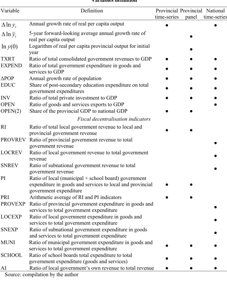
Table 2.2 Variables definition
Source: compilation by the author
Variable Definition Provincial
time-series Provincialpanel time-seriesNational
t
y
ln
∆
Annual growth rate of real per capita output ● ●t
y
ln
∆
5-year forward-looking average annual growth rate ofreal per capita output ●
)
0
(
ln y
Logarithm of real per capita provincial output for initialyear ●
TXRT Ratio of total consolidated government revenues to GDP ● ● ● EXPEND Ratio of total government expenditure in goods and
services to GDP ● ● ●
∆POP Annual growth rate of population ● ● ● EDUC Share of post-secondary education expenditure on total
government expenditures ● ● ● INV Ratio of total private investment to GDP ● ● ● OPEN Ratio of goods and services exports to GDP ● OPEN(2) Share of the provincial GDP to national GDP ● ●
Fiscal decentralisation indicators RI Ratio of total local government revenue to local and
provincial government revenue ● ● PROVREV Ratio of provincial government revenue to total
government revenue ●
LOCREV Ratio of local government revenue to total government
revenue ●
SNREV Ratio of subnational government revenue to total
government revenue ●
PI Ratio of local (municipal + school board) government expenditure in goods and services to local and provincial
government expenditure ● ● PRI Arithmetic average of RI and PI indicators ● ● PROVEXP Ratio of provincial government expenditure in goods and
services to total government expenditure ● LOCEXP Ratio of local government expenditure in goods and
services to total government expenditure ● SNEXP Ratio of subnational government expenditure in goods
and services to total government expenditure ● MUNI Ratio of municipal government expenditure in goods and
services to total government expenditure ● ● ● SCHOOL Ratio of school boards total expenditure to total
government expenditure (goods and services) ● ● ● AI Ratio of local government’s own revenue to total revenue ● ● ●
2.3 The data
Data were taken from Statistics Canada’s CANSIM II database. Table 2.2 lists the tables used from CANSIM II to retrieve the data necessary for this paper.
Table 2.3 CANSIM II Tables
Table number Table Title
Provincial data
510005 Estimates of Population, Canada, Provinces and Territories
3840001 Gross domestic product (GDP), Income-based, Provincial Accounts
3840002 Gross domestic product (GDP), expenditure-based, provincial economic accounts
3840004 Government sector revenue and expenditure, provincial economic accounts 3840015 Provincial Gross Domestic Product (GDP), Expenditure-based
3840022 Federal Government and Government Sector Revenue and Expenditure 3840023 Provincial Government Revenue and Expenditure
3840024 Local Government Revenue and Expenditure
4780001 Total Expenditure on Education, by Direct Source of Funds and Type of Education
4780010 School Board Revenues, by Direct Source of Funds 4780012 School Board Expenditures, by Economic Classification
National data
3800017 Gross Domestic Product (GDP), Expenditure-based 3800022 Sector Accounts, All Levels of Government
3800040 Gross Domestic Product (GDP), Expenditure-based
3850001 Consolidated Federal, Provincial, Territorial and Local Government Revenue and Expenditure, for Fiscal Year Ending March 31
Source: author
A few important remarks need to be made on the data involved in this research paper. First of all, due to their historical nature, it was necessary to compute observations for most provincial series from two different tables. Provincial GDP series were found for the 1961-1991 period in table 3840015 Provincial Gross Domestic Product (GDP), Expenditure-based and for the 1981-2004 period in the table 3840002 Gross domestic product (GDP), expenditure-based, provincial economic accounts. When divergences occurred between the two data sets, which we found was usually between 1 and 5%, we used the observations compiled in the latest of the two tables. Consolidated provincial budgetary series were also compiled from two different tables. Total government revenue
series, used to calculate the TXRT variable, a global measure of the tax burden of a provincial economy, were taken from tables 3840022 Federal Government and Government Sector Revenue and Expenditure and 3840004 Government sector revenue and expenditure, provincial economic accounts. Since all amounts were in nominal terms, we used provincial GDP in current dollars to calculate most ratios. Provincial nominal GDP series were found in table 3840015 for 1961-1991 and table 3840001 Gross domestic product (GDP), Income-based, Provincial Accounts for 1981-2004. The variable EXPEND, the spending equivalent of TXRT used in regressions with expenditure-type decentralization indicators, was compiled with national account series taken from tables 3840015 and 3840002. Similarly, the variable INV, the ratio of private investment in fixed capital and machines to GDP used data from the same national account series for both sub periods. To compute ∆POP, the annual growth rate of total population, we used single series since the data was accessible for 1954 to 2004. Finally for series on spending in post-secondary education by all levels of government used to compute EDUC, a proxy for human capital in each province, data was taken from table 4780001 Total Expenditure on Education, by Direct Source of Funds and Type of Education up to 1999, the last year data was compiled by Statistics Canada for this expenditure category. This constraint was one of the reason we used 4 lags on independent variables for our provincial regressions.
Data used for the decentralization indicators (RI, PI, MUNI, SCHOOL, PRI and AI) for local and provincial government expenditure had to be disaggregated between the two levels and were only accessible on CANSIM II up to 2002. Data on local government revenue and expenditure for 1961-1991 were taken from table 3840024 Local Government Revenue and Expenditure and table 3840004 for 1981-2004. Local government expenditure was divided between general spending and school board expenditure. This was done in order to capture the potentially different effects of these two categories. While we could suspect general local government spending to be positively correlated with growth, due to greater proximity to local needs and greater sensitivity to government competition, school board expenditure should be negatively correlated with growth due to the benefits of greater coordination and economies of scale.
This is in accordance with Oates’ 4 rules for decentralization. Municipal governments face a high level of heterogeneity in the public services they offer, therefore favouring more decentralization. Taxpayers may also benefit from increased competition between municipalities. On the other hand, we could suspect a relatively high homogeneity in people’s preferences for schools and important economies of scale in school systems. We will try to identify these effects in the subsequent section on our regressions analysis.
Another issue concerning school board revenue and expenditure had to be dealt with specifically for Newfoundland. We found that Statistics Canada did not compile local government budgetary data the same way it did for the rest of Canadian provinces. In Newfoundland’s case, the Total Revenue series (V503369) found in table 3840024 Local Government Revenue and Expenditure did not include for the 1961-1991 period school board revenue, while the corresponding series for 1981-2002, Local Government; Total Revenue (V689577) from table 3840004 did contain those amounts. The explanation is that school boards in Newfoundland are operated by religious organization and not by the government. The result was a near 14 point jump in local government revenue between 1980 and 1981. We therefore had to add to the older series Total Revenues (V1025855) from table 4780010 School Board Revenue, by Direct Source Funds. The same correction had to be made on the expenditure side since the 1961-1991 data did not contain school board expenditure, while the 1981-1991 series did contain it. Finally, our indicator of local government autonomy AI also had to be adjusted to take into account this change. Not only did we have to modify data on local government revenue, but we also had to add transfers from provincial government to school boards to transfers from provincial to local government.
A similar observation needs to be made for New Brunswick. The province underwent a reform of its education system in 1967 and with it, came the abolition of school boards.19 Consequently according to the data, local government revenue had a 60% drop from 1966 to 1967. The reason was school board revenue was no longer
compiled at the local level, but at the provincial level and this is why the provinces presents such a different decentralization profile than other provinces in Canada.
One final correction had to be made with provincial data. Observations on provincial government spending for goods and services from table 3840004 Government sector revenue and expenditure, provincial economic accounts for 1981-2002 has been compiled in CANSIM II with school board expenditure included. The older data for 1961-1991 did not include these amounts, so we found a very large gap between the two series. We made the correction by subtracting school board expenditure from provincial expenditure in the new series.
National data was much simpler to work with. Single series could be found for the whole period we were concerned with, except for data on education expenditure. Therefore, for most series no adjustments were needed in order to use the data directly from CANSIM II. As for education, the data was needed to compute the decentralization indicators MUNI, spending by municipal governments and SCHOOL, spending by school boards as well as EDUC, our proxy for human capital, measured by government spending on higher education as a share of total government spending. Data was accessible on these spending categories for 1954-2000 in table 4780001 Total Expenditure on Education, by Direct Source of Funds and Type of Education and for 1989-2004 in table 3850001 Consolidated Federal, Provincial, Territorial and Local Government Revenue and Expenditure, for Fiscal Year Ending March 31. We combined both series to have government spending on both higher education as well as school board expenditure for the whole 1961-2004 period. Finally, all independent variables were included in the regressions with a one-year lag except EDUC and INV, which were both included with 5-year lags, which provided us with the most significant regression results.
To end this section, we present in table 2.4 decentralization indicators for the 10 provinces calculated in various years to present each province’s profile and its evolution over time.
Table 2.4
Fiscal decentralization by province and indicators for selected years
Province Year RI PI MUNI SCHOOL PRI AI
NFD 1962 0.18 0.31 0.05 0.25 0.25 0.31 1972 0.21 0.46 0.08 0.38 0.34 0.18 1982 0.21 0.38 0.07 0.32 0.30 0.20 1992 0.19 0.39 0.12 0.27 0.29 0.25 2000 0.19 0.30 0.12 0.18 0.25 0.23 PEI 1962 0.19 0.42 0.03 0.38 0.31 0.50 1972 0.16 0.36 0.03 0.32 0.26 0.15 1982 0.16 0.4 0.09 0.31 0.28 0.14 1992 0.17 0.32 0.05 0.27 0.25 0.14 2000 0.17 0.3 0.08 0.21 0.24 0.20 NS 1962 0.31 0.51 0.10 0.42 0.41 0.66 1972 0.27 0.49 0.12 0.37 0.38 0.49 1982 0.28 0.45 0.15 0.30 0.37 0.35 1992 0.26 0.41 0.16 0.25 0.34 0.39 2000 0.21 0.39 0.18 0.22 0.30 0.48 NB 1962 0.31 0.51 0.13 0.38 0.41 0.60 1972 0.08 0.11 0.11 0.00 0.10 0.39 1982 0.10 0.10 0.10 0.00 0.10 0.47 1992 0.09 0.10 0.10 0.00 0.10 0.59 2000 0.08 0.10 0.10 0.00 0.09 0.72 QUE 1962 0.39 0.69 0.19 0.50 0.54 0.69 1972 0.32 0.59 0.16 0.43 0.46 0.49 1982 0.28 0.47 0.17 0.29 0.38 0.41 1992 0.27 0.41 0.18 0.23 0.34 0.5 2000 0.22 0.42 0.18 0.23 0.32 0.54 ONT 1962 0.46 0.73 0.29 0.44 0.60 0.60 1972 0.38 0.61 0.20 0.40 0.50 0.52 1982 0.36 0.61 0.26 0.35 0.49 0.54 1992 0.38 0.59 0.24 0.36 0.49 0.55 2000 0.31 0.57 0.25 0.32 0.44 0.58 MAN 1962 0.42 0.68 0.29 0.39 0.55 0.72 1972 0.32 0.53 0.16 0.37 0.43 0.56 1982 0.30 0.46 0.18 0.28 0.38 0.47 1992 0.26 0.44 0.16 0.28 0.35 0.47 2000 0.22 0.41 0.14 0.27 0.32 0.52 SASK 1962 0.37 0.68 0.28 0.40 0.53 0.66 1972 0.30 0.57 0.18 0.39 0.44 0.62 1982 0.28 0.44 0.17 0.27 0.36 0.53 1992 0.24 0.44 0.17 0.27 0.34 0.54 2000 0.20 0.41 0.18 0.23 0.31 0.67 ALTA 1962 0.45 0.65 0.18 0.47 0.55 0.59 1972 0.35 0.57 0.16 0.40 0.46 0.54 1982 0.26 0.47 0.19 0.28 0.37 0.5 1992 0.29 0.45 0.18 0.27 0.37 0.55 2000 0.21 0.44 0.18 0.26 0.33 0.46 BC 1962 0.38 0.60 0.19 0.41 0.49 0.62 1972 0.33 0.52 0.15 0.37 0.43 0.59 1982 0.28 0.44 0.17 0.27 0.36 0.49 1992 0.25 0.41 0.16 0.25 0.33 0.37 2000 0.20 0.38 0.17 0.21 0.29 0.46 Source: compilation from CANSIM II by the author
From the preceding table, we can see that Ontario stands out as being the most decentralized province in Canada. All decentralization indicators except AI, a measure of local government autonomy, rank highest for the most populated Canadian province. On the other hand, the least decentralized province as revealed by our indicators is Prince-Edward-Island. It is also the smallest and least populated province, which is somewhat not surprising to find. Finally, there seems to be a clear downward trend in decentralization in Canada according to all indicators. 2000 levels are on average 30% lower than 1962 levels. Following is a correlation matrix of our 6 provincial indicators.
Table 2.5
Correlation coefficients of fiscal decentralization indicators, 1961-2000
RI PI MUNI SCHOOL PRI AI
RI - - - - PI 0.815 - - - - - MUNI 0.167 0.310 - - - - SCHOOL 0.809 0.951 0.064 - - - PRI 0.899 0.982 0.273 0.943 - - AI 0.513 0.439 0.082 0.435 0.474 - Source: compilation from CANSIM II by the author
Chapter 3 – Empirical Results
Results for the provincial time-series regressions are found in Annex 2, we will provide here a summary of significant results. One important observation is the larger the province, the more explanatory power independent variables had in our regressions. A good measure of this explanatory power is adjusted R-square which has low values for some of the provinces. In particular, regressions for Prince-Edward-Island all yield negative values of this statistic. In fact, we do not find any significant variable in the 7 regressions. Table 3.1 gives a summary of significant results found in our provincial time-series regressions.
Table 3.1
Statistically significant regression results, provincial time-series 1965-2004
Source: compilation by the author
As we can see from the previous table, significant results can be found in 6 of the 10 provinces. From these results, it seems that decentralization has mostly contributed to provincial economic growth. Except for New Brunswick, which has a very high coefficient (in absolute terms) associated to the MUNI indicator, all the coefficient above indicate that the more revenue and expenditure were handled by local government Regression Indicator Coefficient Sign. level Max adj. R² Min adj. R²
NFD - - - 0.08 0.04 PEI - - - -0.02 -0.07 NS PI 0.29 5% 0.09 0.22 MUNI 0.69 10% - - SCHOOL 0.33 5% - - NB MUNI -1.46 10% -0.02 -0.10 QUE - - - 0.25 0.32 ONT SCHOOL 0.59 5% 0.20 0.30 MAN RI 0.79 10% 0.08 -0.01 PRI 0.47 10% - - SASK RI 1.13 5% 0.15 0.02 PI 0.57 5% - - MUNI 1.30 5% - - PRI 1.29 5% - - ALTA - - - 0.20 0.17 BC RI 0.70 5% 0.19 -0.05 PRI 0.88 1% - -
officials, the better was the economic performance. The effects of decentralization seems to have been relatively stronger in Saskatchewan, where an additional percentage point of municipal expenditure as a share of total government expenditure was associated with a 0.013 percentage point increase in the province GDP growth rate. Also, we did not obtain negative coefficient for the variable SCHOOL like we hypothesized. In all three cases where the variable had a significant coefficient, the value was positive. After running time-series regression for individual provinces, we compiled data in order to run panel regressions, first using observations for all 10 provinces and then only using the 6 largest provinces (excluding the smaller Atlantic provinces). Results for these two regressions are given in tables 3.2 and 3.3 below.
Table 3.2
Regression results for provincial panel data
Source: Statistics Canada (CANSIM II)
Dependant variable : 5-year forward-looking average per capita GDP growth rate
Indep. var. (1) (2) (3) (4) (5) (6) (7) PIB(0) 0.00 0.00 -0.02 -0.01 0.00 0.00 0.00 [-0.08] [-0.39] [-0.93] [-0.91] [-0.21] [-0.31] [-0.07] TXRT -0.26 - - - - -0.25 -0.26 [-2.42]** - - - - [-2.33]** [-2.49]** SPENDTOT - -0.25 -0.26 -0.26 -0.25 - - - [-2.32]** [-2.41]** [-2.46]** [-2.34]** - - RI 0.00 - - - [-0.08] - - - PI - 0.01 - - - - [0.64] - - - MUNI - - 0.08 0.07 - - - - - [1.07] [1.13] - - - SCHOOL - - 0.00 - 0.01 - - - - [-0.19] - [0.39] - - PRI - - - 0.01 - - - - [0.40] - AI - - - 0.00 - - - [-0.06] ∆POP -0.05 -0.04 0.13 0.11 -0.06 -0.04 -0.06 [-0.19] [-0.15] [0.40] [0.35] [-0.23] [-0.16] [-0.2] EDUC 0.04 0.06 0.08 0.08 0.05 0.06 0.04 [0.48] [0.75] [0.95] [0.98] [0.65] [0.67] [0.51] INV -0.02 -0.02 -0.04 -0.04 -0.02 -0.02 -0.02 [-0.41] [-0.57] [-0.85] [-0.84] [-0.48] [-0.51] [-0.39] OPEN -0.01 -0.01 -0.02 -0.02 -0.01 -0.01 -0.01 [-0.44] [-0.43] [-0.76] [-0.74] [-0.39] [-0.44] [-0.43] Time1 -0.01 -0.02 -0.03 -0.02 -0.01 -0.01 -0.01 [-0.64] [-0.73] [-1.10] [-1.08] [-0.65] [-0.70] [-0.53] Time2 -0.03 -0.04 -0.04 -0.04 -0.03 -0.03 -0.03 [-2.10]** [-2.22]** [-2.41]** [-2.44]** [-2.15]** [-2.19]** [-1.86]* Time3 0.01 0.01 0.01 0.01 0.01 0.01 0.01 [1.18] [1.04] [0.65] [0.69] [1.14] [1.07] [1.10] Time4 -0.02 -0.02 -0.02 -0.02 -0.02 -0.02 -0.02 [-1.84]* [-1.87]* [-2.05]** [-2.05]** [-1.83]* [-1.86]* [-1.80]* Time5 -0.03 -0.03 -0.03 -0.03 -0.03 -0.03 -0.03 [-3.35]*** [-3.30]*** [-3.42]*** [-3.48]*** [-3.27]*** [-3.32]*** [-3.34]*** Time6 -0.04 -0.04 -0.04 -0.04 -0.04 -0.04 -0.04 [-4.27]*** [-4.24]*** [-4.31]*** [-4.34]*** [-4.23]*** [-4.24]*** [-4.26]*** Time7 -0.01 -0.01 -0.01 -0.01 -0.01 -0.01 -0.01 [-1.10] [-1.16] [-1.30] [-1.29] [-1.12] [-1.15] [-1.11] CONS 0.15 0.17 0.28 0.27 0.15 0.17 0.15 [1.26] [1.52] [1.74]* [1.79]* [1.40] [1.44] [1.04] Adj. R-square 0.67 0.67 0.67 0.67 0.67 0.67 0.67 Hausman test 3.99 6.48 6.81 6.06 4.91 4.95 4.50 P-value 1.00 0.95 0.96 0.97 0.99 0.99 0.99 Obs. 80 80 80 80 80 80 80