Modelisation of perfluorocarbon emissions based on the alumina distribution and local current density in an aluminium electrolysis cell

A DISSERTATION PRESENTED TO THE

UNIVERSITY OF QUEBEC AT CHICOUTIMI IN PARTIAL FULFILLMENT OF THE REQUIREMENT FOR THE DOCTOR OF PHILOSOPHY IN ENGINEERING

BY LUKAS DION

MODELISATION OF PERFLUOROCARBON EMISSIONS BASED ON THE ALUMINA DISTRIBUTION AND LOCAL CURRENT DENSITY IN AN ALUMINIUM

ELECTROLYSIS CELL

RÉSUMÉ

L’industrie de l’aluminium est une importante productrice de GES à l’échelle nationale tant par ses émissions de dioxyde de carbone que par ses émissions de perfluorocarbures (PFC) qui émanent lors d’un événement néfaste communément appelé effet anodique (EA). Le projet de doctorat discuté dans le présent document a été mis en place pour accroître la compréhension des mécanismes qui entraînent des émissions de PFC de façon à faciliter leur quantification tout en minimisant les émissions totales.

Globalement, les émissions de PFC pour une usine sont actuellement quantifiées en utilisant des modèles linéaires qui nécessitent des indicateurs de performance mensuels. Ces méthodologies sont toutefois imprécises pour une faible fréquence d’EA et de nouveaux modèles sont désormais nécessaires pour assurer une quantification adéquate des émissions de PFC.

Au cours du projet, plusieurs campagnes industrielles de mesure d’émissions ont été réalisées pour associer une quantité de CF4 et de C2F6 spécifique à chacun des EA

respectifs détecté par le système de contrôle. En se basant sur plus de mille EA individuels mesurés, de nouveaux modèles ont pu être proposés et ceux-ci ont été comparés avec les modèles déjà existants établis. Le modèle considéré comme ayant le meilleur potentiel (simple et efficace) pour une utilisation à travers l’ensemble de l’industrie considère une évolution non linéaire de la quantité de PFC émise en fonction de la durée de polarisation mesurée pendant l’EA. Une validation basée sur les performances de sept usines a permis de confirmer une meilleure précision du modèle proposée. Toutefois, l’ampérage de l’usine à un impact considérable sur le rythme d’émission des PFC. Il a donc été nécessaire d’incorporer une seconde variable dans l’équation pour un meilleur degré de précision. Ainsi, le modèle générique développé permet de quantifier individuellement les émissions de PFC issues d’EA pour toutes les technologies utilisant des anodes précuites et ayant un ampérage inférieur à 440 kilo ampères.

Le deuxième volet du projet touche les effets anodiques à bas voltage (EABV) en mettant l’emphase sur les mécanismes entraînant leur génération. À partir de mesure de composition des gaz de cuves individuelles, un premier modèle publié a été mis en place permettant de quantifier les émissions de PFC issues d’EABV. Ce modèle a une précision de ±25% pour le 2/3 des cas observés. Une analyse de sensibilité performée sur ce modèle a permis de déterminer que l’écart-type de courant anodique individuel est le paramètre ayant la meilleure corrélation avec les émissions de PFC issues d’EABV. Il a également été possible de démontrer qu’un changement dans la méthode d’échantillonnage des gaz offrirait une meilleure représentativité du comportement de la cuve, ce qui est nécessaire pour atteindre une précision plus élevée de l’algorithme de prédiction des EABV.

Un modèle mathématique transitoire a été développé permettant de simuler l’évolution de la distribution locale d’alumine et la densité du courant dans une cuve d’électrolyse pour les 20 ensembles anodiques de la cuve. Il est donc possible d’évaluer l’homogénéité de la distribution du courant et de prédire si certains scénarios d’opération sont plus à risque de générer des PFC. Des mesures industrielles ont permis de confirmer une bonne corrélation entre le simulateur et la réalité, autant au niveau de l’évolution de la concentration d’alumine que pour la prédiction d’EABV.

Enfin, les connaissances acquises au cours du projet et la proximité du partenaire industriel ont permis la mise en place d’un algorithme de contrôle des cuves qui détecte la production de PFC dans la cuve et lance automatique un traitement correctif qui agit pour éliminer cette problématique. Cette action corrective a permis une réduction de plus de 50% de la fréquence des EA ainsi qu’une réduction de près de 50% de l’instabilité des cuves étudiées sans affecter de façon négative les autres indicateurs clés de performances.

SUMMARY

The aluminium industry is an important GHG producer due to its carbon dioxide emissions but also due to the perfluorocarbons (PFC) emissions emitted during a detrimental event known as anode effect (AE). The doctoral project presented in this thesis was realised to increase the understanding of the different mechanisms leading to the generation of PFC, in order to facilitate the quantification of PFC while facilitating a reduction of the total emissions.

Globally, a smelter’s PFC emissions are estimated using linear models based on monthly performance indicators. However, the precision of these methodologies is dependent on the total number of AE occurrence and new models are now necessary to assure adequate estimations of PFC emissions.

During this project, multiple measurement campaigns were performed to assign specific CF4 and C2F6 amounts for each respective AE detected by the control system.

Based on more than one thousand individual measurements, new models were proposed and compared to the already existing methodologies. The model considered with the best potential to be used widely across the industry, in terms of simplicity and efficiency, considers the PFC emission rate as a non-linear function of the polarised AE duration. Validation was performed based on data acquired in 7 different smelters to confirm an improved predictive efficiency. However, it also demonstrated that the line current has an important impact on the emission rate of PFC emissions. It was necessary to incorporate an additional variable into the equation to reach a higher level of precision. Finally, a generic model was developed with the ability to estimate the PFC emissions resulting from individual AE for cell technologies using prebaked anodes and line current higher than 440 kilo amperes.

The second aspect of the project is related to low voltage anode effect (LVAE) where a thorough study of the mechanism leading to their generation was performed. Based on gas composition measurements performed on individual cells, a first published model was established allowing quantification of PFC emissions resulting from LVAE. The measured accuracy of the model is ±25% for 2/3 of the studied scenarios. A sensitivity analysis was performed afterward on the model and the standard deviation among individual anode currents was found to be the variable having the best correlation with the presence of LVAE. It was also demonstrated that improvements in the gas extraction technique should lead to a better representativeness of the cell global condition, which is necessary in order to increase the predictive capability of the LVAE algorithm.

A transient mathematical model was developed to simulate the local alumina concentration and current density in an electrolysis cell for the 20 different anodic assemblies. Henceforth, it is possible to evaluate the homogeneity of the current distribution and predict if specific operation scenarios are more at risk to generate PFC

emissions. Industrial measurements confirmed that a good correlation exists between the simulator and the reality for both the evolution of the alumina distribution and the LVAE predictive capability.

Finally, the knowledge acquired during this project and the proximity of the industrial partner allowed the development of a control algorithm to detect PFC generation while automatically launching a corrective action to eliminate the threat. Usage of this preventive treatment allowed a reduction of more than 50% on the AE frequency and a reduction of almost 50% related to the cell instability without any negative impact on other key performance indicators.

REMERCIEMENTS

Au cours de mon cheminement académique, j’ai eu la chance de côtoyer un très grand nombre de personnes et je crois fortement que chacune d’entre elle m’ont influencé de façon positive. Ces quelques lignes visent à souligner les gens que je considère comme pierres angulaires de mon cheminement et sans qui, je n’aurais pas eu les mêmes succès.

En tout premier lieu, je désire remercier profondément mon directeur de recherche, Pr. László Kiss, non seulement pour le soutien constant que celui-ci m’a offert durant tout le projet, mais pour le partage de son enthousiasme contagieux qui a eu de nombreuses répercussions positives dans toutes les sphères de ma vie.

En second lieu, le support de mon codirecteur de recherche, Dr. Sándor Poncsák, a été très fortement apprécié au cours des trois dernières années. Son attitude professionnelle minutieuse a permis d’accroître considérablement la qualité de mes travaux scientifiques. Par ailleurs, je suis très reconnaissant pour ses rappels sur l’importance d’un bon équilibre entre le travail et les loisirs, de façon à demeurer en pleine forme mentalement, et ainsi performer à son plein potentiel.

Par la suite, je tiens à remercier mon superviseur en milieu pratique, M. Charles-Luc Lagacé, pour son soutien continu dans toutes les phases du projet, particulièrement lors de la phase initiale qui a permis de bien combiner plusieurs aspects fondamentaux avec les besoins industriels.

Il y a également plusieurs employés travaillant chez Aluminerie Alouette qui m’ont prêté main-forte à plusieurs reprises pour m’aider à réaliser mes expérimentations, assez souvent… hors du commun.

Parmi ces employés, une mention très spéciale à Guy Ladouceur, ainsi qu’un grand merci à toutes ces personnes formidables avec qui j’ai eu la chance de passer du temps : Marc Gagnon, François Laflamme, Patrick Coulombe, Nadia Morais, Julie Salesse, Stephan St-Laurent, Dominic Dubé, Antoine Godefroy, et bien d’autres que j’oublie…

Je remercie grandement le Dr. Jerry Marks pour son assistance technique, ainsi que pour m’avoir permis d’utiliser à plusieurs occasions un appareil de mesure de type FTIR chez Aluminerie Alouette. Sans cette contribution, il n’aurait pas été possible de réaliser un projet d’une telle ampleur.

J’en profite aussi pour remercier certains collaborateurs avec qui j’ai eu la chance de travailler sur de superbes projets. Ces collaborateurs sont James Evans, Simon Gaboury, Jerry Marks, Pernelle Nunez, David Wong et Alexey Spirin.

Bien entendu, la réalisation d’un tel projet en milieu industriel aurait été impossible sans le partenariat d’Aluminerie Alouette. Je tiens donc à mentionner que je suis

extrêmement reconnaissant de l’envergure du support que j’ai reçu, autant du côté technique que sur l’aspect financier. Le soutien financier de la part du CRNSG et du FRQNT, au moyen d’une bourse d’études BMP-Innovation est également grandement apprécié.

Par ailleurs, d’autres organisations m’ont également soutenu au moyen de bourses d’excellences, ou de bourse de soutien pour assister à des rencontres scientifiques. Je suis donc très reconnaissant auprès de la Fondation UQAC, de Rio Tinto, ainsi qu’auprès de la fondation TMS.

Enfin, je considère que l’ensemble de mes succès sont en grande partie fondés sur l’appui reçu de la part de mes parents, Gilles Dion et Michèle Savard qui sont une source perpétuelle d’encouragement et de motivation.

En tout dernier lieu, il m’aurait été impossible d’arriver au même point, après ces dix années d’études universitaires, sans le support de ma famille, de mes amis munchkineux, de mes deux chats, et surtout, sans le soutien de ma conjointe Karine Leblanc, avec qui j’ai traversé toutes les étapes importantes de ma vie.

TABLE OF CONTENT

Résumé ... III Summary ... V Remerciements ... VII Table of Content ... IX List of figures ... XIV List of tables ... XVIII

1. Chapter 1 Introduction ... 1 Introduction – Hall-Heroult process ... 2 1.1

Generation of Greenhouse Gases ... 3 1.1.1

Distinction between high voltage and low voltage anode effects ... 4 1.1.2

Goals of the thesis ... 6 1.2

Methodologies ... 7 1.3

Experimental work ... 7 1.3.1

Overview and Relationship Between the Different Chapters ... 11 1.4

References ... 12 1.5

2. Chapter 2 Quantification of perfluorocarbons emissions during high voltage anode effects using non-linear approach (based on data from a single smelter) ... 13

Summary ... 14 2.1

Introduction ... 14 2.2

State of the art... 16 2.3

Anode effect definition ... 16 2.3.1

Observations from previous publications ... 19 2.3.2

Standard Quantification Methodologies ... 20 2.3.3

Methodology ... 22 2.4

Experimental setup ... 22 2.4.1

Preparation of the data ... 23 2.4.2

Results and discussion (analysis on a single smelter’s performances) ... 27 2.5

Description of the different models to predict CF4 ... 29

2.5.1

Description of the different models to predict C2F6 emissions ... 36

2.5.2

Validation ... 40 2.5.3

The possible impact of the proposed models for the aluminium industry. ... 44 2.5.4

Conclusions ... 46 2.6

Additional content not presented in the original paper... 48 2.7

In-situ study on the traveling time of CF4 and C2F6 in the gas collection system ... 48

2.7.1

References ... 51 2.8

3. Chapter 3 New approach for quantification of perfluorocarbons resulting from high voltage anode effects (based on the data from multiple smelters) ... 54

Summary ... 55 3.1

Introduction ... 55 3.2

Anode effect mechanisms and quantification of emissions ... 56 3.3

Generation of perfluorocarbons caused by anode effects ... 56 3.3.1

Standard Quantification Methodology ... 58 3.3.2

Newly proposed quantification models ... 59 3.3.3

Collection of data: gas measurements ... 64 3.4

Results and Discussion ... 65 3.5

Efficiency of the different models to estimate individual HVAE emissions. ... 65 3.5.1

Efficiency of CF4 predictions ... 66

3.5.2

Efficiency of C2F6 Predictions ... 67

3.5.3

Comparison of the different models to account for HVAE emissions for smelters .... 3.5.4

... 71 Simplified approach using monthly averages and non-linear models ... 73 3.5.5

Conclusions ... 75 3.5.6

Additional content not presented in the original paper... 77 3.6

Development of a non-linear PAED prediction model for quantification of CF4 and

3.6.1

C2F6 emissions for cells with different line currents. ... 77

Performances of these generic models ... 84 3.6.2

Discussion of the results ... 87 3.6.3

References ... 88 3.7

4. Chapter 4 Prediction of low voltage tetrafluoromethane emissions based on the operating conditions of an aluminium electrolysis cell ... 89

Summary ... 90 4.1

Introduction ... 90 4.2

State of the Art ... 91 4.3

Experimental Setup ... 95 4.4

Development of the Predictive Algorithm ... 96 4.5

List of indicators ... 97 4.5.1

Description of the algorithm strategy ... 98 4.5.2

Results and discussion ... 100 4.6

Validation of the algorithm ... 100 4.6.1

Sensitivity analysis: individual effect of the indicators on the low voltage emissions 4.6.2 of CF4 ... 104 Conclusions ... 108 4.7 References ... 110 4.8

5. Chapter 5 Influence of hooding conditions on gas composition at the duct end of an electrolysis cell ... 112 Summary ... 113 5.1 Introduction ... 113 5.2 Experimental Setup ... 114 5.3

Cell and equipment specifications ... 114 5.3.1 Test methodology ... 116 5.3.2 Tracer gas ... 118 5.3.3 Additional measurements ... 121 5.3.4

Results and Discussion ... 122 5.4

Elements to consider to correctly interpret the results ... 122 5.4.1

Influence of the Tracer Gas Injection Point ... 124 5.4.2

Influence of the hooding conditions ... 127 5.4.3

Other Results of Interest ... 131 5.4.4

Conclusions ... 133 5.5

Additional content not presented in the original article ... 134 5.6

Proposition of a new sampling methodology ... 134 5.6.1 Experimental setup ... 135 5.6.2 Experimental results ... 137 5.6.3 References ... 138 5.7

6. Chapter 6 Simulator of non-homogeneous alumina and current distribution in an aluminium electrolysis cell to predict low voltage anode effects ... 139

Summary ... 140 6.1

Introduction ... 140 6.2

Generation of PFC During High Voltage and Low Voltage Anode Effects ... 142 6.3

Development of the Simulator ... 144 6.4

Input data, initial conditions ... 146 6.4.1

Alumina distribution ... 147 6.4.2

Electrical Current Distribution Module (Module 5) ... 157 6.4.3

Risk of low voltage anode effects (Module 7) ... 162 6.4.4

Validation of the simulator ... 163 6.5

Experimental setup ... 163 6.5.1

Validation of the Cell Voltage ... 166 6.5.2

Validation of the alumina distribution ... 167 6.5.3

Validation of the standard deviation among individual anode currents and validation 6.5.4

of PFC emissions ... 170 Further Improvements and Potential of the Simulator ... 172 6.6

Using the simulator to improve the electrolysis cell process ... 173 6.6.1

Conclusion ... 179 6.7

References ... 182 6.8

7. Chapter 7 Preventive treatment of anode effects using on-line individual anode current monitoring ... 184

Summary ... 185 7.1

Introduction ... 185 7.2

Early detection of the anode effects ... 186 7.3

Limit of detection of the current technology ... 186 7.3.1

Variations of individual anode currents during LVAE. ... 188 7.3.2

Development of the detection algorithm ... 189 7.3.3

Establishment of the Preventive AE Treatment ... 191 7.4

Preventive AE Treatment Parameters ... 192 7.4.1

Efficiency of AE Treatments to Unblock Feeder Holes ... 194 7.4.2

Key Performance Indicators of Cells With Automatic AE Treatment ... 198 7.5

Conclusion ... 202 7.6

References ... 204 7.7

8. Chapter 8 Conclusions and Recommendations ... 205 Conclusions ... 206 8.1

List of Innovative Realisations Performed During this Project. ... 210 8.1.1

Suggestions for Future Developments... 211 8.2

Estimation of HVAE Emissions. ... 211 8.2.1

Estimation of LVAE Emissions. ... 211 8.2.2

Simulator of Alumina and Current Distribution. ... 212 8.2.3

APPENDIX A – Reference spectra used during FTIR analysis ... 213 APPENDIX B – List of publications ... 218 APPENDIX C – Inputs and outputs of the different modules of the alumina and current

distribution simulator ... 220 APPENDIX D – Additional discussions ... 225

LIST OF FIGURES

Figure 1-1: Schematic of an aluminium electrolysis cell and its main components. [1] ... 2

Figure 1-2 : Illustration of an FTIR spectrometer main components [4]... 8

Figure 1-3 : Example of spectrum recomposition using a mixture of different gas reference. [4] ... 9

Figure 1-4 : Increase of the absorbance of CF4 with respect to the gas concentration. ... 10

Figure 2-1: Typical behavior of the cell voltage during an anode effect. ... 19

Figure 2-2: Decomposition of the CF4 concentration for overlapping HVAE. ... 26

Figure 2-3: Validation of the decomposition procedure. ... 27

Figure 2-4: Relative distribution of the polarized anode effect duration for the data considered. . 28

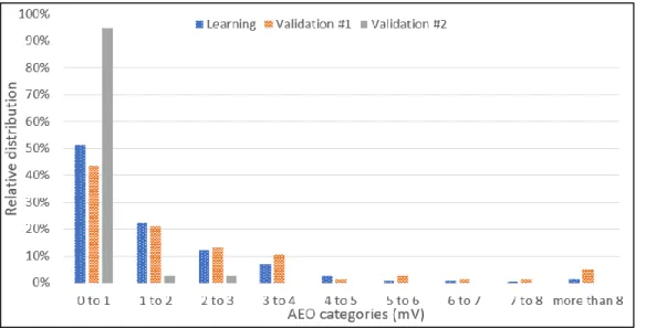
Figure 2-5: Relative distribution of the anode effect overvoltage for the data considered... 29

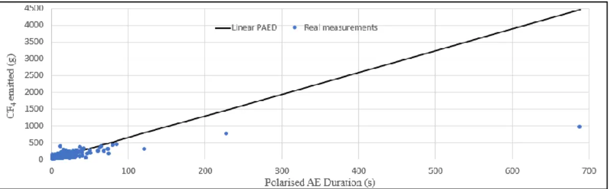
Figure 2-6: Linear PAED model in comparison to the real measured CF4 concentration from the learning group. ... 30

Figure 2-7: Linear AEO model in comparison to the real measured CF4 concentration from the learning group. ... 30

Figure 2-8: Non-linear PAED predictive model in comparison to subsidiary groups averaged CF4 emissions. ... 31

Figure 2-9: Non-linear AEO predictive model in comparison to subsidiary groups averaged CF4 emissions. ... 33

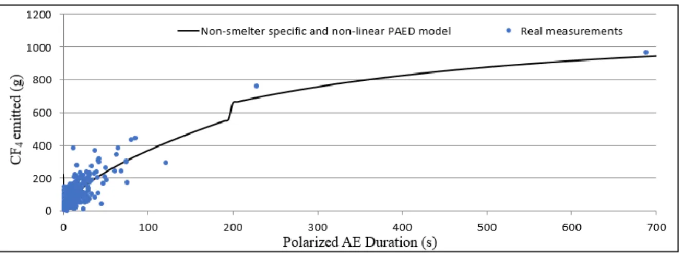
Figure 2-10: Non-smelter specific PAED non-linear model compared to real measurements from the learning group. ... 35

Figure 2-11: Cross-effect of PAED and MPV on the predicted emissions of CF4 using an MVA model. ... 36

Figure 2-12: C2F6 to CF4 ratio model in comparison to the real measurements. ... 37

Figure 2-13: Non-linear PAED model to represent C2F6 emissions along with average emissions from subsidiary groups. ... 38

Figure 2-14: Linear AED model to estimate C2F6 emissions along with the average results from subsidiary groups. ... 39

Figure 2-15: Cross-effect of PAED and MPV on the predicted emissions of C2F6 using an MVA model. ... 40

Figure 2-16: Overall errors and normalized squared residuals for predictive models regarding CF4 emissions. ... 41

Figure 2-17: Overall errors and normalized squared residues for predictive models regarding C2F6 emissions ... 42

Figure 2-18: Illustration of the gas travel course with injection points (blue stars). ... 49

Figure 2-19: Example of calculation of the travel time for each gas. ... 50

Figure 2-20: Different traveling time of the CF4 and C2F6 for injection point #2 and #3. ... 51

Figure 3-1:Illustration of the single range non-linear PAED model and its respective measurements. ... 62

Figure 3-2: Overall error (a) and squared errors (b) of the four predictive CF4 models for seven smelters. ... 66

Figure 3-3: Overall error (a) and squared errors (b) of the three predictive C2F6 models for five smelters. ... 68

Figure 3-4: Non-linear impact of the line current on PFC emission rate for HVAE with similar PAED. ... 70

Figure 3-5 : Estimated emissions of CF4 for 5 months of historical data for 6 different smelters

and the total average. ... 72

Figure 3-6 : Estimated emissions of C2F6 for 5 months of historical data for 6 different smelters and the total average. ... 73

Figure 3-7 :Comparison between the proposed methodologies and simplified “monthly” methodologies. ... 74

Figure 3-8: CF4 emission rate based on PAED for groups of smelters with different daily metal production. (A < B < C< D) ... 78

Figure 3-9: K1 and K2 behavior with respect to daily metal production to estimate CF4 emission rate. ... 79

Figure 3-10: Behavior of the K1 and K2 coefficient with respect to daily metal production to estimate C2F6 emission rate. ... 81

Figure 3-11: Surface graphs of the emission rate of CF4 for different daily metal production and polarized anode effect duration. ... 82

Figure 3-12: Surface graphs of the emission rate of C2F6 for different daily metal production and polarized anode effect duration. ... 83

Figure 3-13: Evolution of the C2F6/CF4 ratio based on the polarized anode effect duration and daily metal production for individual HVAE predictions. ... 84

Figure 3-14: Overall error (a) and squared errors (b) of the proposed model (PAED-DMP-Model) in comparison to the best performing model previously investigated (1R-NL-PAED) for CF4 predictions. ... 85

Figure 3-15: Overall error (a) and squared errors (b) of the proposed model (PAED-DMP-C2F6) in comparison to the best performing model previously investigated (C2F6-NL-PAED) for C2F6 predictions. ... 86

Figure 4-1: Illustration of the predictive algorithm strategy. ... 99

Figure 4-2: a) Percentages of correct and incorrect predictions after Step #1. b) Percentages of correct predictions along with the different offsets in incorrect predictions after Step #2. ... 101

Figure 4-3:Comparison between predicted CF4 concentrations (filled circles) and measured concentration (open circles). ... 102

Figure 4-4: Radar chart illustrating the absolute value of the error percentages for all 15 scenarios. ... 103

Figure 4-5: Influence level of each indicator on the frequency of predictions of CF4 based on a full-factorial design sensitivity analysis. The vertical line represents the measured threshold value for each variable. ... 106

Figure 5-1: Sketch of the gas collection within the test. ... 115

Figure 5-2: Top view of the cell showing all seven scenarios investigated. ... 118

Figure 5-3: Injection of the tracer gas during test #A11-TH. ... 119

Figure 5-4: Repeatability of individual balloons fill-up. ... 120

Figure 5-5: Example of a test sequence with the presence of LVAE emissions. ... 121

Figure 5-6: Superposition of two sections of the duct end. ... 124

Figure 5-7: Average mass of CF4 detected for all scenarios investigated. ... 125 Figure 5-8: Influence of hooding conditions during routine operations. (TD = Tapping doors open / A11, A15 and A20 represent hoods opened similar to an anode change of each

respective anode number / dashed line represents the reference average under perfect

hooding conditions). ... 128

Figure 5-9: Carbon monoxide emissions under different hooding conditions. ... 130

Figure 5-10: Possible contamination test coming from an adjacent cell. ... 132

Figure 5-11: Schematic of the new gas sampling methodology with 5 sampling probes ... 135

Figure 5-12: New and improved gas collection methodology ... 136

Figure 5-13: Flowmeters for the five sampling probes during testing. ... 136

Figure 5-14: Difference in accuracy between the original and the improved sampling methods. (Horizontal lines represent the inserted mass of CF4) ... 137

Figure 6-1: Sequential structure of the algorithms used in the simulator ... 146

Figure 6-2: Anodic assemblies, alumina feeders’ positions and alumina exchange between the different zones. ... 147

Figure 6-3: Illustration of the feeding sequence during a change in the feeding cycle. ... 149

Figure 6-4: Theoretical scenario used to determine the appropriate transport coefficient. ... 153

Figure 6-5: Impact of the diffusion on the alumina concentration of the different zones for a theoretical scenario with Deq= 3.7 m2/s. 10 zones are represented by a different curve. ... 153

Figure 6-6: Exchange between the different volumes based on the work of Thomas Hofer [21]. 155 Figure 6-7: Various elements considered as part of the electrical network. ... 158

Figure 6-8: Effect of the average alumina concentration in a cell on its pseudo-resistance. ... 162

Figure 6-9: Extraction points (stars) for bath samples during the test. Stars with the same colors represent areas where the bath was sampled simultaneously. ... 165

Figure 6-10:Comparison of the cell voltage between the simulator (dashed line) and real measurements (continuous line) (a) during different feeding cycles (b). ... 167

Figure 6-11: Comparison of the simulated alumina concentration history and real measurements. Figure a) to d) illustrates the results for scenario 1 to 4 respectively, with the initial hypotheses. Figure e) to h) illustrates the results for scenario 1 to 4 respectively after correction of the bath velocity. ... 169

Figure 6-12: Evolution of the simulated and measured standard deviation among individual anode currents during the four different validation scenarios, a) to d) respectively, along with the measured CF4 concentration. ... 171

Figure 6-13: Current distribution in the cell for similar anode conditions and different ACD. ... 174

Figure 6-14: Current distribution in the cell for different anode conditions and different ACD. . 175

Figure 6-15: Alumina concentration of the different regions at the end during the transition from underfeeding to overfeeding. ... 177

Figure 6-16: Impact of stopping a feeder after an important addition of parasite alumina. ... 178

Figure 7-1 : Individual anode currents and CF4 concentration from a single electrolysis cell during LVAE. ... 189

Figure 7-2 : Illustration of a cell behavior leading to preventive AE treatment. Upstream side. (Stars represent maximum current values reached for each individual anode during the short period.) ... 190

Figure 7-3 : Illustration of three different preventive anode effect treatment procedures. ... 195

Figure 7-4 : Illustration of a feeder before and after a preventive AE treatment. A) Blocked feeder. B) Unblocked feeder after a successful treatment... 196

Figure 7-5 : Performance indicators related to anode effects for the four periods of testing. ... 201

Figure A-1: CF4 reference spectra used during FTIR analysis ... 212

Figure A-2: C2F6 reference spectra used during FTIR analysis. ... 213

Figure A-3: SF6 reference spectra used during FTIR analysis. ... 213

Figure A-4: CO2 reference spectra used during FTIR analysis. ... 214

Figure A-5: CO reference spectra used during FTIR analysis. ... 215

Figure D-1: CF4 concentration of the dataset used in Chapter 4. ... 227

Figure D-2: Illustration of the bath flow reproduced from the thesis of Thomas Hofer, page 54. 230 Figure D-3: Linear regression between the simulated and measured alumina concentration for a) the initial hypotheses and b) the corrected bath velocity. ... 231

LIST OF TABLES

Table I: List of chemical compounds... XIX Table II: List of abbreviations ... XX Table III: List of symbols used in the different equations ... XXI Table IV. Overview of possible correlations between cell variables or specific events in the cell with low voltage emissions of PFC ... 93 Table V: Different dissolution coefficients estimated from published literature. ... 151 Table VI: Information related to the validation scenarios investigated. ... 164 Table VII : Success rates and the difference in bath levels for the tested preventive AE treatments. ... 197 Table VIII : Details on the four periods selected for testing the preventive AE treatments. 199 Table IX : Comparison between the test group and reference cells over four periods. ... 200

Table I: List of chemical compounds

Chemical formula Name

Al Aluminium

Al2O3

Aluminium oxide (Alumina) AlF3 Aluminium Fluoride

C Carbon

C2F6 Hexafluoroethane CaF2 Calcium Fluoride

CF4 Tetrafluoromethane

CO Carbon Monoxide

CO2 Carbon Dioxide

COF2 Carbonyl Fluoride

H2O Water

HF Hydrogen Fluoride

Na3AlF6 Cryolithe

NaF Sodium Fluoride SF6 Sulfur hexafluoroethane

Table II: List of abbreviations

Abbreviation Name

(diss) Chemical compound under dissolved form (g) Chemical compound under gas form

(l) Chemical compound under liquid form (s) Chemical compound under solid form ACD Anode-cathode distance (Interpolar distance)

AE Anode effect

AED Anode effect duration

AEO Anode effect Overvoltage

AETD Anode effect treatment duration (same thing as AED)

ANN Artificial neural network

AP40LE Specific type of cell technology: AP40 low energy

CE Current efficiency

CFD Computational fluid dynamics

CFx Family of PFC gas such as CF4, C2F6, C3F8 etc. FTIR Fourier-transform infrared spectrometer

GHG Greenhouse Gases

GTC Gas treatment center

HVAE High voltage anode effect

Hz Hertz

IAI International Aluminium Institute IPCC Intergovernmental Panel on Climate Change

kA Kilo ampere

LPM Liters per minute

LVAE Low voltage anode effect

m Meters

MHD Magneto-hydrodynamics

mm Millimeters

MPV Maximum polarisation voltage

mV Milivolts

MVA Multivariate analysis

PAED Polarized anode effect duration

PFC Perfluorocarbons

ppb Parts per billion

ppm Parts per million

Table III: List of symbols used in the different equations

Symbol Definition Units

Latin symbols

A Area of alumina exposed to bath m2 A

Cross-section area of an electrical

conductor m2

Abath Area of bath under an anode m

2

AEM Anode effect minutes per cells, per day

AE-Mins/cell-day Aij Contact area between two volumes m2

AOE Anode effect overvoltage mV

BR Bath ratio -

C Concentration of alumina in bath kg/m3 CCONS Daily carbon consumption m/day

CE Current efficiency %

CEi Respective current efficiency %

Cs

Concentration at saturation of alumina in

bath kg/m3 or % wt.

Deq Equivalent diffusivity m

2_/s

DMP Daily metal production (same as MP) tons

E0 Decomposition potential Volts

EC2F6 Total emissions of C2F6 kg

ECF4 Total emissions of CF4 kg

F Faraday's constant C/mol

F

Factor used to represent the effect of

bubbles under an anode -

FC2F6/CF4

Mass ratio between CF4 and C2F6

emissions used to estimate C2F6

emissions -

Ii

Respective amperage within an anodic

assembly A

K Kinetic of a reaction -

K1

Parameter used in the HVAE prediction power-law

g CF4 / tons Al / AE mins K2

Parameter used in the HVAE prediction

power-law -

Km Dissolution coefficient m/s

L

Length between the center of two

volumes m

L Length of an electrical conductor m LC Length of carbon on the anode m

LINI Initial carbon height of an anode m

LROD

Length of the aluminium rod of an anodic

assembly m

LTOT

Constant length from anodic beam to the

bottom of anodic assembly m

M Molar mass g/mol

mi Respective alumina consumption g

mij mass transfer rate between two volumes kg/s

MP Metal production for 24 hours tons

n Specific ratio -

N

Number of days since the anode is in the

cell days

OVC

Emission factor to estimate CF4 based on anode effect overvoltage

(kg CF4 / tonne

Al)/mV

R Resistance Ω

Rbath Resistance of the electrolyte Ω

SCF4

Emission factor to estimate CF4 emissions

based on the polarized anode effect duration (kg CF4/tonne Al)/(AE-mins/cell-day) T Bath temperature K or ˚C w Cell width m x

Dimensionless time during two simultaneous HVAE (0 = beginning and 1

= end) -

z Valency number of ions -

Mathematical symbols

∆C

Concentration gradient between two

volumes kg/m3

∆t Timestep s

∆x

Spatial distance between two volumes in

the simulator m

dm/dt dissolution rate of the alumina kg/s

Γ(x) Gamma function -

Greek symbols

α

Variable parameter used in the beta

α

Coefficient used in the calculation of the

saturation point of the alumina - β

Variable parameter used in the beta

function -

β

Coefficient used in the calculation of the

saturation point of the alumina -

ρ Electrical resistivity Ω m

ρbath Electrical resistivity of the bath Ω m

1. CHAPTER 1

INTRODUCTION

Introduction – Hall-Heroult process

1.1

Industrial aluminium production debuted in 1889, when Charles M. Hall and Paul Heroult developed, parallel to each other, a process to produce aluminium by electrolysis of the aluminium oxide using a cryolite-based solvent. This process, commonly known as the Hall-Heroult process has evolved over the century and is still widely used worldwide and considered the most practical way to obtain aluminium on an industrial scale.

Nowadays, electrolysis of the alumina is performed in large reduction cells (Figure 1-1) with a significant number of carbon anodes in parallel. An electrical current of high intensity passes through electrical conductors and these anodes to reach the cryolite-based electrolytic bath. A small concentration (typically 1 to 6%) of alumina is dissolved in the bath where the aluminium atoms will dissociate from the oxygen under the passage of a forced current through the electrolyte.

In most recent smelters, the alumina is routed automatically to the electrolysis cells structure, and then distributed to the bath periodically using point feeders located at specific points in the cell. The number of feeders will be dependent on the cell technology, which differs in size in order to accommodate for increasing line current. The cell technology considered in this project was operating with a total of four point feeders.

The composition of the electrolyte and the quality of the raw products (AlF3, Al2O3,

carbon anode, etc.) are very important to assure the consistency of the process, to maximize the production of aluminium and to reduce the occurrence of detrimental events such as anode effects. With increasing cell size and amperage, it has become a challenge to maintain homogeneity of the bath composition. For this reason, mathematical models developed to understand and predict the cell’s behavior became an essential element to improve the electrolysis process.

Finally, even after more than a century of operation using this process, there is still uncertainty regarding some of the dynamics of most of the reactions occurring during aluminium electrolysis. Some extensive studies are henceforth necessary to keep improving the general understanding of this process, more importantly regarding the generation rate of some gas products which have an important effect on the environment and climate change.

Generation of Greenhouse Gases 1.1.1

The aluminium industry is one of the most important anthropogenic producers of greenhouse gases (GHG), particularly because it uses carbon anodes1 which react with the

1 _{Cell technologies using inert anodes do not face these challenges. However, inert anodes have not yet}

oxygen from the alumina to produce carbon dioxide. Reaction 1-1 is inherent to the production of aluminium; therefore, the carbon dioxide emissions will be directly proportional to the annual aluminium production. Based on the mass balance of the process, more than 1.2 tons of CO2 is anticipated per tons of aluminium, with additional CO2

expected from carbon oxidation itself.

2 𝐴𝑙2𝑂3(𝑑𝑖𝑠𝑠)+ 3 𝐶(𝑠)→ 4 𝐴𝑙(𝑙)+ 3 𝐶𝑂_2(𝑔) (1-1)

Additionally, a second category of GHG is also produced by the aluminium industry: the perfluorocarbons (PFC). Tetrafluoromethane (CF4) and hexafluoroethane

(C2F6) are emitted during a detrimental event known as anode effect. This kind of incident

occurs when the alumina concentration in the bath becomes insufficient to support the passage of the electrical current. Under such circumstances, the electrolysis bath dissociates via reactions 1-2 and 1-3, and PFC gas is produced.

4 𝑁𝑎3𝐴𝑙𝐹_6(𝑙)+ 3 𝐶(𝑠)→ 4 𝐴𝑙(𝑙)+ 3 𝐶𝐹_4(𝑔)+ 12 𝑁𝑎𝐹(𝑑𝑖𝑠𝑠) (1-2) 2 𝑁𝑎3𝐴𝑙𝐹_6(𝑙)+ 2 𝐶(𝑠)→ 2 𝐴𝑙(𝑙)+ 𝐶2𝐹_6(𝑔)+ 6 𝑁𝑎𝐹(𝑑𝑖𝑠𝑠) (1-3)

Distinction between high voltage and low voltage anode effects 1.1.2

Anode effects may occur in the cell under different set of conditions based on the alumina feeding strategy and the size and bath volume of electrolysis cell. Within the industry, the common definition of an anode effect considers that the cell voltage needs to reach a specific threshold for a specific duration in order to be considered in anode effect. This trigger value is typically set to 8 volts, and the typical duration is 3 seconds [2]. Most recently, this type of event is referred to as high voltage anode effect (HVAE).

PFC emissions have also been observed in cases where the cell voltage did not reach the specific threshold of detection necessary for the cell control system to identify this event. Due to its small impact on the cell voltage, this type of emission is referred to as low voltage anode effect (LVAE). Even though the mechanism leading to the generation of PFC under LVAE is believed to be similar to HVAE emissions, the composition of the gas emitted appear to be mainly composed of CF4 and only little traces of C2F6 have been

observed under industrial LVAE conditions. This phenomenon has been explained by the alternative reaction 1-4 that necessitates a lower voltage of reaction and produces COF2

which reacts rapidly to form CF4 subsequently via equation 1-5.

2 𝐴𝑙𝐹3(𝑑𝑖𝑠𝑠)+ 𝐴𝑙2𝑂_{3(𝑑𝑖𝑠𝑠)}+ 3 𝐶(𝑠)→ 4 𝐴𝑙(𝑙)+ 3 𝐶𝑂𝐹_2(𝑔) E0 _{= -1.88V (1-4)} 2 𝐶𝑂𝐹_2(𝑔)+ 𝐶(𝑠)→ 2𝐶𝑂(𝑔)+ 𝐶𝐹_4(𝑔) K= 94.8 (1-5)

Wong et al. [3] characterized LVAE as 2 different categories:

 Non-propagating LVAE emissions: PFC emissions without impact on the cell voltage and occurring under a small number of anodes. This type of emission can last for several hours and remain undetected.

 Propagating LVAE emissions: PFC emissions having a small influence on the cell voltage, without reaching the detection threshold. This phenomenon affects a large number of anodes and can last a few minutes.

Whether or not a LVAE will propagate is dependent on the alumina distribution homogeneity in the cell. When generated, PFCs will wet the anode surface and reduce the current going through this specific anode. The current will be redirected to adjacent anodes which will increase their current density. If the alumina concentration is insufficient to handle the passage of these additional electric charges, it will eventually lead to a generation of PFC emissions under that adjacent anode. Under normal operation,

propagation of LVAE will only stop if the alumina distribution increases locally due to metal reoxydation or additional alumina feeding. If it doesn’t occur, the cell will eventually reach the HVAE state.

Even though both types of LVAE emissions have been observed in the scope of this project, references to LVAE in this thesis will always refer to both categories without any specific distinction.

Goals of the thesis

1.2

This project was designed to fundamentally understand the mechanisms leading to all types of PFC emissions (HVAE and LVAE). Moreover, the acquired knowledge should lead to the development of tools that would benefit the electrolysis process in order to reduce their carbon footprint, while offering improvements in terms of metal production. Hence the goals can be resumed as:

Main objective of the thesis

Being able to identify the key factors influencing the PFC generation rate in order to quantify or predict those emissions

for specific operation scenarios.

In order to achieve this main objective, the project was subdivided into three different parts. Moreover, each of the elements listed below are beneficial for the progress of science and well within the scope of a doctorate thesis:

1. Developing an improved methodology to quantify the PFC emission rate of cells during high voltage anode effect.

a. Determine the optimal way to predict, or detect the occurrence of LVAE in an electrolysis cell.

b. Develop a model to quantify LVAE resulting from process deviations occurring during aluminium electrolysis.

3. Developing a non-homogenous simulator to reproduce the cell behavior in terms of alumina and current distribution in order to predict PFC emissions within an electrolysis cell.

Methodologies

1.3

Experimental work 1.3.1

The project is realized in an industrial context. Thus, different kinds of measurements were necessary in order to acquire a satisfying amount of data to perform a successful analysis. The basics of these measurement techniques are presented in the following sections.

1.3.1.1 Gas Measurements

Analysis of the gas composition was performed under two different sets of conditions: individual cell gas composition monitoring and gas treatment center (GTC) gas composition monitoring. These sets of conditions are affected by the extraction point of the gas. However, in both cases the composition of the gas was determined using a Fourier-Transformed Infrared spectrometer (FTIR). FTIR spectrometry uses a calibrated infrared energy source generally emitting in a specific spectrum within the wave numbers range of 900 to 4000 cm-1. Under such circumstances, the energy emitted crosses the analysis chamber filled with the unknown compound; in this case, the gas extracted from the electrolysis cells.

An essential part of the FTIR is the interferometer, which is composed of a moving mirror illustrated on Figure 1-2, creating a phase shift in the emitted signal. Henceforth, the

detected signal is known as an interferogram which is directly dependent on the position of the moving mirror at a known time step minus the energy absorbed within the sample chamber.

Figure 1-2 : Illustration of an FTIR spectrometer main components [4].

Using Fourier analysis, it is possible to recompose the original spectrum across the entire wave numbers range within a single analysis taking only a fraction of second. This quick response time makes FTIR analysis an ideal technique to continuously analyze the fluctuating emissions of an aluminium electrolysis cell. Moreover, the precision of the measured spectrum can be significantly increased by performing the analysis multiple times

in a row, thus reducing the effect of the noise. The analyzed IR spectrum is then compared to the databank of gas reference in order to find the best correlation gas composition as shown in Figure 1-3.

Figure 1-3 : Example of spectrum recomposition using a mixture of different gas reference. [4]

The concentration of a gas will have a non-linear influence on the IR absorbance of the compound, thus it is important to have specific reference spectra in an order of magnitude similar to the expected emissions to assure representativeness of the results and to avoid extrapolation. The effect of an increasing CF4 concentration on the absorbance is

illustrated on Figure 1-4, for the primary absorption peak. Additional details on the reference spectra for various gases studied within the scope of this project are available in Appendix A.

Figure 1-4 : Increase of the absorbance of CF4 with respect to the gas concentration.

1.3.1.2 Electrolysis cell data acquisition

During normal operation of an electrolysis cells, the voltage is closely monitored continuously by the control system. Hence, no particular manipulation was necessary to acquire this information. Moreover, during HVAE conditions, the control system will automatically monitor the duration of the anode effect, and the energy released based on the evolution of the cell voltage in that time period. Finally, data on the alumina feedings of the cell were also recorded using the control system in order to determine their corresponding feeding cycles during the studied periods.

Even if this information is strongly relevant for the project, it only offers data on the global cell performance and cannot give details on the cell homogeneity. To accurately detect inhomogeneity in the alumina concentration, specific cells were selected when

performing tests on individual cells. These electrolysis cells were equipped with an on-line and continuous individual anode current monitoring system provided by Wireless Industrial Technologies [5]. This technology uses Hall effect sensors adjacent to the anode rods to measure the magnetic field, thus giving a clear indication of the anode current passing through that anode. Data was acquired with a 1 Hz frequency, which is sufficient to detect variation in the bath’s alumina concentration as demonstrated in a paper by Dion et al [6].

Overview and Relationship Between the Different

1.4

Chapters

As described in the previous sections, the goals of this thesis were covering three specific topics: Study of HVAE (1) and LVAE emissions (2), and development of an alumina and current distribution simulator (3). In order to demonstrate the magnitude of the work performed during this project, six chapters will be presented in this thesis covering the content of the work. This thesis is designed as a collection of articles which were all published prior to the final submission of this thesis. To avoid substantial changes to the originally published text from these articles, some additional discussions are provided in Appendix D.

In chapter 2, the quantification methods related to HVAE estimations are investigated. The inaccuracies of the actual methodologies are presented, and solutions are proposed to increase the predictive ability of PFC estimating models. On the other hand, chapter 3 investigates which type of non-linear models could be the most appropriate to be used across the entire aluminium industry.

Chapter 4 discusses the development and validation phases of the first published model with the ability to quantify PFC emissions resulting from LVAE. However, during the analysis of the results, some uncertainties related to the representativeness of the extracted gas were raised and these issues are discussed and evaluated in chapter 5.

Chapter 6 present the alumina and current distribution simulator, which indirectly connects all the themes of the thesis together. The development of the simulator, as well as the integration of a LVAE PFC estimation model are presented and discussed. In parallel, efficient ways to use this simulator to improve the industrial process are also presented.

Finally, in Chapter 7, industrial improvements resulting from the work performed in this thesis are presented, leading to a reduction of the HVAE frequency and overvoltage, as well as increased cell stability.

References

1.5

1. Asheim, H. (2017). PFC evolution in the aluminium production process. Faculty of natural sciences. Trondheim, Norwegian University of Science and Technology. Doctorate: 205 pages.

2. Tabereaux, A., (2014). Anode effects and PFC emission rates, in 8th Australasian aluminium smelting technology conference.

3. Wong, D., A.T. Tabereaux, and P. Lavoie. (2014) Anode effect phenomena during conventional AEs, low voltage propagating AEs & non-propagating AEs. in Light Metals. 4. Harris, D.C. (1999). Quantitative Chemical Analysis. Fifth Edition ed., W.H. Freeman and Company: New York.

5. Evans, J.W., A. Lutzerath, and R. Victor, (2014) On-line monitoring of anode currents; Experience at Trimet, in TMS - Light Metals. San Diego, CA. p. 739-742.

6. Dion, L., L. I. Kiss, S. Poncsak, J.W. Evans, F. Laflamme, A. Godefroy et C.-L. Lagacé. (2015) On-line Monitoring of Anode Currents to Understand and Improve the Process Control at Alouette. in Light Metals. Orlando.

2. CHAPTER 2

QUANTIFICATION OF PERFLUOROCARBONS EMISSIONS

DURING HIGH VOLTAGE ANODE EFFECTS USING

NON-LINEAR APPROACH

Summary

2.1

This chapter was previously published in Journal of Cleaner Production, volume 164, pages 357-366, from the year 2017. Its DOI number is 10.1016/j.jclepro.2017.06.199.

The work was performed in collaboration with Jerry Marks, Laszlo I. Kiss, Sandor Poncsak and Charles-Luc Lagacé. The model developed and presented in section 2.5.1.5 was developed by Dr. Jerry Marks. However, the writing of the article itself and the analysis were performed by the author of this thesis, with minor suggestions and comments provided by the co-authors.

Introduction

2.2

With a carbon tax being imposed more and more across the world, industries are strongly incited to deploy significant efforts to reduce their total emissions of greenhouse gases (GHG). The primary aluminium production industry is importantly affected by these new restrictions as a major producer of GHGs. For instance, the emissions of CO2

equivalent in major smelters can reach as much as one million tonnes per year as all commercial cell technologies use carbon anodes and produce CO2 as a by-product in the

electrolysis process. Nonetheless, a significant part (generally between 5 and 10%) of CO2

equivalent emissions are attributed to two perfluorocarbon (PFC) gases, tetrafluoromethane (CF4) and hexafluoroethane (C2F6) which have global warming potential of 6630 and

11 100 times greater than CO2 respectively (Myhre et al. 2013).

PFCs are produced when the electrolysis cells conditions reach an event called anode effect (AE). During AEs the normal electrolysis process becomes difficult due to a lack of alumina, leading to the electrolysis of the electrolytic bath. Two different sets of

conditions can eventually lead to this undesirable event. In the first and most reported case, the cell voltage will increase significantly higher than the typical cell voltage and tens to hundreds of grams of PFCs will be generated in an interval of few seconds to minutes. However, recent measurements demonstrated (Dando et al. 2015; Wong et al. 2015; Léber et al. 2013; Wong and Marks 2013) that PFC generation could also occur locally without a significant change in the overall average cell voltage leading to a low level of emission occurring over a long period, several minutes to hours. Hence, the terminology used to differentiate both sets of conditions is “high voltage anode effect” (HVAE) and “low-voltage anode effect” (LVAE), respectively.

In smelters, PFC emissions are not monitored continuously due to the cost for continuous monitoring. Instead, mathematical estimations (Marks et al. 2006) of these emissions are performed based on the good practice recommendations of the Intergovernmental Panel on Climate Change (IPCC). The most precise estimation method uses linear models quantifying the total amount of PFC emissions based on a single cell parameter which can be either “polarized anode effect duration” or “anode effect overvoltage”. However, an analysis based on the rate of increase of PFCs in the atmosphere found that the amount of PFCs in the atmosphere is significantly higher than the amount of PFCs estimated by the industries known to produce PFCs (Kim et al. 2014). Part of this inconsistency can be attributed to PFC emissions resulting from LVAE which were not accounted for in the past or to an inaccurate or incomplete accounting of emissions from other industries such as semiconductor and rare metals production (Wong et al. 2015).

However, it is plausible that imprecision in the current models used to quantify HVAE can also contribute to the measured gap.

In this paper, new non-linear models are proposed to estimate the perfluorocarbon emissions resulting from high-voltage anode effects based on four different process parameters. These models were developed using data collected in the Alouette aluminium smelter and a thorough description of the processing phase of the data is included, including a novel approach to separate respective emissions from overlapping HVAE. Finally, the efficiency of these innovative models is compared to the linear models currently used in the industry to quantify PFC emissions. The results are presented and discussed as well as the positive effect that the presented models could have for the aluminium industry.

State of the art

2.3

Anode effect definition 2.3.1

During the production of aluminium, an electrical current is forced through cryolite based electrolytic bath to electrolyze the dissolved alumina following reaction 2-1. However, privation of dissolved alumina in a localized region of the bath can occur under various conditions. If it happens, transport of the electric charges is no longer supported by the standard electrolysis reaction. This will lead to an increase in the anodic overvoltage, and subsequent reactions 2-2 and 2-3 will occur in the cell, leading to the electrolysis of the electrolyte and the generation of PFCs; i.e. an AE. Once an AE occurs in the cell, the localized area where the bath is electrolyzed becomes strongly resistive to the passage of current due to the high electrical resistivity of the PFC produced and the current will be

redistributed towards other anodes in the cell. This redistribution generally provokes increased voltage elsewhere and the AE can propagate from one anode to the other until terminated, meanwhile significantly increasing the global cell voltage (Wong, Tabereaux, and Lavoie 2014).

2 𝐴𝑙2𝑂3(𝑑𝑖𝑠𝑠)+ 3 𝐶(𝑠)→ 4 𝐴𝑙(𝑙)+ 3 𝐶𝑂_2(𝑔) E0 = -1.18V (2-1) 4 𝑁𝑎3𝐴𝑙𝐹_6(𝑙)+ 3 𝐶(𝑠)→ 4 𝐴𝑙(𝑙)+ 3 𝐶𝐹_4(𝑔)+ 12 𝑁𝑎𝐹(𝑑𝑖𝑠𝑠) E0 = -2.58V _(2-2) 2 𝑁𝑎3𝐴𝑙𝐹_6(𝑙)+ 2 𝐶(𝑠)→ 2 𝐴𝑙(𝑙)+ 𝐶2𝐹_6(𝑔)+ 6 𝑁𝑎𝐹(𝑑𝑖𝑠𝑠) E0 = -2.80V (2-3)

The main interest of this paper is focused on HVAE, thus indicating that a significant change in the cell voltage is observable and can be monitored by the cell control system. It is well established that the beginning of an HVAE is characterized by a sudden increase in voltage higher than a specified threshold and for a minimum duration. However, among the industry, there is no uniform standard regarding the voltage threshold and reports indicate that this value can fluctuate between 6 and 10 volts depending on the local smelter's practice (Marks and Bayliss 2012). Similarly, no specific duration after the threshold has been defined before the declaration of a HVAE but reports have shown that it can vary between 1 to 3 to as much as 90 seconds (Wong et al. 2015).

During an HVAE, each smelter can adopt different strategies to treat the event as rapidly as possible. As described in previous publications (Tabereaux 1994; Tarcy and Tabereaux 2011; Tabereaux 2004), these strategies involve short-circuiting the aluminium metal pad and the anodes automatically or manually. A common way to achieve this goal is by moving the anode beam up and down to create waves in the aluminium metal pad. Additionally, wooden poles can be inserted beneath the anodes to instantly generate a burst

of gas. The gas generated will create enough turbulence to short-circuit the metal pad and the anode as well as dislodge the PFC trapped underneath the anodes. Finally, additional feedings are generally applied during the HVAE to provide the necessary alumina for the electrolysis and avoid recurrence of the problem. Once the cell voltage stops fluctuating, the cell returns to normal behavior and the HVAE is considered as terminated. However, no standard condition is defined by the industry to consider if the cell conditions are back to their normal state. Moreover, there is no agreement for what length of time must pass before a following voltage excursion is considered a new anode effect or just a continuation of the first AE. These inconsistencies among the industry can lead to important differences in the reported anode effect duration or frequencies. In Alouette, the termination condition is achieved if the cell pseudo-resistance remains stable within a specific interval for at least fifteen seconds, which lead to the plateau observable on Figure 2-1. Once a high-voltage anode effect is terminated, four different parameters can be calculated based on the cell voltage for each specific HVAE as shown in Figure 2-1.

 Anode effect duration (AED): The lapse of time from the start of the anode effect up to its termination.

 Positive anode effect overvoltage (AEO): The sum of the area under the voltage curve exclusively when the values are higher than the target voltage.  Maximum polarization voltage (MPV): The maximum voltage reached during

the anode effect.

 Total anode effect polarization duration (PAED): The sum of all the seconds where the cell voltage was higher than the trigger value.

Figure 2-1: Typical behavior of the cell voltage during an anode effect.

Observations from previous publications 2.3.2

In the 1990s, smelters around the world showed interest in reducing their total amount of PFC emissions. Therefore, numerous researchers started investigating the respective emissions of CF4 and C2F6 to try and correlate these values to some of the

parameters discussed in section 2.3.1. After an exhaustive measurement campaign, Roberts and Ramsey (1994) demonstrated that there was a significant change in the emission rates of PFC mostly influenced by the frequency of HVAE and their duration. In parallel, multiple studies conducted in different locations (Tabereaux 1994; Berge et al. 1994; Marks 1998; Gosselin and Desclaux 2002) showed a linear relationship between the anode effect duration and the total amount of CF4 generated. Moreover, a linear relationship between

Meyer 1996; Martin and Couzinie 2003; Marks et al. 2001). Some difference in the rate of emissions was observed depending on cell technologies and HVAE treatment strategies. Nonetheless, the presence of a correlation is definitive between the average anodes effect minutes per cell day and the measured average PFC emissions of an aluminium smelter. However, no publication investigated individual anode effect emissions to establish if the correlation could be improved by using non-linear relationships.

Measurements regarding C2F6 reveal similar behavior (Martin and Couzinie 2003;

Marks et al. 2003; Marks 1998) but a few studies demonstrated that the emission rate of this gas seems to be non-linear. Tabereaux (1994) measured the gas composition from a single cell in an 180 kiloamperes (kA) prebake cell and observed that C2F6 emissions are

only occurring during the first minutes of the HVAE. In agreement with Tabereaux, Gosselin and Desclaux (2002) found a decreasing linear correlation between the C2F6 / CF4

ratio and the anode effect duration. Therefore, a non-linear estimation model could lead to more accurate results for estimating C2F6 emissions during HVAE.

Standard Quantification Methodologies 2.3.3

In order to represent adequately the PFC emissions from the aluminium industry, a standard and recognized methodology was defined based on cooperation between different government agencies and the industries. The results of this work are included in the quantification method document published by the Intergovernmental Panel on Climate Change (IPCC). This document (Marks et al. 2006) is the common standard in the primary aluminium production industry to correctly quantify GHG emissions from every step of the process.

PFC quantification methods are available with three different levels of uncertainty. The Tier 1 methodology consists of an average PFC production depending exclusively on the overall metal production of a specific smelter without concern for the frequency of HVAE, or their duration. For this reason, the uncertainty of this method can reach many hundreds of percent and is almost never used. Tier 2 methodology uses the same formula as Tier 3, but with an average emission coefficient based on the cell technology while Tier 3 uses specific smelter defined coefficients in its formula to increase the precision of the method.

For Tier 3, two different methods are suggested to quantify CF4 based on operating

parameters while only one model is suggested to quantify C2F6. The slope model (equation

2-4) is the methodology used in most smelters across the world to quantify CF4 emissions

(Marks 2009). It uses a specifically defined emission coefficient (SCF4; [(kg CF4/tonne

Al)/(AE-Mins/cell-day)]), the total number of polarized anode effects minutes per cell-day (AEM; [AE-Mins/cell-day]) and the respective metal production (MP; [tonnes Al] to estimate the amount of CF4 generated (ECF4; [kg]) from a selected number of cells over a

defined period. However, some smelters prefer to use the overvoltage method shown by equation 2-5. Instead of using the anode effect duration, the emission coefficient is determined using the overvoltage of HVAE. This coefficient (OVC; [(kg CF4 / tonne

Al)/mV]) is multiplied by the anode effect overvoltage (AOE; [mV]) and the respective metal production (MP; [tonnes Al]). Additionally, a correction based on the current efficiency (CE; [%]) is also included in this method. On the other hand, the estimated amount of C2F6 (EC2F6; [kg]) (equation 2-6) is based exclusively on the calculation of CF4

(ECF4; [kg]) estimated previously (by either method) and a specific ratio (FC2F6/CF4). Because

these methods are based on the smelter’s average performances, the respective coefficients (SCF4 or OVC) and the ratio (FC2F6/CF4) must be redefined periodically using continuous

measurement campaigns on site lasting multiple days to avoid major deviation.

𝐸_𝐶𝐹4= 𝑆_𝐶𝐹4∙ 𝐴𝐸𝑀 ∙ 𝑀𝑃 ( 2-4 ) 𝐸_𝐶𝐹4=𝑂𝑉𝐶 ∙ 𝐴𝐸𝑂 ∙ 𝑀𝑃_𝐶𝐸 100 ⁄ ( 2-5 ) 𝐸𝐶2𝐹6= 𝐸𝐶𝐹4∙ 𝐹𝐶2𝐹6 𝐶𝐹4 ⁄ ( 2-6 )

Methodology

2.4

Most of the data collected for this study comes from a single measurement campaign performed at Aluminerie Alouette in spring 2016. The gas output of 132 AP40LE prebake cells with point-feeder was collected and redirected to the gas treatment center (GTC). A stainless-steel sampling probe was inserted in the top part of the exhaust duct of the GTC to continuously extract the gas. During the sampling period, the line current remained constant above 380 kA. Additional data used in this paper was collected in fall 2013. At the time, the cell technology was similar, but the current was above 370 kA. However, the same protocol was used to collect and prepare the data.

Once extracted, the gas was routed to a GASMETTM DX-4000 FTIR (Fourier Transformed InfraRed spectrometer) using a Peltier cooled mercury-cadmium-telluride detector (sample cell path: 9.8m, volume: 0.5L, resolution: 7.8 cm-1). The sampling probe was located in the center of the GTC stack and gas was continuously fed to the analyzer at a volumetric rate of 2.5 liters per minute. The gas stream was sent sequentially through a

15-micron filter, desiccant, activated alumina, a 5-15-micron filter and finally a 2-15-micron filter to remove dust, traces of water and hydrogen fluoride for the protection of the measuring equipment. The gas was pre-heated to 120°C before entering the FTIR and concentration measurements were performed at a rate of 10 scans per second. Average values for twenty-second periods were recorded. The background spectrum was redefined using high purity nitrogen every 24 hours.

Preparation of the data 2.4.2

During both sampling periods, more than 570 HVAEs were recorded by the cell control system. To efficiently develop models representing PFC emissions based on the previously discussed parameters, it was necessary to account for the respective emissions of each individual HVAE. To perform this task, each HVAE was numbered and the respective PFC emission pattern was associated to the HVAE. In most cases, it was possible to associate the correct HVAE number to the spectrum of emissions by simply using the registered starting time of the AE and by considering the traveling time of the gas through the system. However, a longer traveling time for C2F6 than CF4 was observed and

considered. Further investigations are necessary to understand the cause for this two minutes delay. A plausible explanation2 for this phenomenon is related to the size of the C2F6 particle in comparison to CF4. Due to molecules of bigger size and a higher density, it

is hypothesized that this gas passes more slowly through the fluidised alumina bed reactors used in the GTC as well as through the different filters along the sampling line.