Short-term Forecasting of Offshore Wind Farm Production – Developments of the Anemos Project

HAL Id: hal-00526716

https://hal-mines-paristech.archives-ouvertes.fr/hal-00526716

Submitted on 15 Oct 2010

HAL is a multi-disciplinary open access

archive for the deposit and dissemination of

sci-entific research documents, whether they are

pub-lished or not. The documents may come from

teaching and research institutions in France or

abroad, or from public or private research centers.

L’archive ouverte pluridisciplinaire HAL, est

destinée au dépôt et à la diffusion de documents

scientifiques de niveau recherche, publiés ou non,

émanant des établissements d’enseignement et de

recherche français ou étrangers, des laboratoires

publics ou privés.

Short-term Forecasting of Offshore Wind Farm

Production – Developments of the Anemos Project

Jens Tambke, Lueder von Bremen, Rebecca Barthelmie, Ana Maria

Palomares, Thierry Ranchin, Jérémie Juban, Georges Kariniotakis, R.

Brownsword, I. Waldl

To cite this version:

Jens Tambke, Lueder von Bremen, Rebecca Barthelmie, Ana Maria Palomares, Thierry Ranchin, et

al.. Short-term Forecasting of Offshore Wind Farm Production – Developments of the Anemos Project.

2006 European Wind Energy Conference, EWEC, Feb 2006, Athènes, Greece. 13 p. �hal-00526716�

Short-term Forecasting of Offshore Wind Farm Production –

Developments of the Anemos Project

J. Tambke

1

_{, L. von Bremen}

1

_{, R. Barthelmie}

2

_{, A. M. Palomares}

3

_{, T. Ranchin}

4

_,

J. Juban

4

, G. Kariniotakis

4

, R. A. Brownsword

5

, I. Waldl

6 1_{ForWind – Center for Wind Energy Research,}

Institute of Physics, University of Oldenburg, 26111 Oldenburg, Germany Email: jens.tambke@uni-oldenburg.de, www.energiemeteorologie.de

2_{Risø, Wind Energy Department, Risø National Laboratory, 4000 Roskilde, Denmark}

Email: r.barthelmie@risoe.dk

3_{CIEMAT, Departamiento de Energias Renovables, 28040 Madrid, Spain}

Email: ana.palomares@ciemat.es

4_{Ecole des Mines de Paris, Centre d’Energétique, 06904 Sophia Antipolis, France}

Email: georges.kariniotakis@ensmp.fr

5_{RAL Rutherford Appleton Laboratory, Energy Research Unit, Chilton, OX11OQX Didcot, UK}

Email: r.a.brownsword@rl.ac.uk

6_{Overspeed GmBH & Co.KG, 26129 Oldenburg, Germany}

Email: h.p.waldl@overspeed.de

Key words: Offshore wind power, grid integration, short-term prediction, regional forecasts, smoothing effects

Abstract

Due to the large dimensions of offshore wind farms, their electricity production must be known well in advance to allow an efficient integration of wind energy into the European electricity grid. For this purpose short-term wind power prediction systems which are already in operation for onshore sites have to be adapted to offshore conditions, which has been a major objective of the EU-project ANEMOS. The paper presents the offshore results of the project partners in a cumulative way. In general, it has been found that the accuracies of wind speed predictions for the offshore sites Horns Rev and FiNO1 are similar or better than for single onshore sites considering that the mean producible power is twice as high as onshore. A weighted combination of two forecast sources leads to reduced errors. A regional forecast of the aggregated power output of all projected sites in the German Bight with a total capacity of 25 GW benefits from spatial smoothing effects by an error reduction factor of 0.73, showing an RMSE of 3GW. An aggregated forecast for the sum of on- and offshore production in Germany with a total capacity of 50GW would benefit from an error reduction factor of 0.43, leading to an RMSE of 3.5 GW. The project partners also investigated the most important parameters which influence the wind speed profile offshore. A new air-sea-interaction model for calculating marine wind speed profiles was developed, i.e. the theory of inertially coupled wind profiles (ICWP). Evaluation with Horns Rev and FINO1 data showed good agreement, especially regarding wind shears.

Next, emphasis was given on modelling spatio-temporal characteristics in large offshore farms. New approaches were developed to model wakes behind such farms. Wake losses are anticipated to be at least 5-10% of power output. Wind speed recovery can be predicted to occur between 2 and 15 km downwind of such farms according to the model type chosen. Also, a comparison of mesoscale model results with WAsP predictions was performed to quantify gradients of wind speed over large wind farms. Moreover, the contribution of satellite data in offshore prediction was studied. For the complex situation in the Strait of Gibraltar, a semi-empirical model was developed. Finally, various physical and statistical (i.e. neural networks) models were calibrated on power data from two offshore wind farms: Tunoe and Middelgrunden in Denmark.

1. Introduction

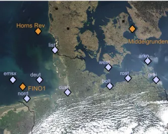
For offshore sites, the special meteorological characteristics of the marine boundary layer must be considered to predict the correct wind speed at the hub height of the wind turbines. Compared to the situation over land the situation offshore is different in three ways: the non-linear wind-wave interaction causes a variable, but low surface roughness, the large heat capacity of the water changes the spatio-temporal characteristics of thermal stratification, and internal boundary layers due to the land-sea discontinuity modify the atmospheric flow.

Figure 1 shows the positions of investigated sites in the North and Baltic Sea

Horns Rev west list arko emsx _deut cuxh nord bolt rost _grei FINO1 Middelgrunden

2. University of Oldenburg: Offshore

Forecast Accuracies and Wind Speed

Profiles

The investigations focused on the following topics: 1. Are offshore wind power forecasts going to be as accurate as the state of the art onshore?

2. Has the spatial smoothing of forecast errors the same size as onshore?

3. How can the vertical wind profile be modelled in different meteorological conditions in order to forecast the wind speed at hub height?

The following results are described in detail in [2.1], [2.2] and [2.3].

Investigated Forecasts

To estimate the future performance of wind power forecasts for offshore sites, we evaluated the accuracy of numerical wind speed forecasts with observations in the North and Baltic Sea. The numerical weather predictions (NWP) were provided by the German weather service (DWD, 7km horizontal resolution) and by the ECMWF (40km resolution). Since existing wind power production data from North Sea sites is not available for public research, we used wind speed observations from several meteorological stations at the coast line and from two lightships in the German Bight (Figure 1). All investigated periods and sites revealed similar wind conditions and similar forecast accuracies.

The measurements from the meteorological masts at Horns Rev (62m high) and FINO1 (103m) were also transformed to wind power with typical power curves of Multi-Mega-Watt-turbines. The mean wind speed at FiNO1, at 103m height is 9.8m/s in 2004, the mean producible power is 51% of the installed capacity.

Forecast Accuracy

We found that the accuracies of wind speed and wind power predictions provided by the European Centre for Medium-Range Weather Forecasts, ECMWF and the German weather service DWD for all investigated offshore sites are similar or better than for single onshore sites, considering that the mean producible power is twice as high as onshore.

Fig. 2.1: Error parameters of ECMWF forecasts

transformed to Power at FiNO1, 103m height, complete

year 2004.

Although it was found that ECMWF forecasts have a higher accuracy than DWD forecasts, a weighted combination of the two forecast sources leads to reduced errors: A combined power prediction for a single site in the North Sea with a hub height of 100m shows a relative root mean square error of 16% of the rated power for a look-ahead time of 36h. (Fig 2.2)

Forecasts of 25GW Wind Power in the North Sea

Previous investigations for onshore wind power have shown that a regional forecast has lower errors than a forecast for a single site. The relative prediction error for the aggregated power output of many wind farms in a region decreases for increasing region size as single errors are less correlated, a general effect in NWP. This reduction occurs even when the number of wind farms in the regions stays constant. How strong is the effect for offshore predictions?

To evaluate ECMWF forecasts at 22 projected sites in the German Bight (Figure 2.3), we used the regional weather analysis from DWD as a substitute for onsite observations. The spatial decay of the correlation of forecast errors has the same strength as onshore. (Fig 2.4)

Fig. 2.2: RMSE of power forecasts based on DWD, ECMWF and their combination at FiNO1, at 103m height, complete year 2004.

Fig. 2.3: Red areas mark the sites for all offshore projects in the German Bight with official applications. Source: www.bsh.de.

Fig. 2.4: Scatter dots: Correlation between the forecast errors at two out of 22 offshore sites vs. their distance in km. Lines: Binned values. Blue: forecast time 12h, Green: 36h, Pink: 48h.

Aggregated 25GW Forecasts

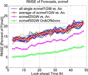
The regional forecast for a total capacity of 25GW in the German Bight shows an RMSE of 9-17%, credited to spatial smoothing effects that reduce the error by a factor of 0.73 compared to a single site. Hence, a combined regional forecast for all offshore sites would show an RMSE of 12% at 36h forecast time, i.e. an absolute RMSE of 3GW.

What is the respective spatial error smoothing for the sum of onshore and offshore wind farms in Germany? We calculated an aggregated forecast for a situation with 25GW installed offshore capacity and 25GW onshore for the year 2004. As a reference, we used the sum of the offshore wind power time series calculated from the weather analysis and the real German onshore wind power production time series from 2004 that was scaled from 17GW to 25GW. The resulting RMSE ranges from 5% to 10% (Figure 2.5), i.e. the area size of 800km leads to an error reduction factor of 0.43 for a total installed capacity of 50GW.

Fig. 2.5: RMSE of ECMWF wind power forecasts. Thin lines: all single 22 sites. Red triangles: Average of single sites. Pink stars: Aggregated 25GW offshore forecast. Green circles: Aggregated 50GW on-&offshore forecast.

Description of the vertical wind speed profiles in offshore conditions

Fig. 2.6 and 2.7 illustrate that measured wind shears and profiles deviate from those produced by weather forecast models. This effect can be detected for all different weather situations and indicates the need for a more detailed description of the marine boundary layer [2.1, 2.2].

Fig. 2.6: Mean measured and predicted wind profiles at Horns Rev; average of winter period, log. scale.

Fig. 2.7: Mean measured sea sector (190° - 250°) wind profile at FINO1 in 2004 compared to the mean output of two mesoscale models for the same wind directions: DWD-Lokalmodel and MM5-Simulation.Linear scale.

For an improved simulation of the vertical wind speed profiles, we developed a new analytic model of marine wind velocity profiles.

In our new air-sea-interaction model called ICWP (Inertially Coupled Wind Profiles, Fig. 2.8), we couple the Ekman layer profile of the atmosphere to the wave field via a Monin-Obukhov corrected logarithmic wind profile in between [2.2].

Fig. 2.8: Scheme of the vertical wind profile used in the ICWP model.

In particular, the flux of momentum through the Ekman layers of the atmosphere and the sea is described by a common wave boundary layer. The good agreement between our theoretical profiles and observations at Horns Rev and FINO1 support the basic assumption of our model that the atmospheric Ekman layer begins at 10 to 30m height above the sea surface (Fig. 2.9, 2.10). With this approach, it is possible to refine the vertical resolution of NWP profiles in a better way than with standard formulas.

Fig. 2.9: Mean measured “open sea” sector (135° - 360°) wind profile at Horns Rev compared to mean of ICWPs and average offshore WAsP profile. Period 10/2001-04/2002.

Fig. 2.10: Mean “open sea” wind profiles at FINO1 for the undisturbed sector (190° - 250°) and wind speeds greater than 4 m/s at 103m height: Obs. compared to different profile schemes. Averages of year 2004.

Acknowledgements

We like to thank DWD, ECMWF, BSH, Germanischer Lloyd, DEWI and winddata.com that kindly provided forecast and measurement data.

References

[2.1] Tambke J, Lange M, Focken U, Wolff J-O, Bye JAT. Forecasting Offshore Wind Speeds above the North Sea. Wind Energy 2005; 8: pp. 3-16.

[2.2] Tambke J, Claveri L, Bye JAT, Lange B, von Bremen L, Durante F, Wolff J-O. Offshore Meteorology for Multi-Mega-Watt Turbines. Scientific Proc. EWEC, Athens, 2006

[2.3] Tambke J, Poppinga C, von Bremen L, Claveri L, Lange M, Focken U, Bye JAT, Wolff J-O: Advanced Forecast Systems for the Grid Integration of 25GW Offshore Wind Power in Germany. Scientific Proc. EWEC, Athens, 2006

3. Overspeed GmbH: Statistical

characteristics of offshore wind speed and

prediction time series

Goals and tasks

For offshore applications, one goal is to produce forecasts for single wind farms which cover a large area. E.g. in Germany, a typical size of new offshore wind farms is 80 turbines. Obviously, some meteorological conditions differ significantly between on- and offshore. On the sea, the vicinity of the wind farm is characterized by a very uniform, almost homogeneous roughness. Because large wind farms are installed on a limited area, gradients of power output could be significantly higher than for on-shore farms.

Due to the limited possibility of measurements at off-shore wind farms, we make a detailed analysis of the statistical behavior of wind speed measurements and predictions. Complementary to the previous section, the characteristics of each single time series is in the focus, and not the analysis of the forecast error, i.e. the difference time series between measured and predicted values.

Data basis

For the analysis, we used the three time series from section 2 for the forecast range from 1h to 24h:

- measured wind speed at the German FINO1 offshore platform (cup anemometer, 103m height) (“FINO”) - predictions from the German Lokalmodell, nearest grid point, 1 hour means, grid size 7x7 km2, (“DWD”) - ECMWF predictions, nearest grid point, 3 hourly values, interpolated to 1 hour, grid size 40x40 km2 (“ECMWF”).

Average values

FiNO DWD ECMWF

Average [m/s] 9.7 9.7 9.6 Stand. Dev. STD [m/s] 4.8 4.9 4.8

Table 3.1 Overall statistical values

The global statistical values average and standard deviation STD show an astonishing good accordance. Also the correlation coefficients (gap = 0) are very high (see Reference [2.3]). Please note that there was no correction or additional detailed modeling. All values were taken directly from the prediction models.

Power Spectra

Figures 3.1 and 3.2 show the power spectral density (PSD) of all three time series, for the whole frequency range (Fig 3.1) and the high frequency part only (Fig 3.2). While FINO and DWD show a very good correlation, the ECMWF PSD has much lower values for high frequencies. Of course this is not only a “real” property of the ECMWF model, but is mainly due to the production of the time series from 3 hour sample values by interpolation. Nevertheless the “damping” seems to be a little bit stronger than it could be explained by this procedure.

Fig. 3.1 Power spectral density of all three time series.

Fig. 3.2: as 3.1, high frequencies only.

A hint is the “natural” time scale of these predictions. Depending on grid size, even the single grid point prediction values are averages over the according grid cell. Taking a grid spacing of 40 km and assuming a mean wind speed of 10 m/s, this would lead to a typical minimum time scale of 67 minutes. Taking into account that the underlying Navier-Stokes equation is of second order, the natural grid time scale is two to three times this value (depending on the numerical algorithm), i.e. 2 to 3 hours.

Gradients

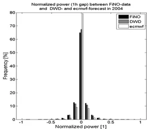
The statistical properties of time series directly reflect in the temporal (and spatial) gradients which could occur. Figure 3.3 shows the comparison of normalized gradients (differences) from hour to hour for the measured and the two predicted time series in 10 % steps. It can be clearly seen that the ECMWF forecast underestimates the larger deviations (and thus has big values for the central +/- 5% bin). Figure 3.4 shows the same presentation for power output. For this estimation, simply a theoretical power curve was applied to the wind speed values (no farm effects, no additional smoothing).

Fig. 3.3 Distribution of temporal differences of wind speed (time gap: 1 hour), norm. to mean wind speed

Fig. 3.4: Distribution of differences of power output (time gap: 1 hour), normalized to rated power.

Because the power curve is non-linear, basically higher gradients would be expected. In fact, the relative gradients are smaller. This effect is due to the fact that the mean wind off-shore is very high compared to usual land wind farm sites (here: approx. 10m/s). This leads to the fact that the turbines are operating near their rated wind speed (here: 14m/s). So fluctuations to higher wind speeds are damped, not amplified. On the other hand side, if the wind speed is above rated, a negative fluctuation produces no or small gradients.

Conclusion

Even from this basic investigation it can be seen that: • the time domain behavior must be analysed

properly to evaluate how a predicted time series shows critical behavior like maximum gradients

• the influence of the specific power curve is very high because off-shore turbines are working close to their rated wind speed quite frequently.

For predicting whole wind farms covering areas of several hundred square kilometers, it is important to analyse the spatial behavior of the predictions accordingly.

4. RISOE: Comparison of different offshore

effects on wind power forecasts

As large offshore wind farms in the hundred’s of megawatt class are developed, a number of special issues arise in terms of forecasting power output. As part of Anemos wind farm and boundary-layer models were reviewed which could be utilised to predict power output from turbines within and downwind of large offshore wind farms [4.1]. A new model was developed which models wakes within wind farms by conserving momentum deficit [4.2]. The remainder of the work focused on quantifying the impact of corrections to short-term forecasts of power output from large offshore wind farms. The effects considered are: wind speed gradients in the coastal zone, vertical wind speed profile extrapolation to hub-height and wake effects. On the positive side wind speeds offshore in the power producing classes appear to be more persistent, with lower probability and persistence of calms [4.3]. On the other hand, the development of wind farms in coastal areas (<50 km to the coast) where wind speed gradients and profiles are still developing may mean that additional corrections are needed to ‘traditional’ approaches to short-term forecasting.

Horizontal wind speed gradients

These gradients were examined using mesoscale models, satellite observations and linearized models [4.4]. At distances of more than about 20 km from the coast wind speed gradients are unlikely to be important except possibly in very stable conditions. Closer to the coast gradients were shown to be strongly related to the temperature difference between land and sea and to be significant even over the area of a 100+ turbine wind farm implying that using one central grid point will lead to errors in the forecast wind and therefore in power output.

Horizontal and vertical temperature gradients

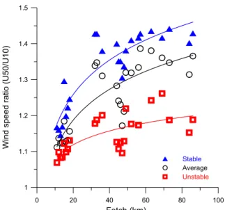
Both gradients influence the wind resource more strongly offshore because ambient turbulence is lower than it is over most land surfaces [4.5]. The stability climate at a particular site seems to be strongly synoptic with a smaller influence of the fetch (defined here as the distance to the coastline) assuming the wind farm is placed beyond 10 km from the nearest coast [4.6]. As shown in Figure 4.1 (based on data from Nysted) the wind speed profile takes much longer time/distance to reach equilibrium in stable than near-neutral or unstable cases. A new method of calculating stability using the wind shear instead of using heat flux or accurately measured temperature gradients was developed and shown to be adequate, unless there are strong horizontal wind speed gradients (usually in short distances to land where conditions are not at equilibrium) [4.4]. In this case the method fails because the large wind shear implies stable conditions. At Horns Rev (Figure 4.2), the measured wind speed profile implies wind speed profiles become linear above heights of about 50 m which might suggest that the constant flux layer theory is inadequate [4.7]. 0 20 40 60 80 100 Fetch (km) 1 1.1 1.2 1.3 1.4 1.5 W in d speed ratio (U50 /U1 0 ) Stable Average Unstable

Figure 4.1. Ratio of wind speeds at 50 m to those at 10 m height for different fetches and stability conditions.

1 1.04 1.08 1.12 1.16 1.2

Normalised wind speed 10 100 20 30 40 50 60 70 80 90 He ig h t ( m ) Observed Stability corrected Logarithmic

Figure 4.2. Comparison of normalised wind speed profiles at Horns Rev.

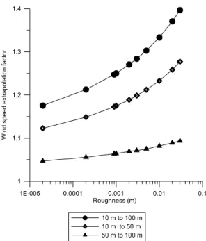
Sea surface roughness

The role of changing roughness offshore is thought to be minor. Even quite large changes in a low roughness make a very small difference to the extrapolation of wind speeds from 10 m to turbine hub-heights as shown in Figure 4.3. Clearly using data from the measured or modelled height closest to hub-height is preferable and will result in the lowest errors. Wind speeds may also be extrapolated from a model layer e.g. at 100 m down to turbine hub-heights. In some circumstances (e.g. using buoy data from 2m height) the choice of roughness length will have a profound impact on the predicted wind speed.

1E-005 0.0001 0.001 0.01 0.1 Roughness (m) 1 1.1 1.2 1.3 1.4 W ind s pee d e xt rap ol at io n f a ct o r 10 m to 100 m 10 m to 50 m 50 m to 100 m .

Figure 4.3. Wind speed extrapolation factor based on a logarithmic profile for different heights and roughnesses.

Stability correction at Middelgrunden

Use of the prediction with the stability correction at Middelgrunden gives slightly higher power output than the use of the logarithmic prediction (Figure 4.4). In order to evaluate the short-term forecasts over 48 hours, the power output is calculated using the 10m forecast wind speed and either the log. profile or the stability corrected profile where the stability correction is calculated for hour zero and then applied to the subsequent 48 hours. A bias of 0.5 m/s was added to the HIRLAM 10 wind speed from which both were calculated. As shown use of the stability correction gives only a minor improvement.

0 10 20 30 40 50 Time (hour) 360 400 440 480 520 Po w er o ut put ( kW) -40 0 40 80 120 m ean e rr o r ( kW) Observed 70 m log 70 m stability mean error log mean error stability

Figure 4.4. 48 hour observed and predicted power output for a turbine at Middelgrunden (average of 351 test runs).

Wakes

Wakes within a large offshore wind farm are predicted to cause power losses of the order 10% [4.8]. This depends on many factors such as the turbine orientation and spacing, wind climate and turbine type. However, most wake models were developed for single wakes and there are substantial differences between the wake losses predicted for single wakes [4.9], [4.10] although the best results in terms of model agreement and model agreement with limited data sets is at moderate turbulence and moderate wind speeds. Prediction of multiple wakes likely requires feedback between wake and boundary-layer development [4.11]. However, what remains to be done here is to assess whether a look-up table of wake losses by wind speed/direction is as accurate as use of a simple wake model in a short-term forecasting context.

References

[4.1] Barthelmie, R.J., et al. Analytical and empirical modelling of flow downwind of large wind farm clusters. in The science of making torque from wind. 2004. Delft. [4.2] Frandsen, S., et al., Analytical modelling of wind speed deficit in large offshore wind farms. Wind Energy 2006. 9(1-2): p. 39-53.

[4.3] Pryor, S.C. and R.J. Barthelmie, Comparison of potential power production at on- and off-shore sites. Wind Energy, 2001. 4: p. 173-181.

[4.4] Barthelmie, R.J., G. Giebel, and J. Badger. Short-term forecasting of wind speeds in the offshore environment. in ‘Copenhagen Offshore Wind 2005’, Copenhagen, October 2005. 2005.

[4.5] Motta, M., R.J. Barthelmie, and P. Vølund, The influence of non-logarithmic wind speed profiles on potential power output at Danish offshore sites. Wind Energy, 2005. 8: p. 219-236.

[4.6] Motta, M., R.J. Barthelmie, and P. Vølund, Stability effects on predicted wind speed profiles and power output at the Vindeby offshore wind farm. Wind Eng Journal, 2003.

[4.7] Tambke, J., et al., Forecasting offshore wind speeds above the North Sea. Wind Energy, 2005. 8: p. 3-16.

[4.8] Barthelmie, R., et al., ENDOW: Efficient Development of Offshore Windfarms: modelling wake and boundary-layer interactions. Wind Energy, 2004. 7: p. 225-245.

[4.9] Rados, K., et al., Comparison of wake models with data for offshore windfarms. Wind Engineering, 2002. 25: p. 271-280.

[4.10] Schlez, W., et al., ENDOW: Improvement of wake models within offshore windfarms. Wind Engineering, 2002. 25: p. 281-287.

[4.11] Frandsen, S., et al. Analytical modelling of wind speed deficit in large offshore wind farms. in European Wind Energy Conference and Exhibition. 2004. London.

5. Ecole des Mines: Contribution of

satellite-radar information for offshore forecasts

The most interesting satellite data for this objective of the ANEMOS project are coming from radar sensors. These sensors are active sensors, carrying their own power source. This allows them to acquire data at any time of the day, with any kind of weather. The sensors of interest in the framework of the project are the scatterometers and the synthetic aperture radars (SAR). The benefits of these sensors for wind prediction were analysed during the project.

From empirical models, the CMODs, it is possible to obtain spatially distributed wind speeds and directions from these sensors. The quality of the data was evaluated and uncertainties computed for the creation of wind parameter maps based on this data set (Ben Ticha and Ranchin, 2006).

These wind data extracted from the satellites are the basis of the proposed methodology for use of satellite data in wind predictions.

Methodology

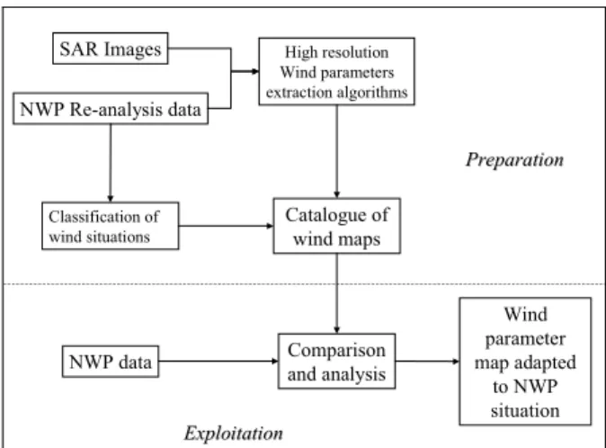
We try to take advantage of all the available data in order to construct a distribution map of wind patterns according to the wind prediction provided by the Numerical Weather Prediction (NWP). In other words, we try to construct a catalogue of wind field distribution, which can be used to propose a map according to the wind prediction provided by the meteorological models. Figure 5.1 proposes such an example. In order to propose a spatial distribution of the wind patterns according to the NWP, it is necessary to construct a catalogue of these patterns in the area of interest. This is done by processing the available archive of SAR images in the area of the offshore case study. The NCEP/NCAR reanalysis data1 _is

used for construction of the catalogue of typical wind situations. The SAR images are first processed in order to deliver the wind patterns. Considering the meteorological situation at the acquisition time (coming from the NCEP/NCAR data) of the SAR images, the wind patterns are classified. The classification allows linking a specific NWP to a specific wind pattern distribution coming from SAR. The construction of the catalogue of the wind patterns will allow the computation of quality parameters based on the probability distribution function (pdf) of the NWP case. Figure 5.2 presents the flowchart for the preparation and exploitation of the SAR information for prediction. Figure 5.3 proposes an example of the different wind situations encounters in the area of interest. For each typical wind situations, a wind pattern is associated and a wind pattern distribution proposed for the area of interest.

Reference

Ben Ticha M.B., Ranchin T., 2006. Offshore wind resource assessment using satellite data: uncertainties estimation. Proceedings of the European Wind Energy Conference EWEC, Athens, 2006.

1

_{NCEP/NCAR Global Reanalysis Products:}

http://dss.ucar.edu/datasets/ds090.0/

Figure 5.1. Example of a specific wind pattern derived from satellite data at Arklow Bank, Irish Sea, 19th _April

2003. SAR Images NWP Re-analysis data High resolution Wind parameters extraction algorithms Classification of wind situations Catalogue of wind maps

NWP data Comparison _{and analysis}

Wind parameter map adapted to NWP situation Preparation Preparation Exploitation Exploitation

Figure 5.2 Flowchart of preparation and exploitation of SAR images in offshore prediction.

Figure 5.3 Typical wind situations derived from the NCEP/NCAR data set

0 2 4 6 8 10 12 14 16 W ind speed (m/s)

6. CIEMAT: The Tarifa model for the Strait

of Gibraltar

CIEMAT has developed a semi-empirical model that is valid for the Strait of Gibraltar, although the method can be applied to any other place.

The Strait of Gibraltar is a very important place regarding wind energy, because of its great potential and installed power (onshore by now), but it is also the place where the highest errors in wind prediction take place. Thus, the importance of finding a model that improves the current predictions (i.e. Hirlam or ECMWF) is evident.

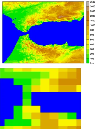
Fig. 6.1. Comparison of 2x2 km (top) and 50x50 km (bottom) resolution topographies of the Strait of Gibraltar

One of the reasons because the ECMWF global model does not give good enough wind predictions at the Strait is the model resolution. In Figure 6.1 the quasi-real topography of the Strait (2x2 km) is compared with the

topography used by the ECMWF model (approximately 50x50 km). It is easy to understand the impossibility of reproducing the flow across the Strait (there is not even a channel!). In fact this global model sometimes predicts strong meridian component winds that actually are not observed at the Strait.

After having analysed very carefully the wind regime at the Strait [6.1, 6.2], it has been concluded that there is a direct relation between the low-level meteorological patterns (represented by significant atmospheric variable fields) and the surface wind across the Strait, and this relation is not always the usual one. For instance, there are times when the wind is isobaric and other times when it is transisobaric. This fact suggested using a tool that could take into account this relation. Therefore the Perfect Prognosis (P.P.) technique has been chosen. This method uses multivariate regression analysis in order to get an equation that show this relation between the surface wind speed (dependent variable) and other atmospheric independent variables Vi (predictors) derived

from the operational ECMWF model analysis: WIND SPEED= C0 + C1V1 + C2V2 + C3V3 + ... CnVn

Thus, the objective is finding the best predictors Vi

(explaining most of the observed variance) and the corresponding coefficients Ci of the multiple regression

equation. In this case, a backward stepwise method has been chosen. The empirical wind speed data used in this work have been collected from the meteorological station in Tarifa (Spain), just near the coast (Fig 6.2) during the 1995-97 years. The independent variables used come from the ECMWF reanalysis (ERA data) for the same period.

They can be individual atmospheric variables at diverse p-levels or appropriate combinations of them, taking into account previous knowledge about the qualitative relation between these variables and the resultant local-scale wind. The ERA data used correspond to different nodes of a 0.5°x 0.5° lat-lon grid mesh in the vicinity of Tarifa station, as Figure 6.2 shows.

Taking into account the previous knowledge of the wind regime at the Strait, 10 sub-groups or cases were considered: four corresponding to the easterly winds for the 4 seasons, four to the westerly winds for the 4 seasons and two for the easterly and westerly “calms” (v< 1 m/s). Fig. 6.2. Map of the Strait of Gibraltar with the nodes of the ECMWF model grid mesh. The location of the Tarifa meteorological station corresponds to the 642 node.

EASTERLIES WESTERLIES Calms Spring Summer Autumn Winter Spring Summer Autumn Winter Easterlies Westerlies

N. of samples 518 434 465 278 411 454 442 565 173 214 Adjusted R2 _{.72 .74 .72 .79 .62 .54 .54 .67 .50 .35}

Standard error of

estimates 2.41 2.17 2.04 2.21 2.26 2.40 2.38 2.43 2.40 2.18 Table 6.1: Statistical regression results, including the

number of samples, the adjusted R2 _{and the standard}

error of estimates values for each one of the ten considered cases.

Table 6.1 shows the number of samples, the multiple determination coefficient corrected by freedom degrees (R2_{) and the standard error of estimates for each one of}

the 10 considered cases.

In order to validate the Tarifa model, the ECMWF model forecasting daily data at 24h, 36h and 48h horizons for the whole 1997 year were considered. The regression equations obtained from the P.P. technique were applied

to forecasts, and wind estimations were compared to observed values at the Tarifa station.

Table 6.3 shows the mean square errors of wind predictions from the ECMWF model before and after the Tarifa model was applied. These have been calculated for different wind speed intervals and for the three horizon predictions (24h, 36h and 48h). The number of data corresponding to each case is also included. It can be seen that the ECMWF model wind speed prediction errors are much higher than the Tarifa model ones. It can be concluded that the Tarifa model is an adequate downscaling technique which greatly reduces the errors in wind forecasting at the Strait of Gibraltar.

Horizon SPEED INTERVALS 1-5 m/s /U1000/>1 5-10 m/s 10-15 m/s > 15 m/s TOTAL CALMS /U1000/<1 Mean square error (m/s) 1.99 3.00 2.79 3.28 2.94 4.25 24h Number of samples 20 136 103 55 314 40 Mean square error (m/s) 2.32 3.44 3.27 4.14 3.25 3.66 36h Number of samples 60 114 89 50 313 40 Mean square error (m/s) 2.55 3.20 3.99 3.47 3.39 3.50 48h Number of samples 19 141 97 56 313 39 Horizon SPEED

INTERVALS /U1000/>1 1-5 m/s 5-10 m/s 10-15 m/s > 15 m/s TOTAL /U1000/<1 CALMS Mean square error (m/s) 7.07 8.36 7.16 -- 7.53 4.77 24h Number of samples 200 101 13 0 314 40 Mean square error (m/s) 5.73 8.34 6.54 -- 6.51 2.97 36h Number of samples 223 81 9 0 313 40 Mean square error (m/s) 6.65 8.18 7.14 -- 7.19 5.14 48h Number of samples 205 100 8 0 313 39

Table 6.3: Number of samples and mean square errors corresponding to different speed intervals and

forecasting horizons for the statistical regression model (up) and the ECMWF model (down) during the 1997 year.

References

[6.1] Palomares A. M., Study of wind conditions and mesoscale turbulence in Tarifa (Spain).Proc. E.C. Wind Energy Conference .Madrid, Spain 1990.

[6.2] Palomares A.M., Analysis of the meteorological synoptic situations that affect the Strait of Gibraltar and their influence on the surface wind. Spanish Ocean. Inst Bull.15 (1-4) Spain 1999: 81-90.

7. Ecole des Mines:

Test Case Middelgrunden, Denmark

In this section the case study of the Middelgrunden offshore wind farm in Denmark is presented. The wind farm, which was built in 2000, is situated a few kilometres away from Copenhagen. It contains 20 Bonus wind turbines rating 2 MW each.

The available data are measurements of the average hourly power production of the wind farm as well as of the wind turbines. To overcome the difficulty of different commissioning dates of the wind turbines, the total production if scaled to the final total capacity according to the number of commissioned wind turbines.

Hirlam Numerical Weather Predictions (NWPs) from the Danish Meteorological Institute are used. They are composed of the following data: 10m wind speed, wind direction and air density. The NWPs are delivered twice a day with a 3 hours resolution and cover a period of 48 hours. For sake of compatibility with the power measurements, the NWP data have been interpolated for obtaining a hourly resolution.

The period of the study ranges from the 9th _{of February}

2001 to the 15th _{of October 2002.}

7.1 Advanced Statistical Modelling Using Artificial Intelligence Based Methods

For this study the AWPPS (ARMINES Wind Power Prediction System) model was used. The core of this model consists of a fuzzy neural network (NN). The F-NN is generic and can be trained on appropriate input depending on the final use of the model. Regarding measurements, only the scaled total production was used as input.

In the F-NN model, Gaussian fuzzy sets Ai are defined

over the explanatory variables (x1 , …, xn). Fuzzy rules are

derived linking the input fuzzy sets to the prediction output. These fuzzy rules may have the form :

IF x1 is A1 and … and … xn is An THEN yi=f(x1 , …, xn)

Each rule provides an estimation of the prediction output y according to its local “perception” yi of the situation.

The resulting forecasts are derived from these estimations. The advantage of this model compared to conventional neural networks is that it permits to model the process of interest locally. Local modelling is desired if one is forecasting non-stationary processes such as wind generation. Special attention is made to develop robust algorithms for estimating the models' parameters.

7.2 Results

The available data have been separated to a learning, validation and testing set. The learning set, used for the model's parameters estimation, covers a period of about 5.5 months (up to the 25th _{of July). The parameters}

estimation was done using appropriate learning rules that minimize error while at the same time maximize entropy. The validation set covered a period of 3 months (up to the 26th _{of October). It was used to take automatically}

decisions on the structure of the model using the cross-validation method generalized upon the whole prediction horizon. Finally, the remaining data of 12 months have been used for the final evaluation of the model. The results on the testing set are presented below.

In order to obtain results which are comparable with the ones delivered by physical prediction models, the evaluation was based on the 00h and the 12h runs of the model. The predictions used correspond to the reception of the NWPs.

For validating the results obtained, the persistence model has been used as a benchmark.

0 5 10 15 20 25 30 35 40 0 3 6 9 12 15 18 21 24 27 30 33 36 39 Look-ahead time (h) N M AE ( % of nom inal po w e

r) Persistence (Middelgrunden)_{Advanced model (Middelgrunden)}

Advanced model (Tuno Knob)

Figure 7.1: Normalized Mean Absolute Error (NMAE)

Figure 7.1 compares the performance of the advanced model to that of Persistence on the testing set using the Normalised Mean Absolute Error (NMAE). Normalization is made on the basis of the nominal capacity of the wind farm. The advanced model outperforms Persistence for all horizons. The upward trend of the prediction errors grows slowly. The normalized error only increments by 3.2% between horizons 6 and 36. The results are comparable to the ones obtained from the offshore Tunø Knob wind farm considered in [7.1] for the benchmarking of 8 advanced physical and statistical models, regarding the fact that the mean produced power at Tunø Knob is higher.

Normalised RMSE 0 5 10 15 20 25 30 35 40 1 3 5 7 9 11 13 15 17 19 21 23 25 27 29 31 33 35 37 Look-ahead Time (h) Pe rc e n ta g e of Nom ina l Powe r Persistence F-NN

Figure 7.2: Normalized Root Mean Square Error NRMSE at Middelgrunden

7.3 Conclusion

The F-NN model of the AWPPS prediction module shows an improvement over persistence from the first time step. Moreover, the normalized error grows slowly with the horizon. The model performed well whatever horizon is considered. The mean power production per horizon was found very close to the reference power and the power cycle. The F-NN model, being generic, permits to test alternative configurations that include the horizon as an input variable in order to better catch the wind power

diurnal cycle. Another possibility is to consider a different model for each horizon (or ensembles of horizons).

The artificial intelligence approach considered here is judged as adequate for modelling large size offshore wind farms. In the future, in very large wind farms of several tens or hundreds of MW, the challenge will be to capture in an adequate way spatio-temporal behaviour. As a perspective, and as a function of available data, one could consider appropriate model set-ups for large wind farms such as clustering-based approaches. Then, the objective would be to predict the production of a group of wind turbines forming a cluster. A specific model could be tuned for each cluster as shown in the following Figure 7.3.

Figure 7.3: Possible model configuration for very large

offshore wind farms.

References

[7.1] Kariniotakis, G., I. Marti, et al, "What Performance Can Be Expected by Short-term Wind Power Prediction Models Depending on Site

Characteristics?", In: CD-Rom Proceedings, European Wind Energy Conference EWEC 2004, London, UK, 22-25 Nov. 2004.

[7.2] Pinson, P., Kariniotakis, G., Ranchin T., Mayer, D., "Short-term Wind Power Prediction for Offshore Wind Farms - Evaluation of Fuzzy-Neural Network Based Models", CD-Rom Proceedings of the Global WindPower 2004 Conference, Chicago, USA, 28-31 March, 2004.

[7.3] Kariniotakis, G., Pinson, P., Giebel, G., Bartelmie, R., The state of the art in Short-term Prediction of wind Power - From an offshore Perspective, In: CD-Rom Proceedings, Symposium ADEME, IFREMER, "Renewable energies at sea", Brest, France, October 20-21, 2004.

8. RAL: Application of RAL forecasting

model to the Middelgrunden offshore wind

farm

8.1 Introduction

RAL have developed a wind power forecasting model which uses information both from on-line measurements of wind farm output power and from numerical weather prediction models. The model can be clased as an initial-(value)-boundary-value model as it uses both ’internal’ and ’external’ variables. The structure of the IBV model is briefly outlined in Section 8.2 and the performance of the model when applied to the Middelgrunden offshore wind farm is presented in Section 8.3.

8.2 The Initial-Boundary-Value model

Model structure

In the IBV model, the measured sequence of data

(

t

k

)

y

+

is represented in terms of the of the observed historical sequence of data,

y

( )

t

-

n

, and the history of external forces acting,

x

_j

(

t

+

k

-

m

)

, in terms of constant coefficient auto-regressive mapping parameters,

g

_n,k , the response function to external excitations,

k m, j,

h

, and a stochastic variable

r

(

t

+

k

)

with

( ) ( )

t

k

r

t

k

g

y

( )

t

-

n

+

h

x

(

t

k

-

m

)

y

J _{j,m,k j} 1 j M 0 = m k n, N 1 n

∑

∑

∑

+

+

+

=

+

= =

The optimum values for

g

_n,k and

h

_j,m,k are estimated by taking moments <y(t)zi(t-k)>, where z and k

represent generically the range of external variables and delays in the model, and solving the resulting matrix equation for

g

_n,k and

h

_j,m,k by linear least-squares regression.

In the present case, the variable y represents the measured wind power output and the variables xj functions of

external variables such as forecast wind speed, forecast wind direction and time of day. Wind power forecasts y(t+k) are generated from the measured data y(t) and the forecast variables xj using the coefficients

g

_n,k and

k m, j,

h

for each separate forecast horizon k.

Two different models were applied to the Middelgrunden case. In both models, only the most recent power measurement y(t) was used, corresponding to an AR(1) model. The forecast wind speed was included as a cubic, representing an empirical approximation to the wind farm power curve :

∑

=

=

3 0 n n n 3

(v)

a

v

P

In the second model additional terms in the forecast wind direction Θ and time of day τ were included as second-order harmonic series:

)

n

sin(

s

)

n

cos(

c

)

(

H

2 _n 1 n n 2

θ

=

∑

θ

+

θ

=

and similarly for

H

₂

(

τ

)

.

The two IBV models applied to the training data set for Middelgrunden (16/10/2001 00:00 - 15/10/2001 23:00) were :

• AR(1) + P3(v)

• AR(1) + P3(v) + H2(Θ) + H2(t)

Forecasts were updated with each new SCADA value, at 1-hour resolution. The NWP forecast from the Danish Meteorological Service HIRLAM model for 10 m was used, interpolated from a 3-hour resolution to 1 hour. The length L (days) of the out-of-sample data series over which the moments <y(t)zi(t-k)> are taken was set to 50

days.

8.3 Results

The results for the AR(1) + P3(v) + H2(Θ) + H2(t) model

are shown in Fig. 8.1. The performance of the ‘naïve’ or ‘persistence’ predictor (which predicts y(t+k) = y(t)for all k) is shown for comparison.

The performance of the AR(1) + P3(v) + H2(Θ) + H2(t) is

compared to that of the simpler AR(1) + P3(v) in Fig. 8.2.

The figure shows the correlation coefficient r2 between forecast and observed wind power, as a function of

horizon, over the evaluation period. The inclusion of forecast wind direction and time-of-day as predictors gives only a small improvement in model performance, consistent with the expectation that an offshore site is unlikely to be subject to large local diurnal or topographical effects. Middelgrunden 0,00 0,05 0,10 0,15 0,20 0,25 0,30 0,35 0,40 0 6 12 18 24 30 36 Horizon / hours No rm al is e d RM S E Persistence IBV model

Figure 8.1 : RMS errors for the IBV and persistence models for Middelgrunden. The RMS errors have been normalised to the wind farm installed capacity of 40 MW.

0,4 0,5 0,6 0,7 0,8 0,9 1 0 6 12 18 24 30 36 Horizon / hours Cor re la tion c o e ffi ci ent · AR(1) + P3(v) · AR(1) + P3(v) + H2(Θ) + H2(t)

Figure 8.2 : Correlation coefficients for the AR(1) + P3(v) and AR(1) + P3(v) + H2(Θ) + H2(t) models applied to