Bagging Stochastic Watershed on Natural Color Image Segmentation

HAL Id: hal-01104256

https://hal.archives-ouvertes.fr/hal-01104256

Submitted on 18 Mar 2015

HAL is a multi-disciplinary open access

archive for the deposit and dissemination of

sci-entific research documents, whether they are

pub-lished or not. The documents may come from

teaching and research institutions in France or

abroad, or from public or private research centers.

L’archive ouverte pluridisciplinaire HAL, est

destinée au dépôt et à la diffusion de documents

scientifiques de niveau recherche, publiés ou non,

émanant des établissements d’enseignement et de

recherche français ou étrangers, des laboratoires

publics ou privés.

Segmentation

Gianni Franchi, Jesus Angulo

To cite this version:

Gianni Franchi, Jesus Angulo. Bagging Stochastic Watershed on Natural Color Image Segmentation.

International Symposium on Mathematical Morphology and Its Applications to Signal and Image

Processing, 2015, Reykjavik, Iceland. pp.422-433, �10.1007/978-3-319-18720-4_36�. �hal-01104256�

on Natural Color Image Segmentation

Gianni Franchi and Jes´us Angulo

MINES ParisTech, PSL-Research University, CMM-Centre de Morphologie Math´ematique; France

gianni.franchi@mines-paristech.fr,jesus.angulo@mines-paristech.fr

Abstract. The stochastic watershed is a probabilistic segmentation ap-proach which estimates the probability density of contours of the image from a given gradient. In complex images, the stochastic watershed can enhance insignificant contours. To partially address this drawback, we introduce here a fully unsupervised multi-scale approach including bag-ging. Re-sampling and bagging is a classical stochastic approach to im-prove the estimation. We have assessed the performance, and compared to other version of stochastic watershed, using the Berkeley segmentation database.

Keywords: unsupervised image segmentation ; stochastic watershed; Berkeley segmentation database

1

Introduction

The goal of image segmentation is to find a simplified representation such that each pixel of the image belongs to a connected class, thus a partition of the image into disjoint classes is obtained. One can also talk of region detection. We would like to emphasize from the beginning the difference between this type of technique and edge detection. Indeed the contours obtained by edge detection are often disconnected and may not necessarily correspond to closed areas.

In this paper, we introduce a new variant of the stochastic watershed [2] to detect regions and also to calculate the probability of contours of the edges of a given image. Inspired by the milestone segmentation paradigm of Arbelaez et al._{[4] and in order to improve the results, we will combine some of their tools,} like the probability boundary gradient or the spectral probability gradient, with the morphological segmentation obtained by the stochastic watershed. The work that we present can be applied to both gray-scale and color images. Our main assumption here is that the approach should be fully unsupervised. In order to quantitatively evaluate the performance of our contributions, we have used the benchmark available in the Berkeley Segmentation Database (BSD) [11].

Besides the classical contour detection techniques, such as the Sobel filter, the Canny edge detector or the use of a morphological gradient, based exclu-sively on local information, an innovative and powerful solution is the globalized probability of boundary detector (gPb) [4]. In this case, global information is

added to the local one thanks to a multi-scale filter and also by means of a no-tion of texture gradient. However, supervised learning has been used to optimize gPb which could limit its interest for other type of images than the natural color images. We note also that in [4] the gPb can be the input for a ultrametric con-tour map computation, which leads to a hierarchical representation of the image into closed regions. This approach is somehow equivalent to the use of watershed transform on a gradient since a hierarchy of segmentation is obtained [13, 14].

The interest of the stochastic watershed is to be able to estimate the proba-bility density of contours of the image from a given gradient [2, 14, 15]. However, in complex images as the ones of the BSD, the stochastic watershed enhances insignificant contours. Dealing with this problem has been the object of recent work, see [5] or [9]. We propose here a multi-scale solution including bagging. The interest of a pyramidal representation is widely considered in image pro-cessing, including for instance state-of-the-art techniques such as convolutional networks [8]. Re-sampling and bagging [7] is a classical stochastic approach to improve the estimation.

2

Background

2.1 Basics on watershed transform for image segmentation

Mathematical morphology operators are non-linear transforms based on the spa-tial structure of the image that need a complete lattice structure, i.e. an order-ing relation between the different values of the image. This is the case of ero-sion/dilation, opening/closing, etc. but also for the watershed transform (WT) [6, 12, 16, 13], which is a a well known segmentation technique. Consider that we are working in a gray scale image, and that all image values are partially or-dered, so it is possible to represent the image as a topographic relief. WT starts by flooding from the local minima until each catchment basin is totally flooded. At this point, a natural barrier between two catchment basins is detected, this ridge represents the contour between two regions. To segment an image, the WT is often applied to the gradient of the image, since the barrier between regions will correspond to local maxima of the gradient. Hence, in watershed segmentation the choice of the gradient is of great importance: it should represent significant edges of the image, and minimizes the presence of secondary edges. In the case of a color image, there are many alternatives to define the topographic relief function (i.e., the gradient) used for the WT.

Our practical motivation involves to identify a relevant gradient that maxi-mizes the F-measure on the Berkeley database, being also compatible with wa-tershed transforms (involving mainly local information). Hence, we have tested different gradients on the BSD, in particular some morphological color gradients [1], as well as the probability boundary and the globally probability boundary [4]. Following our different tests, we favor the probability boundary gradient, because it produces excellent results, being also unsupervised.

2.2 Probability boundary gradient (Pb)

Let us recall how the Pb gradient is computed [4]. First, the color image, which can be seen as a third order tensor, is converted in a fourth order tensor, where the first three channels correspond to the CIE Lab color space, and a fourth channel based on texture information is added. Then, on each of the first three channels, an oriented gradient of histogram G(x, θ) is calculated. To calculate the oriented gradient at angle θ for each pixel x of the image, a circular disk is centred at this pixel and split by a diameter at angle θ, see Fig. 1. The his-tograms of each half-disk are computed, and their difference according to the χ2 distance represents the magnitude of the gradient at θ. In the case of the texture channel, first, a texton is assigned to each pixel, which is a 17 dimensional vector containing texture descriptor information. The set of vectors in then clustered using K-means, the result is a gray-scale image of integer value in [1, K]. Second, an oriented gradient of histogram is computed from this image. The four ori-ented gradients are linearly combined, i.e., P b(x, θ) = 1

4 P4

iGi(x, θ), with i the number of channels, where Gi(x, θ) measures the oriented gradient in position x of channel i. Finally, the Pb gradient at x is obtained as the maximum for all orientations: P b(x) = maxθ{P b(x, θ)}.

In [4], it was also considered the so-called globalized probability of boundary (gPb), which consists in computing the Pb at different scales, then added to-gether, and finally, an enhancement by combining this gradient with the so-called spectral gradient.

Fig. 1.Computing oriented gradient of histograms for a given orientation. Figure bor-rowed from [4].

2.3 From marked watershed to stochastic watershed using graph model

Stochastic watershed (SW) was pioneered as a MonteCarlo approach based on simulations [2]. This is also the paradigm used for computing the examples given in this paper. However, in order to describe the SW, we follow the formulation introduced in [14], which considers a graph image representation of the WT and

leads to an explicit computation of the probabilities. A similar paradigm has been also used in [10] for efficient implementations.

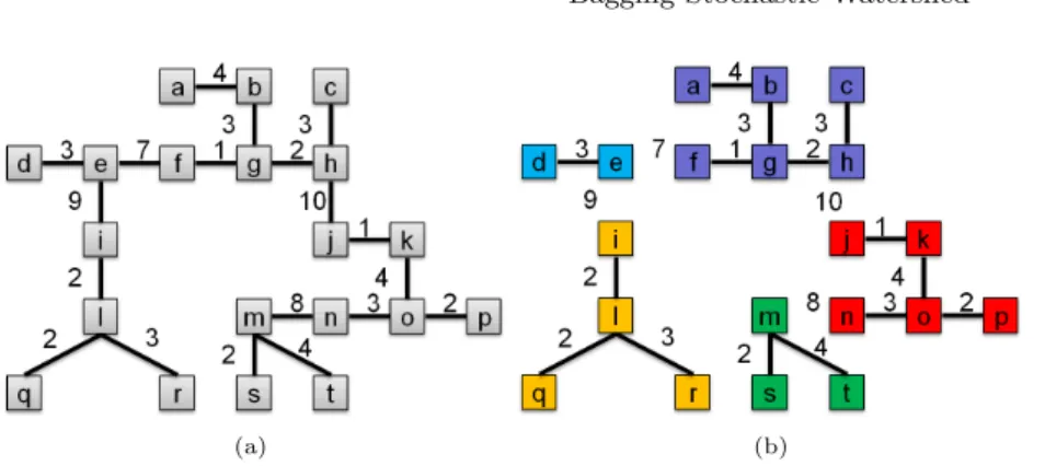
First let us consider the partitions formed by the catchment basins resulting from the WT. It is possible to work with the graph resulting from this segmenta-tion called the Region Adjacency Graph (RAG) where each node is a catchment basin of the image, and where edges are weighted by a dissimilarity between regions. In particular, the weight of the edge between two nodes is the minimum level of water λ needed so that the two catchment basins are fused. Another way to see it is to say that the weight between two nodes is the lowest pass point on the gradient image between adjacent regions. Let us now explain how to compute a marked watershed from this graph [12, 13]. First, thanks to some prior knowledge, markers are selected and play the role of sources from which the topographic surface will be flooded. Their flow is such that they create lakes. Another important point is that these markers represent the only local minimum of the gradient. Then on this new image we proceed at a WT. As previously, a region is associated to each local minimum. Another view of this problem is the RAG point of view. First, the Minimum Spanning Tree (MST) of the RAG is calculated, then between any two nodes, there exists a unique path on the MST and the weight of the largest edge along this path is equal to the flooding ultra-metric distance between these nodes. For example, if one puts three markers on the RAG then, to have the final partition, we just have to cut the two highest edges of the MST. This operation will produce a forest where each subtree spans a region of the domain. We can easily see that if one uses n > 1 markers, we would cut n − 1 edges in order to produce n trees. However markers must be chosen accurately, since the final partition depend on it. Since one may not have a priori information about the marker positions, the rationale behind the SW is to use randomly placed markers on the MST of the RAG. By using random markers, it is possible to build a density function of the contours. Let us consider an example of image with 20 catchment basins whose MST is represented in Fig 2(a). Then if one wants to calculate the probability of the boundary between the catchment basins corresponding to the nodes e and f , we will write this probability P(e, f ). One has first to cut all the edges above the value of the edge e − f , so that we get a Minimum Spanning Forest represented on Fig 2(b). Then let us consider the tree containing node e and the one containing node f that are respectively represented in purple and blue on Fig 2(b), and denoted by Te and Tf respectively. The edge e − f is cut if and only if during the process where the markers are placed randomly, there is at least one marker on Teand at least one marker on Tf.

Let us consider the node f , and let us write P(f ) the probability that one marker is placed on f such that P

ν∈VP(ν) = 1 where V is the set of all the nodes of the image, and ν is a node. Then the probability that one marker is placed on a tree T is:

P(T ) = P([ ν∈T

ν) =X ν∈T

(a) (b)

Fig. 2.(a) the Minimum Spanning Tree of on image, (b) the Minimum Spanning Forest of the same image.

One can express P(e, f ) as the probability that there is at least one marker out of N markers on Teand one on Tf, but one can also reformulate it by taking the opposite event. Then we have P(e, f ) is equal to the opposite that there is no markers on Te or on Tf. The probability that out of N markers there is no markers on a tree T is P( ¯T ) = (1 − P(T ))N_{. Thus, we have:}

P(e, f ) = 1 − (1 − P(Te))N − (1 − P(Tf))N + (1 − P(Te [

Tf))N (2) There are different ways to express the probability that one marker is placed on a node, a classical one developed in [2] is to consider that the seed are chosen uniformly, in this case we consider the surfacic stochastic watershed. Since the probability of the tree will depend mainly on it surface. One can also consider other criteria, it is proposed for instance in [14] a volumic stochastic watershed, where the probability of the tree will depend on the surface×λ, where λ is the minimum altitude to flood the nodes of this tree. For other variants, see [15].

We use here a variant of the stochastic watershed, where the probability of each pixel depends on value of the function to be flood, typically the gradient. First the gradient is rescaled, such that the sum of all the pixels of the gradient is equal to one, then the probability of a node is equal to the sum of all the pixel of the node. This kind of probability map improves the result with respect to the classical (surface) SW. However this may not be sufficient, that is the motivation to improve our result thanks to bagging.

3

Bagging Stochastic Watershed

3.1 Bootstrap and Bagging

In digital images, one has to deal with a discrete sampling of an observation of the real word. Thus image processing techniques are dependent on this sam-pling. A solution to improve the evaluation of image estimators consists in using

bootstrap [7]. Bootstrap techniques involves building a new world, the so-called “Bootstrap world” which is supposed to be an equivalent of the real world. Then, by generating multiple sampling of this ”Bootstrap world”, one speaks of resam-pling, a new estimator is obtained by aggregating the results of the estimator on each of these samples. That is the reason to call the approach bootstrap aggre-gating or bagging. In our case, the ”Bootstrap image” is the original one, and we have to produce different samples from this image, and the estimator is the probability density of contours obtained from the SW.

3.2 Bagging Stochastic Watershed (BSW)

We can immediately note that bagging has a cost: a loss of image resolution. However this is not necessary a drawback in natural images. Indeed, most of digital cameras produces nowadays color images which are clearly over-resolved in terms of number of pixels with respect to the optical resolution. For instance, the typical image size of for a smartphone is 960 × 1280 pixels.

SW combined at different scales has been already the object of previous research. In [3], it was proposed to improve the result of SW working with seeds that are not just points, but dilated points, i.e., disk of random diameter, see also [14] for the corresponding computation. By doing that, we change the scale of the study.

Moreover if one has a look at Fig. 3(b), it is possible to see that the hu-man ground truth only focuses on most significant and salient boundaries. This ground truth represents the average of the boundaries drawn by about 5 sub-jects. Typically, texture information is ignored. In addition, the selected contours are not always based on local contrast. Human visual system (HVS) integrates also some high level semantic information in the selection of boundaries. It is well known that multi-scale image representation is part of the HVS pipeline and consequently algorithms based on it are justified. This is the case for instance of convolutional neural networks.

In the present approach, the multiresolution framework for SW includes also the notion of bagging, which is also potentially useful in case of “noisy data”. Let us denote by g the “Bootstrap image gradient” and by PSW(g) the probability density function (pdf) of contours obtained from a gradient g. The bagging stochastic watershed (BSW) is computed as follows.

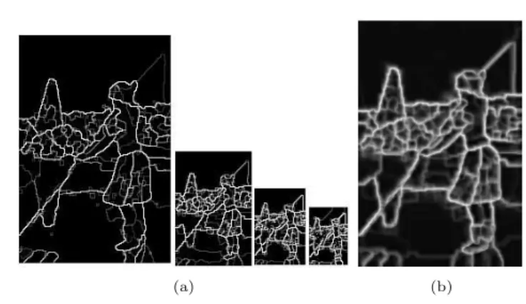
– Multi-scale representation by resampling: Given g, at each iteration i, the image g is resampled in a squared grid of size fixed : nj × nj. This resampling is done by selecting 50% of pixels in a nj× nj neighbourhood, which are used to estimate the mean value. The corresponding downsampled by averaging gradient is denoted g↓ji . The step is applied for S = 4 scales, such that n1= 2 × 2, n2= 4 × 4, n3= 6 × 6 and n4= 8 × 8. An example is illustrated in Fig. 3(d). We denote g↓0i = g.

– Multi-scale SW: For each realization i of resampled gradient, compute the SW at each scale j: PSW(g↓ji ), see example in Fig. 4.

(a) (b) (c) (d)

Fig. 3.(a) Example of image from the BSD [11], (b) corresponding ground truth [11], (c) the original Pb gradient, (d) a multi-scale representation based on sampling by mean value computation.

– Multiple realizations and bagging: Resampling procedure is iterated N times for each of the S scales. Bagging involves to combine all the pdf of contours. Note that an upsampling step, here we chose the bilinear interpo-lation, is required to combine at the original resolution. Thus, the bagging stochastic watershed is computed as

PBSW(g) = (SN )−1 N X i=1 S X j=0 wj h PSW(g↓ji ) i↑j . (3)

We have empirically fixed the following scale weights: w1 = 0.6, w2 = 0.2, w3 = 0.1, w4 = 0.1. The weights can be chosen according to the pattern spectrum of the image.

3.3 Improved accuracy of BSW

Before discussing the results, let us prove that by aggregating the different multi-scale replicates of SW the accuracy of this estimator is theoretically improved.

Let us write B = {b} the set of boundaries b of an image, and P (b) the true probability boundary of b ∈ B. Let us consider PSW(b ∈ B, g) the estimation of the probability boundary by means of the SW from gradient g, and PBSW(b ∈ B, g) the estimation using the BSW. We note by L = {g↓_{} the set of resampled} gradients where the SW is applied. Then, we have:

PBSW(b ∈ B, g) = EL[PSW(b ∈ B, g↓)]. (4) We define the quadratic error of estimation of the probability boundary on g↓ as:

EPSW = EB[P (b) − PSW(b ∈ B, g

↓

(a) (b)

Fig. 4.In (a) multiscale stochastic watershed for a given realization i of bagging, in (b) the result of the bagging stochastic watershed

The expectation of this error on L is given by ELEB[P (b) − PSW(b ∈ B, g↓)]2, which can be rewritten as

EB(P (b)2) − 2EB[P (b)EL[PSW(b ∈ B, g↓)]] + EB[EL[PSW(b ∈ B, g↓)]2]. Now, by using the fact that E(z2_{) ≥ (E(z))}2_{, we obtain:}

ELEB[P (b) − PSW(b ∈ B, g↓)]2≥ EB[P (b) − PBSW(b ∈ B, g)]2= EPBSW. (6)

Therefore, we note that the average error of PSW is higher than the error of PBSW. In conclusion, by aggregating the SW we decrease the error of estimation of the probability boundaries, but we also decrease the image resolution.

4

Results on BSD

Evaluation of the BSW has been done in the BSD, containing 200 natural im-ages and their ground truths (with contours manually segmented by 5 differ-ent subjects. We have compared the results of Pb and gPb from [4], a simple morphological color gradient (G) [1], the stochastic watershed (SW) [2], the im-proved stochastic watershed (ISW) as introduced in [5] and the proposed bagging stochastic watershed (BSW). We have also include a last result which corre-sponds to a pdf obtained by multiplying the BSW with the spectral probability gradient proposed also in [4], this combination is named the spectral bagging stochastic watershed (SBSW).

Since the result of the algorithm is an image of probability of contours, by selecting different thresholds, one has a totally different set of contours. Similarly to [4], at each level of the threshold, the F-measure is calculated: F -measure = (2×Precision×Recall)/(Precision+Recall), showing a tradeoff between precision and recall. The main advantage of the F-measure is that, contrary to the ROC curve, does not depend on the true negatives, which may turn the results to be

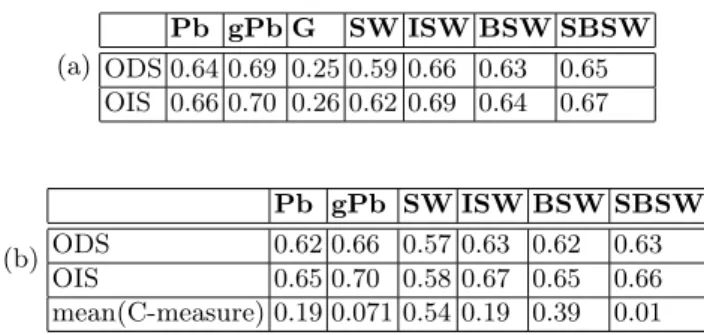
less discriminative. Table 1 summarizes the results for different methods. The curves of the F-measure are given in Fig. 5. As in [4], two features are computed from the F-measure: the ODS which is the optimal scale for the entire data set, and the OIS which is the optimal scale per image. We note the ISW and the here proposed BSW improves the results produced by the SW, with comparable performances. However, none of the morphological approaches are better than the gPb, which we remind is based on a learning procedure.

Thresholding and calculating F-measure of the pdf produce the optimal set of boundaries, but not the optimal regions. Instead of using a simple threshold on the pdf, we propose to compute a watershed transform after applying a h-reconstruction on the pdf. That produces a segmentation into closed regions and the choice of h is related to the contrast of probability. When this approach is obtained for different values of h we obtain a hierarchy of segmentations [13], related also to the so-called ultrametric contour map in [4]. Now, the F-measure can be computed at each value of the hierarchy h. In addition, we propose to compute the following contrast feature:

C-measure = (X h h × F -measure(Sh))/ X h h (7)

where Shis the set of closed contours obtained from the h-reconstruction water-shed. The C-measure 7 represents the fact that one does not know what is the optimal value h∗_{, so the C-measure, that we develop is a mean over different} val-ues of h. On Table 1.(b), for each algorithm we have computed the mean of the C-measures over the 200 images. As one can notice, using this feature, the BSW and the ISW seem to be the best compromise in terms of contrast/F-measure.

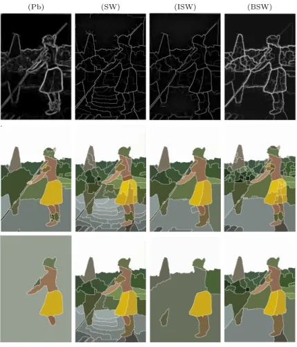
Fig. 6 provides also a comparison for the current image of the pdf of contours as well as two segmentations from each pdf, obtained by watershed combined with h-reconstruction (h = 0.1 and h = 0.25).

(a) Pb gPb G SW ISW BSW SBSW ODS 0.64 0.69 0.25 0.59 0.66 0.63 0.65 OIS 0.66 0.70 0.26 0.62 0.69 0.64 0.67 (b) Pb gPb SW ISW BSW SBSW ODS 0.62 0.66 0.57 0.63 0.62 0.63 OIS 0.65 0.70 0.58 0.67 0.65 0.66 mean(C-measure) 0.19 0.071 0.54 0.19 0.39 0.01

Table 1.(a) Comparison of F-measure (obtained by thresholding the pdf) on BSD. (b) Comparison of C-measure (obtained by hierarchy based on contrast) on BSD.

(a) (b)

Fig. 5.(a) F-measure of different algorithms, source of this plot [17] . (b) F-measure of algorithms compared on this paper.

5

Conclusion

Stochastic watershed is a probabilistic segmentation approach which can be inte-grated into a bagging paradigm to improve estimation of probability of contours. We have in particular considered a multi-scale approach of bagging stochastic watershed which at this point is fully unsupervised. In order to assess the per-formance in the BSD, we have used the F-measure and new criterion called the C-measure.

The combination of multi-scale bagging stochastic watershed with segmenta-tion learning architectures based for instance in convolusegmenta-tional networks should be considered in future research.

References

1. Angulo, J., & Serra, J. (2007). Modelling and Segmentation of Colour Images in Polar Representations. Image Vision and Computing, 25(4): 475–495.

2. Angulo, J., & Jeulin, D. (2007). Stochastic watershed segmentation. In Proc. of the 8th International Symposium on Mathematical Morphology (ISMM’2007), pp. 265–276, MCT/INPE.

3. Angulo, J., Velasco-Forero, S., & Chanussot, J. (2009.) Multiscale stochastic wa-tershed for unsupervised hyperspectral image segmentation. In Proc. of IEEE IGARSS’2009 (IEEE International Geoscience & Remote Sensing Symposium), Vol. III, 93–96.

4. Arbelaez, P., Maire, M., Fowlkes, C., & Malik, J. (2011). Contour detection and hierarchical image segmentation. IEEE Transactions on PAMI, 33(5): 898-916. 5. Bernander, K. B., Gustavsson, K., Selig, B., Sintorn, I. M., & Luengo Hendriks, C.

L. (2013). Improving the stochastic watershed. Pattern Recognition Letters, 34(9), 993-1000.

(Pb) (SW) (ISW) (BSW)

Fig. 6.First row, pdf of contours; second row, segmentation by keeping just the con-tours with more than 10% of contrast; third row, more than 25% of contrast. First column, Pb; second column, classical stochastic watershed (SW); third column, im-proved SW; fourth column bagging SW.

6. Beucher, S., & Lantu´ejoul, Ch. (1979). Use of watershed in contour detection. In Proc. of Int. Worshop Image Processing, Real-Time Edge and Motion Detec-tion/Estimation.

7. Breiman, L. (1996). Bagging predictors. Machine learning, 24(2):123–140.

8. LeCun, Y., & Bengio, Y. (1995). Convolutional networks for images, speech, and time series. The handbook of brain theory and neural networks, 3361.

9. L´opez-Mir, F., Naranjo, V., Morales, S., & Angulo, J. (2014). Probability Density Function of Object Contours Using Regional Regularized Stochastic Watershed. In Proc. IEEE ICIP’2014.

10. Malmberg, F., & Luengo Hendriks, C. L. (2014). An efficient algorithm for exact evaluation of stochastic watersheds. Pattern Recognition Letters, 47:80–84. 11. Martin, D., Fowlkes, C., Tal, D., & Malik, J. (2001). A database of human

seg-mented natural images and its application to evaluating segmentation algorithms and measuring ecological statistics. In Proc. of ICCV’01 (8th IEEE International Conference on Computer Vision), Vol. 2, pp. 416–423.

12. Meyer, F., Beucher, S. (2012). Morphological Segmentation. Journal of Mathemat-ical Imaging and Vision, 1(1):21–46.

13. Meyer, F. (2001). An overview of morphological segmentation. International Jour-nal of Pattern Recognition and Artificial Intelligence, 15(07), 1089–1118.

14. Meyer, F., & Stawiaski, J. (2010). A stochastic evaluation of the contour strength. In Proc. of DAGM’10, 513–522, Springer.

15. Meyer, F. (2015) Stochastic Watershed Hierarchies. In Proc. of ICAPR’15. 16. Roerdink, J.B.T.M., & Meijster, A. (2000) The Watershed Transform: Definitions,

Algorithms and Parallelization Strategies. Fundamenta Informaticae, 41(1-2):187– 228.