HAL Id: hal-00449995
https://hal.archives-ouvertes.fr/hal-00449995
Submitted on 24 Jan 2010
HAL is a multi-disciplinary open access
archive for the deposit and dissemination of
sci-entific research documents, whether they are
pub-lished or not. The documents may come from
teaching and research institutions in France or
abroad, or from public or private research centers.
L’archive ouverte pluridisciplinaire HAL, est
destinée au dépôt et à la diffusion de documents
scientifiques de niveau recherche, publiés ou non,
émanant des établissements d’enseignement et de
recherche français ou étrangers, des laboratoires
publics ou privés.
Optimization of Data Flow Computations using
Canonical TED Representation
Maciej Ciesielski, Jeremie Guillot, Daniel Gomez-Prado, Quian Ren,
Emmanuel Boutillon
To cite this version:
Maciej Ciesielski, Jeremie Guillot, Daniel Gomez-Prado, Quian Ren, Emmanuel Boutillon.
Optimiza-tion of Data Flow ComputaOptimiza-tions using Canonical TED RepresentaOptimiza-tion. IEEE Design & Test, IEEE,
2009, 26 (4), pp.46-57. �hal-00449995�
High-level Transformations using Canonical Dataflow Representation
M. Ciesielski, J. Guillot*, D. Gomez-Prado, Q. Ren, E. Boutillon*
ECE Dept., University of Massachusetts, Amherst, MA, USA
∗
Lab-STICC, Universit´e de Bretagne Sud, Lorient, France
1
Abstract
This paper describes a systematic method and an experi-mental software system for high-level transformations of de-signs specified at behavioral level. The goal is to transform the initial design specifications into an optimized data flow graph (DFG) better suited for high-level synthesis. The opti-mizing transformations are based on a canonical Taylor Ex-pansion Diagram (TED) representation, followed by struc-tural transformations of the resulting DFG network. The sys-tem is intended for data-flow and computation-intensive de-signs used in computer graphics and digital signal processing applications.
2
Introduction
A considerable progress has been made during the last two decades in behavioral and High-Level Synthesis (HLS), making it possible to synthesize designs specified using Hardware Description Languages (HDL) and C or C++ lan-guage. Those tools automatically generate a Register Trans-fer Level (RTL) specification of the circuit from a bit-accurate algorithm description for a given target technology and the application constraints (latency, throughput, preci-sion, etc.). The algorithmic description used as input to high-level synthesis does not require explicit timing information for all operations of the algorithm and thus provides a higher level of abstraction than the RTL model. Thanks to high-level synthesis, the designer can faster and more easily ex-plore different algorithmic solutions. An important produc-tivity leap is thus achieved.
However, the optimizations offered by the high-level syn-thesis tools are limited to algorithms for scheduling and re-source allocation performed on a fixed Data Flow Graph (DFG), derived directly from the initial HDL specification [1]. Modification of the DFG, if any, is provided by rewrit-ing the initial specification. In this sense the high-level syn-thesis flow remains “classical”: the algorithm is first de-fined and validated without any hardware constraints; a bit-accurate model is then derived to obtain an initial hardware specification of the design, which becomes input to the HLS flow. With this approach the quality of the final hardware implementation strongly depends on the quality of the hand-written hardware specification. In order to explore other so-lutions, the user needs to rewrite the original specification, from which another DFG is derived and synthesized.
Why not then relax the process and start the flow at the Algorithm level, where the design is given as an abstract specification, sufficient to generate the required architecture but without the detailed timing and hardware information. While this may not be possible for all the designs (in par-ticular control applications), data-intensive applications can benefit from this approach. For example, in signal processing applications that deal with noisy signals there may be several ways to perform the computation described by the algorithm. Some of them may lead to an acceptable hardware solution even if it introduces a moderate level of internal computation noise (SNR). In general, such a noise will not affect the per-formance of the system in a significant way, while the result-ing architecture may give a better hardware implementation in terms of circuit area, latency, or power.
To give a simple example, in fixed precision computa-tion, the expression A· B + A · C is not strictly equal to A(B + C) in terms of signal-to-noise ratio. Nonlinear op-erations of rounding, truncation and saturation, required to keep the internal precision fixed, are not applied in the two expressions in the same order; as a result, the two computa-tions may differ slightly. Nevertheless, in a common signal processing application, the two expressions can be consid-ered identical from the computational view point. The one with a better hardware cost can be selected for final hardware implementation. In this example, the expression A(B + C) may be chosen as it needs to schedule fewer operators, thus resulting in smaller latency and/or circuit area.
In this context, the road to automatic transformation of the design specification that preserves its intended “require-ment” is open. Such a specification transformation tool should allow the designer to express the specification rapidly and to rewrite it into a form that will optimize the final hard-ware implementation. Such a modification must take into consideration the specific design flow and the constraints of the application.
Automatic specification transformation is an old concept. In fact, software compilers commonly use such optimiza-tion techniques as dead code eliminaoptimiza-tion, constant propa-gation, common subexpression elimination, and others [2]. Some of those compilation techniques are also used by HLS tools. Several high-level synthesis systems, such as Cyber [3] and Spark [4], use different methods for code optimiza-tion (kernel-based algebraic factorizaoptimiza-tion, branch balancing, speculative code motion methods, dead code elimination, etc.) but without guaranteeing optimality of the high-level transformations. For example, very few of them, if any, are
F = A*B + A*C B C A 1 F A B A C t2 t1 A B A C t1 t2 t3 A B C t1 t2
c) 3 cycles, 1 Mpy, 1 Add d) 2 cycles, 1 Mpy, 1 Add b) 2 cycles, 2 Mpy, 1 Add
a) Canonical TED representation
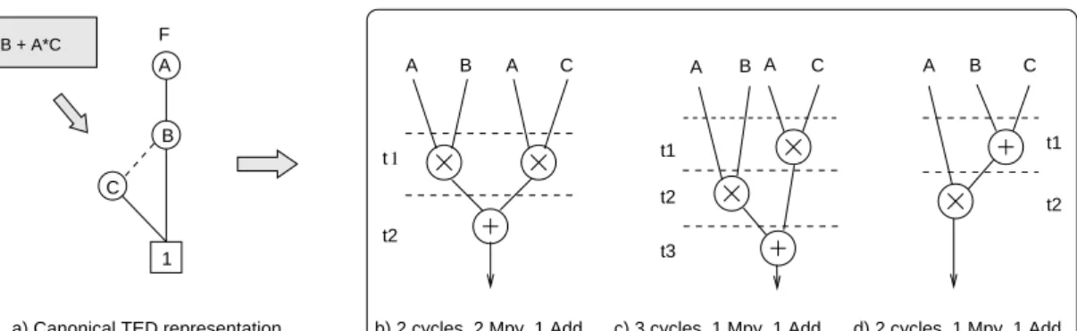
Figure 1. High-level transformations: a) Canonical TED representation; b),c,) DFGs corresponding to the original expressionF = A · B + A · C; d) DFG for the transformed expression,F= A · (B + C).
able to recognize that the expression X= (a+ b)(c+ d)− a· c−a·d−b·c−b·d trivially reduces to X = 0. With the excep-tion for a few specialized systems for DSP code generaexcep-tion, such as SPIRAL [5], these methods rely on simple manipu-lations of algebraic expressions based on term rewriting and basic algebraic properties (associativity, commutativity, and distributivity) that do not guarantee optimality.
This paper describes a systematic method for transform-ing an initial design specification into an optimized DFG, better suited for high-level synthesis. The optimizing trans-formations are based on a canonical, graph-based representa-tion, called Taylor Expansion Diagram (TED) [6]. The goal is to generate a DFG, which - when given as input to a stan-dard high-level synthesis tool - will produce the best hard-ware implementation in terms of latency and/or hardhard-ware cost.
To motivate the concept of high-level transformations supported by the canonical TED representation, consider a simple computation, F = A · B + A · C, where variables A, B, C are word-level signals. Figure 1(a) shows the canon-ical TED representation encoding this expression (discussed in the next section). Figures 1(b) and (c) show two possi-ble scheduled DFGs that can be obtained for this expression using any of the standard HLS tools. We should emphasize that both solutions are obtained from a fixed DFG, derived directly form the original expression. They have the same structure and differ only in the scheduling of the DFG opera-tions. The DFG in Figure 1(b) minimizes the design latency and requires one adder and two multipliers, while the one in Figure 1(c) reduces the number of assigned multipliers to one, at a cost of the increased latency.
Figure 1(d) shows a solution that can be obtained by trans-forming the original specification F = A · B + A · C into F = A · (B + C), which corresponds to a different DFG. This DFG requires only one adder and one multiplier and can be scheduled in two control steps, as shown in the figure. This implementation cannot be obtained from the initial DFG by simple structural transformation, and requires functional transformation (in this case factorization) of the original ex-pression which preserves its original behavior.
The remainder of the paper explains how such a transfor-mation and the optimization of the corresponding DFG can
be obtained using the canonical TED representation. These optimizing transformations are implemented in the soft-ware system, TDS, intended for data-flow and computation-intensive designs used in computer graphics and digital sig-nal processing applications. TDS system is available on line [7].
3
Taylor Expansion Diagrams (TED)
Taylor Expansion Diagram is a compact, word-level, graph-based data structure that provides an efficient way to represent computation in a canonical, factored form [6]. It is particularly suitable for algorithm-oriented applications, such as signal and image processing, with computations modeled as polynomial expressions.
A multi-variate polynomial expression, f(x, y, ...), can be represented using Taylor series expansion w.r.t. variable x around the origin x= 0 as follows:
f(x, y, . . .) = f (x = 0) + xf′ (0) +1 2x 2 f”(0) + . . . (1) where f′ (x = 0), f′′
(x = 0), etc, are the successive deriva-tives of f w.r.t. x, evaluated at x= 0. The individual terms of the expression, f(0), f′
(0), f ”(0), etc., are then decom-posed iteratively with respect to the remaining variables on which they depend (y, .., etc.), one variable at a time.
The resulting decomposition is stored as a directed acyclic graph, called Taylor Expansion Diagram (TED). Each node of the TED is labeled with the name of the variable at the current decomposition level and represents the expression rooted at this node. The top node of the TED represents the main function f(x, y, . . .), and is associated with the first de-composing variable, x. Each term of the expansion at a given decomposition level is represented as a directed edge from the current decomposition node to its respective derivative term, f(0), f′(0), f ”(0), etc. Each edge is labeled with the
weight, representing the coefficient of the respective term in the expression.
Most of the TEDs presented in this work are linear TEDs, representing linear multi-variate polynomials and containing only two types of edges: multiplicative (or linear) edges, resented in the TED as solid lines; and additive edges, rep-resented as dotted edges. Nonlinear expressions can be
ially converted into linear ones, by transforming each occur-rence of a nonlinear term xkinto a product x
1· · · xk, where
xi = xj. Such a transformed expression is then represented
as a linear TED.
The expression encoded in the TED graph is computed as a sum of the expressions of all the paths, from the TED root to terminal 1. An expression for each path is computed as a product of the edge expressions, each such an expression being a product of the variable in its respective power and the edge weight. Only non-trivial terms, corresponding to edges with non-zero weights, are stored in the graph.
As an example, consider an expression F = A · B + A · C represented by the TED in Figure 1(a). This expression is computed in the graph as a sum of two paths from TED root to terminal node 1: A· B and A · B0
· C = A · C. In fact, TED encodes such an expression in factored form, F = A · (B + C), since variable A is common to both paths. This is manifested in the graph by the presence of the subex-pression(B + C), rooted at node B, which can be factored out. This is an important feature of the TED representation, employed by TED-based factorization and common subex-pression extraction described in the remainder of the paper.
In summary, TED represents finite multi-variate polyno-mials and maps word-level inputs into word-level outputs. TED is reduced and normalized in a similar way as BDDs [8] and BMDs [9]. Finally, the reduced, normalized and or-dered TED is canonical for a given variable order. Detailed description of the TED representation and its application to verification can be found in [6].
4
TED-based Decomposition
The principal goal of algebraic factorization and decom-position is to minimize the number of arithmetic operations (additions and multiplications) in the expression. A simple example of factorization is the transformation of the expres-sion F = AB + AC into F = A(B + C), referred to in Figure 1, which reduces the number of multiplications from two to one. If a sub-expression appears more than once in the expression, it can be extracted and replaced by a new vari-able, which reduces the overall complexity of an expression and its hardware implementation. This process is known as
common subexpression elimination (CSE). Simplification of
an expression (or of a set of expressions) by means of factor-ization and CSE is commonly referred to as decomposition.
Decomposition of algebraic expressions can be performed directly on the TED graph. As mentioned earlier, TED al-ready encodes the expression in a compact, factored form. The goal of TED decomposition is to find a factored form that will produce a DFG with minimum hardware cost of the final, scheduled implementation. This is in contrast to a straightforward minimization of the number of operations in an unscheduled DFG, that has been the subject of all the known previous approaches [10, 11].
This section describes two methods for TED decomposi-tion. One is based on the factorization and common subex-pression extraction performed on a TED with a given vari-able order, without modifying that order. This method is ap-plicable to generic expressions, without any particular
struc-ture. The other method is a dynamic CSE, where common subexpressions are derived by dynamically modifying TED variable order in a systematic way. This method is partic-ularly suitable for well-structured DSP transforms, such as DCT, DFT, WHT, etc, where they can discover common computing patterns, such as butterfly.
4.1
Static TED Decomposition
The static TED decomposition approach extends the orig-inal cut-based decomposition method of Askar [10]. Basic idea of the cut-based decomposition is to identify in the TED a set of cuts, i.e., additive edges and multiplicative nodes (called dominators) whose removal separates the graph into two disjoint subgraphs, Each time an additive or multiplica-tive cut is applied to a TED, a hardware operator (ADD or
MULT) is introduced in the DFG to perform the required op-eration on the two subexpressions. This way, a functional TED representation, is eventually transformed into a
struc-tural data flow graph (DFG) representation. It has been
shown that different cut sequences generate different DFGs, from which the DFG with best property (typically latency) can be chosen.
By construction, the cut-based decomposition method is limited to a disjoint decomposition. Many TEDs, however, such as the one shown in Figure 2(a), do not have a disjoint decomposition property and must be handled differently.
The decomposition described here applies to an arbitrary TED graph (linearized, if necessary), with both disjoint and non-disjoint decomposition. The TED decomposition is ap-plied in a bottom-up fashion by iteratively extracting com-mon terms (sums and products of variables) and replacing them with new variables. The method is based on a series of functional transformations that decompose the TED graph into a set of irreducible TEDs, from which a final DFG repre-sentation is constructed. The decomposition is guided by the quality of the resulting scheduled DFG (measured in terms of its latency or resource utilization) and not by the number of operators in an unscheduled DFG.
The basic procedure of the TED decomposition is the sub operation, which extracts a subexpression expr from the TED and substitutes it with a new variable var. First, the variables in the expression expr are pushed to the bottom of the TED, respecting the relative order of variables in the expression. Let the top-most variable in expr be v. Assuming that expr is contained in the original TED, this expression will appear in the reordered TED as a subgraph rooted at node v. The extraction of expr is accomplished by removing the subgraph rooted at v and connecting the reference edge(s) to terminal node 1.
The extraction operation is shown in Figure 2(a,b), where subexpression expr = (c + d) is extracted from F = (a + b)(c + d) + d. If an internal portion of the extracted subexpression is used by other portions of the TED, i.e., if any of the internal subgraph nodes is referenced by the TED at nodes different than its top node v, that portion of expr is automatically duplicated before extraction and variable sub-stitution. This is also visible in Figure 2(b), with node d being duplicated in the process.
TED decomposition is performed in a bottom-up manner, by extracting simpler terms and replacing them with new variables (nodes), followed by a similar decomposition of the resulting top-level level graph. The final result of the decomposition is a series of irreducible TEDs, related hierar-chically. Specifically, the decomposing algorithm identifies and extracts sum-terms and product terms in the TED and substitutes them by new variables, using the sub operation described above. Computational complexity of the extrac-tion algorithms is polynomial in the number of TED nodes. Each new term constitutes an irreducible TED graph, which is then translated directly into a DFG composed of the op-erators of one type (adders for sum-term, and multipliers for product term).
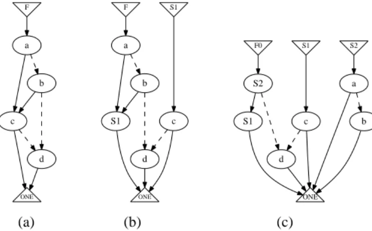
The TED decomposition and DFG construction is illus-trated with a simple example in Figure 2. This TED does not have a single additive cut edge that would separate the graph disjunctively into two disjoint subgraphs; neither does it have a dominator node that would decompose it conjunctively into disjoint subgraphs, and hence cannot be decomposed using cut-based method. The decomposition starts with identifying and extracting expression S1= c + d, followed by extracting
S2 = a + b, represented as an irreducible TED. Note that
term d is automatically duplicated in this procedure.
F a b c d ONE F a S1 b S1 c ONE d F0 S2 S1 d S1 c ONE S2 a b (a) (b) (c)
Figure 2.Static TED decomposition; (a) Original TED for expression F0= ac + bc + ad + bd: (b) TED after extracting
S1 = c + d; (c) Final TED after extracting S2 = a + b,
resulting in Normal Factored Form F0= (a+b)·(c+d)+d.
Product terms can be identified in the TED as a set of nodes connected by multiplicative edges, such that the inter-mediate nodes in the series do not have any additive incom-ing or outgoincom-ing edges. Only the startincom-ing and endincom-ing nodes can have incident additive edges. In Fig. 2(a) no product terms can be found at this decomposition level. A sum term appears in the TED graph as a set of variables, connected by multiplicative edges to a common node and linked together by additive edges. In Fig. 2(a) two such sum-terms can be identified and extracted as reducible TEDs: S1 = c + d and
S2 = a + b. Each irreducible subgraph is then replaced by
a single node in the original TED to produce TED shown in Fig. 2(c). This procedure is repeated iteratively until the TED is reduced to the simplest, irreducible form. The re-sulting TED is then subjected to the final decomposition us-ing the fundamental Taylor expansion procedure. The graph is traversed in a topological order, starting at the root node.
At each visited node v the expression F(v) is computed as F(v) = F0+ v · F1, where F0is the function rooted at the
first node reached from v by an additive edge, and F1is the
function rooted at the first node reached from v by a multi-plicative edge. Using this procedure, the TED in Figure 2(c) produces the decomposed expression F = S2· S1+ d, where
S1= c + d and S2= a + b.
4.2
Dynamic TED Factorization
An alternative approach to TED decomposition is based on the dynamic factorization and common subexpression elimination (CSE). This approach is illustrated with an exam-ple of the Discrete Cosine Transform (DCT), used frequently in multimedia applications. The DCT of type 2 is defined as
Y(j) = N −1 X k=0 xkcos[ π Nj(k + 1 2)], k = 0, 1, 2, ..., N − 1 and computed by the following algorithm:
for (j = 0; j < N ; j++) { tmp = 0;
for (k = 0; k< N ; k++)
tmp+=x[k]*cos(pi*j*(k+0.5)/N); y[j] = tmp; }
It can be represented in a matrix form as y = M · x, where x and y are the input and output vectors, and M is the transform matrix composed of the cosine terms, eq. (2).
M =
cos(0) cos(0) cos(0) cos(0) cos(π 8) cos( 3π 8) cos( 5π 8) cos( 7π 8 ) cos(π 4) cos( 3π 4) cos(5 π 4) cos(7 π 4) cos(3π 8 ) cos( 7π 8) cos( π 8) cos( 5π 8 ) = A A A A B C −C −B D −D −D D C −B B −C (2)
In its direct form the computation involves 16 multipli-cations and 12 additions. However, by recognizing the de-pendence between the cosine terms it is possible to express the matrix using symbolic coefficients, as shown in the above equation. The coefficients with the same numeric value are represented by the same symbolic variable. The matrix M for the DCT example has four distinct coefficients, A, B, C, and D (for simplicity, we neglect the fact that A= cos(0) = 1). This representation makes it possible to factorize the ex-pressions and subsequently reduce the number of operations to 6 multiplications and 8 additions, as shown by the equa-tions (3). This simplification can be achieved by extracting subexpressions(x0+x3), (x0−x3), (x1+x2), and (x1−x2),
shared between the respective outputs, and substituting them with new variables.
y0= A · ((x0+ x3) + (x1+ x2))
y1= B · (x0− x3) + C · (x1− x2)
y2= D · ((x0+ x3) − (x1+ x2))
y3= C · (x0− x3) − B · (x1− x2) (3)
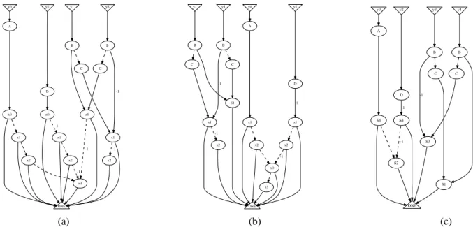
The initial TED representation for the DCT matrix in eq. (2) is shown in Figure 3(a). The subsequent parts of the fig-ure show the transformation of the TED that produces the above factorization.
The key to obtaining efficient TED-based factorization and common subexpression extraction (CSE) for this class of DSP design is to represent the coefficients of the matrix expressions as variables and to place them on top of the TED graph. This is in contrast to a traditional TED representa-tion, where constants are represented as labels on the graph edges. In the case of the DCT transform, the coefficients A, B, C, D are treated as symbolic variables and placed on top of the TED, as shown in Figure 3(a).
The candidate expressions for factorization in such a TED are obtained by identifying the nodes with multiple parent (reference) edges. The subexpression rooted at such nodes are extracted from the graph and replaced by new variables.
The TED in Figure 3(a) exposes two subexpressions for possible extraction: 1) the rightmost node associated with variable x0 (show in red), the root of subexpression(x0−
x3); and 2) the rightmost node associated with variable x1
(pointed to by nodes C, B), which is the root of subexpres-sion(x1− x2). The first expressions is extracted from the
graph and substituted with a new variable, S1 = (x0− x3).
Variable S1 is then pushed to the top of the diagram, below constant nodes, as shown in Figure 3(b). This new structure exposes another expression to be extracted, namely S2 = (x0+ x3). Once the subexpression is extracted, variable S2
is also pushed up. The next iterations of the algorithm leads to substitutions S3 = (x1− x2) and S4 = (x1+ x2),
re-sulting in a final TED shown in Figure 3(c). At this point there are no more original variables that can be pushed to the top, and the algorithm terminates. As a result, the above TED-based common subexpression elimination results in the following expressions: y0= A · (S2 + S4), y1 = B · S1 + C · S3 y2 = D · (S2 − S4), y3 = C · S1 − B · S3, where: S1 = (x0 − x3), S2 = (x0 + x3), S3 = (x1 − x2) and S4 = (x1 + x2).
Considering that A = 1, the computation of such opti-mized expressions requires only 5 multiplications and 8 ad-ditions, a significant reduction from the 16 multiplications and 12 additions of the initial expressions.
5
DFG Generation and Optimization
The TED decomposition procedures described in the pre-vious section produce simplified algebraic expressions in factored form. Each addition operation in the expression cor-responds to an additive edge of some irreducible TED, and each multiplication corresponds to a multiplicative edge in an irreducible TED, obtained from the TED decomposition. We refer to such a form as Normal Factor Form (NFF) of the TED.
It can be shown that normal factored form is minimal and unique for a given TED with fixed variable ordering. The
form is minimal in the sense that it requires minimum num-ber of operators of each type (adders and multipliers) to de-scribe the algebraic expression encoded in the TED. No other expression that can be derived from this TED (with the given variable order) can have fewer operations. For example, the NFF for the TED in Fig. 1 is F = A·(B + C), with oneADD
and oneMULToperator. Other forms, such as AB + AC, have two multiply operators, which are not present in this graph (the multiplicative edges leading to the terminal node 1 represent trivial multiplications by 1 and do not count). Such a form is also unique, if the order of variables in the normal factored form is compatible with that in the TED. In the above example, the forms A(C + B) or (B + C)A are not NFFs, since the variable order in those expressions is not compatible with that in the TED in Fig. 1(a).
The concept of normal factored form can be further clar-ified with the TED in Fig. 2. The normal factored form for this TED is F0 = (a + b) · (c + d) + d. It contains three
adders, corresponding to the three additive edges in the ir-reducible TEDs, S1, S2, and the top-level TED, F0, shown
in Fig. 2(c); and one multiplier corresponding to the multi-plicative edge in the TED for F0, in Fig. 2(c). This is the
minimum number of operators that can be obtained for the TED with the variable order{a, b, c, d}. The form is unique, since the ordering of variables in each term is compatible with the ordering of variables in the TED.
It should be obvious from the above discussion that the NFF for a given TED depends only on the structure of the ini-tial TED and the ordering of its variables. Hence, a TED vari-able ordering plays a central role in deriving decompositions that will lead to efficient hardware implementations. Several variable ordering algorithms have been developed for this purpose, including static ordering and dynamic re-ordering schemes, similar to those in BDDs. However, TED ordering is driven by the complexity of the NFF and the structure of the resulting DFGs, rather than by the number of TED nodes.
5.1
Data Flow Graph Generation
Once the algebraic expression represented by TED has been decomposed, a structural DFG representation of the optimized expression is obtained by replacing the algebraic operations in the normal factored form into hardware oper-ators of the DFG. However, unlike Normal Factored Form, the DFG representation is not unique. While the number of operators remains fixed (dictated by the ordered TED), the DFG can be further restructured and balanced to mini-mize its latency. In addition to replacing operator chains by logarithmic trees, standard logic synthesis methods, such as collapsing and re-decomposition, taking into consideration signal arrival times can be used for this purpose [1].
An important feature of the TED decomposition, con-cluded by the generation of an optimized DFG, is that it has insight into the final DFG structure. Different DFG solu-tions can be generated by modifying the TED variable or-der, performing static and dynamic factorization, followed by a fast generation of the minimum-latency DFG. This ap-proach makes it possible to minimize the hardware resources or latency in the final, scheduled implementation, not just
y0 A y1 B y2 D y3 B ONE x0 C x0 C x1 -1 x0 x1 x3 -1 x1 -1 x2 x2 -1 x2 -1 y0 A y1 B y2 D y3 B ONE x1 C S1 C x1 -1 x1 -1 x2 x2 -1 x2 x0 -1 x3 y0 A y1 B y2 D y3 B ONE S4 C S1 C S3 -1 S4 -1 S2 -1 (a) (b) (c)
Figure 3. a) Initial TED of DCT2-4, b) TED after extracting S1= (x0− x3); c) final TED after extracting S2= (x0+ x3), S3=
(x1− x2) and S4= (x1+ x2), resulting in the final factored form of the transform.
the number of operations in the DFG graph. The solution that meets the required objective is selected.
In summary, TED variable ordering, static and dynamic factorization/CSE, and DFG restructuring, are at the core of the optimization techniques employed by TED decomposi-tion.
5.2
Replacing Multipliers by Shifters
Multiplications by constants are common in designs in-volving linear systems, especially in computation intensive applications such as DSP. It is well known that multipli-cations by integers can be implemented more efficiently in hardware by converting them into a sequence of shifts and additions or subtractions. Standard techniques are available to perform such a transformation based on Canonical Signed Digit (CSD) representation. However, these methods do not address common subexpression elimination or factorization involving shifters. In this section we present a systematic way to transform integer multiplications into shifters using the TED structure. This is done by introducing a special ‘left
shift’ variable L into the TED, while maintaining its
canonic-ity. The modified TED can then be decomposed using meth-ods described earlier.
First, each integer constant C is represented in the CSD format as C=P
i(ki· 2i), where ki∈ (−1, 0, 1). By
intro-ducing a new variable L to replace constant 2, C can be rep-resented asP
i(ki· L
i). The term Liin this expression
rep-resents left shift by i bits. The TED with the shift variables is then subjected to a regular TED decomposition. Finally, in the DFG generated by the TED decomposition the terms involving shift variables, Lk, are replaced by k-bit shifters.
The example in Figure 4 illustrates this procedure for the expression F = 7a + 6b. The original TED is shown in
Figure 4(a) and the corresponding DFG with constant mul-tipliers in Figure 4(b). The original expression is trans-formed into an expression with the shift variable L: F = (L3− 1) · a + (L3− L1) · b = L3· (a + b) − (a + L · b), and
represented by a non-linear TED shown in Figure 4(c). Each edge of the TED is labeled with a pair(∧p, w), where∧
p rep-resents the power of variable (stored as the node label), and w represents the edge weight (multiplicative constant) asso-ciated with this term. For example, the edge labeled(∧3, 1)
coming out of variable L represents a non-linear term L3· 1.
The TED subgraph rooted at the right node, labeled a, rep-resents expression a+ b. The dotted between nodes a and b, labeled(∧
0, 1), simply represents an addition.
The modified TED is then transformed into a DFG, where multiplications with inputs Lkare replaced by k-bit shifters, as shown in Figure 4(d). The optimized expression corre-sponding to this DFG is F = ((a + b) << 2 − b) << 1 − a, where the symbol “<< k” refers to left shift by k bits. This implementation requires only three adders/subtracters and two shifters, a considerable gain compared to the two multi-plications and one addition needed to implement the original expression.
6
TDS System
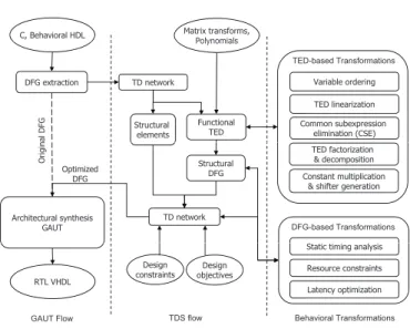
The TED decomposition described here was implemented as part of a prototype system, TDS, shown in Fig. 5. The input to the system is the design specified in C/C++, behav-ioral HDL, or given in form or a DSP matrix. The system can also internally generate matrices for some of the stan-dard linear DSP transforms, such as DCT, DFT, WHT, etc., to be used as input. The left part of the figure shows the tra-ditional high-level synthesis flow, which extracts the control data flow (CDFG) from the initial specification and performs standard high-level synthesis operations: scheduling,
F0 a 1 b ^0 6 ONE ^1 7 ^1 1 F0 + a * 7 b * 6 (a) (b) F0 L 1 a ^0 -1 b ^1 -1 a ^3 1 ONE ^1 1 ^1 1 ^0 1 ^1 1 F0 -a + + b << << 3 1 (c) (d)
Figure 4. Replacing constant multiplications by shift op-erations: (a) Original TED for F0 = 7a + 6b; (b) Initial
DFG with constant multipliers; (c) TED after introducing
shift variable L; (d) Final DFG with shifters, corresponding
to the expression F = ((a + b) << 2 − b) << 1 − a.
tion and resource binding. The right part of the figure shows the actual TDS optimization flow. It transforms the data flow graph extracted from the initial specification into an opti-mized DFG using a host of TED-based decomposition and DFG optimization techniques, and passes the modified DFG to a high-level synthesis tool. Currently, an academic syn-thesis tool, GAUT [12], is used for front-end parsing and for the final high level synthesis, but any of the existing HLS tools can be used for this purpose (provided that compatible format interfaces are available).
The DFG extracted from the initial specification is trans-lated into a hybrid network composed of islands of functional blocks, represented using TEDs, and other operators (“struc-tural” elements). Specifically, TEDs are constructed from polynomial expressions that have finite Taylor expansion, de-scribing arithmetic components of the design (adders, mul-tipliers, multiplexers) as well as “if-then-else” statements. Those operators that cannot be represented as functional TEDs (such as comparators, saturators, etc.), are considered as black boxes in the hybrid network.
TDS optimizes the resulting hybrid TED/DFG network and transforms it into a final DFG using TED- and DFG-related optimizations. The entire DFG network is finally re-structured to minimize the latency. The system provides a set of interactive commands and optimization scripts that in-clude: variable ordering, TED linearization, static and dy-namic factorization, decomposition, replacement of constant
C, Behavioral HDL Matrix transforms,
Polynomials Variable ordering TED-based Transformations DFG extraction TD network Polynomials TED linearization Common subexpression elimination (CSE) n a l D F G Structural elements Functional TED TED factorization & decomposition Constant multiplication
& shifter generation Optimized DFG O ri g in Structural DFG DFG-based Transformations Architectural synthesis GAUT TD network
Static timing analysis
Latency optimization Resource constraints RTL VHDL Design objectives Design constraints y p Behavioral Transformations
GAUT Flow TDS flow
Figure 5.TDS system flow.
multiplications by shifters, DFG construction, balancing, etc.
7
Experimental Results
The system was tested on a number of practical designs from computer graphics applications, filters and DSP de-signs. Table 1 compares the implementation of a quintic
spline filter using: 1) the original design written in C; 2) the
design produced by CSE decomposition system of [11]; 3) and the design produced by TDS. All DFGs were synthe-sized using GAUT. The top row of the table reports the num-ber of arithmetic operations (adders, multipliers, shifters, subtractors) for unscheduled DFG. The remaining rows list the actual number of resources used for a given latency in the scheduled DFG; and the implementation area using GAUT (datapath only). Minimum latency for each solution are shown in bold. The results for circuits that cannot be synthesized for a given latency are marked with ’–’ (over-constrained).
Design Original CSE TDS
design solution solution Latency
+,×,≪,− Area +,×,≪,− Area +,×,≪,− Area (ns) Q u in ti c S p li n e DFG → 5,28,2,0 5,13,3,0 6,14,4,0 L=110 – – – – 1,5,1,0 460 L=120 – – – – 2,4,2,0 422 L=130 – – – – 1,4,1,0 377 L=140 – – 1,4,1,0 377 1,3,1,0 294 L=150 – – 1,3,1,0 294 1,3,1,0 294 L=160 – – 1,3,1,0 211 1,3,1,0 294 L=170 – – 1,2,1,0 211 1,3,1,0 294 L=180 1,5,1,0 460 1,2,1,0 211 1,2,1,0 211
Table 1. Quintic Spline achivable latency and area for different designs. The area reported is for GAUT.
As seen in the table the CSE solution has the smallest number of operations in the unscheduled DFG, and the la-tency of 140 ns. The lala-tency of DFG obtained by TDS was 110 ns, i.e., 21.4% faster, even though it had more DFG oper-ations. And for the minimum latency of 140 ns, obtained by CSE, TDS produced circuit implementation with area 22% smaller than CSE. Similar behavior has been observed for
all the tested designs. In all cases the latency of DFGs pro-duced by TDS was smaller; and (with an exception for Quar-tic Spline design), all of them also had smaller hardware area for the minimum latency produced by CSE.
Design
TDS vs
Original CSE
Latency (%) Area (%) Latency (%) Area (%) SG Filter 25.00 27.62 0.00 20.73 Cosine 38.88 50.42 8.33 9.45 Chrome 9.09 0.00 9.09 11.86 Chebyshev 41.17 48.68 16.66 15.23 Quintic 38.88 54.13 21.42 22.02 Quartic 37.50 30.50 23.07 -28.23 VCI 4x4 0.00 42.98 30.00 2.40 Average 27.22 36.33 15.51 7.64
Table 2. Percentage improvement of TDS vs Original and CSE on achievable latency; and area at the minimum achievable latency.
Table 2 summarizes the implementation results for these benchmarks. We can see that the implementations obtained by TDS have latency that is on average 15.5% smaller than that of CSE, and 27.2% smaller than the original DFGs. The hardware area of the TDS solutions for the reference latency (defined as the minimum latency obtained by the other two methods), is on average 7.6% smaller than that of CSE, and 36.3% smaller than the original design, without any DFG modification. These are significant improvements.
8
Conclusions
A new approach to the optimization of initial specifica-tion of data flow designs have been implemented that yields DFGs better suited for high-level synthesis and produces bet-ter hardware implementations than currently available. The TED-based optimization system guides the algebraic decom-position to obtain solutions with minimum latency and/or with minimum cost of operators in a scheduled DFG. The op-timized DFGs produce designs with lower latency than those obtained by a straightforward minimization of the number of arithmetic operations in the expression; and for the minimum latency obtained by the other methods, the generated designs require on average smaller hardware area.
The TDS system, developed as part of this research, goes beyond simple algebraic decomposition. It allows to handle arbitrary data-flow designs and algorithms written in C/C++ to optimized their data flow graphs prior to high-level synthesis. While currently the TDS system is integrated with an academic high-level synthesis tool, GAUT, we believe that it could be successfully used as a pre-compilation step in a commercial synthesis software, such as Catapult C. In this case, the optimized DFGs can be translated back into C (while preserving the optimized structure), and used as input to HLS, instead of the original DFGs. Finally, to turn TDS into a commercial-quality system, the issue of finite precision of the operators needs to be addressed. This is a subject of an ongoing work.
ACKNOWLEDGMENTS
This work was supported in part by the National Science Foundation, award No. CCF-0702506, and in part by CNRS, contract PICS 3053.
References
[1] G. DeMicheli, Synthesis and Optimization of Digital
Circuits, McGraw-Hill, 94.
[2] J.D. Ullman, Computational Aspects of VLSI, Com-puter Science Press, Rockville, Maryland, 1983. [3] K. Wakabayashi, Cyber: High Level Synthesis System
from Software into ASIC, pp. 127–151, Kluwer
Aca-demic Publishers, 1991.
[4] S. Gupta, R.K. Gupta, N.D. Dutt, and A. Nicolau,
SPARK: A Parallelizing Approach to the High-Level Synthesis of Digital Circuits, Kluwer Academic
Pub-lishers, 2004.
[5] M. P¨uschel, J.M.F. Moura, J. Johnson, D. Padua, M. Veloso, B.W. Singer, J. Xiong, F. Franchetti, A. Gaˇci´c, Y. Voronenko, K. Chen, R.W. Johnson, and N. Rizzolo, “SPIRAL: Code Generation for DSP Transforms”, Proceedings of the IEEE, vol. 93, no. 2, 2005.
[6] M. Ciesielski, P. Kalla, and S. Askar, “Taylor Expan-sion Diagrams: A Canonical Representation for Verifi-cation of Data Flow Designs”, IEEE Trans. on
Com-puters, vol. 55, no. 9, pp. 1188–1201, Sept. 2006.
[7] M. Ciesielski, D. Gomez-Prado, and Q. Ren, “TDS - Taylor Decomposition System.”, http://incascout.ecs.umass.edu/tds.
[8] A. Narayan and et al., “Partitioned ROBDDs: A Compact Canonical and Efficient Representation for Boolean Functions”, in Proc. ICCAD, ’96.
[9] R. E. Bryant and Y-A. Chen, “Verification of Arith-metic Functions with Binary Moment Diagrams”, in
Proc. Design Automation Conference, 1995, pp. 535–
541.
[10] M. Ciesielski, S Askar, D. Gomez-Prado, J. Guillot, and E. Boutillon, “Data-Flow Transformations using Taylor Expansion Diagrams”, in Design Automation and Test
in Europe, 2007, pp. 455–460.
[11] A. Hosangadi, F. Fallah, and R. Kastner, “Optimiz-ing Polynomial Expressions by Algebraic Factorization and Common Subexpression Elimination”, in IEEE
Transactions on CAD, Oct 2005, vol. 25, pp. 2012–
2022.
[12] Universit´e de Bretagne Sud Lab-STICC, “GAUT, Architectural Synthesis Tool”, http://http://www-labsticc.univ-ubs.fr/www-gaut/, 2008.