HAL Id: tel-01962957
https://tel.archives-ouvertes.fr/tel-01962957
Submitted on 21 Dec 2018
HAL is a multi-disciplinary open access
archive for the deposit and dissemination of sci-entific research documents, whether they are pub-lished or not. The documents may come from teaching and research institutions in France or abroad, or from public or private research centers.
L’archive ouverte pluridisciplinaire HAL, est destinée au dépôt et à la diffusion de documents scientifiques de niveau recherche, publiés ou non, émanant des établissements d’enseignement et de recherche français ou étrangers, des laboratoires publics ou privés.
Functional description of sequence constraints and
synthesis of combinatorial objects
Ekaterina Arafailova
To cite this version:
Ekaterina Arafailova. Functional description of sequence constraints and synthesis of combinatorial objects. Discrete Mathematics [cs.DM]. Ecole nationale supérieure Mines-Télécom Atlantique, 2018. English. �NNT : 2018IMTA0089�. �tel-01962957�
THÈSE DE DOCTORAT DE
L’École Nationale Supérieure Mines-Télécom Atlantique Bretagne Pays de la Loire – IMT Atlantique
COMUE UNIVERSITE BRETAGNE LOIRE
Ecole Doctorale N°601
Mathèmatique et Sciences et Technologies de l’Information et de la Communication Spécialité : Informatique et applications
Par
« Ekaterina ARAFAILOVA »
« Functional Description of Sequence Constraints and
Synthesis of Combinatorial Objects »
Thèse présentée et soutenue à IMT ATLANTIQUE, NANTES, le 25 septembre 2018
Unité de recherche : Laboratoire des Sciences du Numérique de Nantes (LS2N) Thèse N°: 2018IMTA0089
Rapporteurs avant soutenance :
Mme Michela Milano, Professeure, Università di Bologna M. Stanislav Živný, Associate Professor, University of Oxford
Composition du jury :
Président : M. Claude Jard, Professeur, Université de Nantes Examinateurs : M. John Hooker, Professeur, Carnegie Mellon University
Mme Michela Milano, Professeure, Università di Bologna M. Stanislav Živný, Associate Professor, University of Oxford Dir. de thèse : M. Nicolas Beldiceanu, Professeur, IMT Atlantique
2
Abstract
Contrary to the standard approach consisting in introducing ad hoc constraints and designing dedicated algorithms for handling their combinatorial aspect, this thesis takes another point of view. On the one hand, it focusses on describing a family of sequence constraints in a compositional way by multiple layers of functions. On the other hand, it addresses the combinatorial aspect of both a single constraint and a conjunction of such constraints by synthesising compositional combinatorial objects, namely bounds, linear inequalities, non-linear constraints and finite automata. These objects are obtained in a systematic way and are not instance-specific: they are parameterised by one or several constraints, by the number of variables in a considered sequence of variables, and by the initial domains of the variables. When synthesising such objects we draw full benefit both from the declarative view of such constraints, based on regular expressions, and from the operational view, based on finite transducers and register automata. There are many advantages of synthesising combinatorial objects rather than designing dedicated algorithms: 1) parameterised formulae can be applied in the context of several resolution techniques such as constraint programming or linear programming, whereas algorithms are typically tailored to a specific technique; 2) combinatorial objects can be combined together to provide better performance in practice; 3) finally, the quantities computed by some formulae can not just be used in an optimisation setting, but also in the context of data mining.
Key Words: constraint programming, automata, transducers, regular expressions, time series, parame-terised combinatorial objects, linear and non-linear invariants
3
Résumé
À l’opposé de l’approche consistant à concevoir au cas par cas des contraintes et des algorithmes leur étant dédiés, l’objet de cette thèse concerne d’une part la description de familles de contraintes en termes de composition de fonctions, et d’autre part la synthèse d’objets combinatoires pour de telles contraintes. Les objets concernés sont des bornes précises, des coupes linéaires, des invariants non-linéaires et des au-tomates finis; leur but principal est de prendre en compte l’aspect combinatoire d’une seule contrainte ou d’une conjonction de contraintes. Ces objets sont obtenus d’une façon systématique et sont paramétrés par une ou plusieurs contraintes, par le nombre de variables dans une séquence, et par les domaines initiaux de ces variables. Cela nous permet d’obtenir des objets indépendants d’une instance considérée. Afin de synthétiser des objets combinatoires nous tirons partie de la vue declarative de telles contraintes, basée sur les expressions régulières, ansi que la vue opérationnelle, basée sur les automates à registres et les trans-ducteurs finis. Il y a plusieurs avantages à synthétiser des objets combinatoires par rapport à la conception d’algorithmes dédiés: 1) on peut utiliser ces formules paramétrées dans plusieurs contextes, y compris la programmation par contraintes et la programmation linéaire, ce qui est beaucoup plus difficile avec des al-gorithmes; 2) la synergie entre des objets combinatoires nous donne une meilleure performance en pratique; 3) les quantités calculées par certaines des formules peuvent être utilisées non seulement dans le contexte de l’optimisation mais aussi pour la fouille de données.
Mots clés: programmation par contraintes, automates, transducteurs, expressions régulières, séries tem-porelles, objets combinatoires paramétrés, invariants linéaires et non-linéaires
4
Acknowledgements
First of all, I would like to thank my thesis director Nicolas Beldiceanu. Thank you for your support during these three years, the knowledge and the experience that you have handed over to me, for your precious advice about many things. It was a great honour and a pleasure to work with you for three years.
I would like to thank my co-director Rémi Douence. Thank you for your feedback on my writing and presentations, for sharing your opinion about our work, and for bringing a different point of view in what we were doing.
I would like to thank my jury members: Michela Milano, Stanislav Živný, John Hooker and Claude Jard. Thank you very much for reviewing and examining my work and for your valuable feedback.
I would like to thank the EU H2020 programme under grant 640954 for the GRACeFUL project for funding my thesis and everyone with whom I had an opportunity to work with during the project.
I would like to thank Helmut Simonis with whom I had an opportunity to co-author all my papers. Thank you for sharing your knowledge about the practical side of our work, for showing Cork, for interesting discussions on various topics, and for the delicious biscuits.
I would like to thank my other co-authors, Mats Carlsson, Pierre Flener, María Andreína Francisco Rodríguez, and Justin Pearson. Thank you for all pleasure and fun I had when working with you, for the picnics and the barbecues, and for your warm welcome in Uppsala.
I would like to thank the members of the TASC research group: Amine Balafrej, Anicet Bart, Philippe David, Arthur Godet, Giovanni Lo Bianco, Xavier Lorca, Gilles Madi Wamba, Thierry Petit, Charles Prud’homme, Gilles Simonin, and Charlotte Truchet. Thank you for all the laughter and interesting discus-sions that we had during coffee breaks.
I would like to thank Catherine Fourny, Florence Rogues and Anne-Claire Binetruy. Thank you for solving administrative questions in a fast and efficient way, and for organising numerous travels that I had during my thesis.
I would like to thank Evgeny Gurevsky and Pavel Borisovsky for giving me the information about the ORO Master program, and for helping me to move to France.
I would like to thank my dear friends Abood Mourad, Viktoriia Ihnatova, Polina Kalchevskaya, and Natalia and Alexey Tichshenko. That would have been extremely complicated to get through the PhD story without you!
I would like to thank my mother Natalia and our cat Barsenka. Without your support and your trust in me I would not be where I am now doing what I am doing.
Last but not the last, I would like to thank my dear Matthieu. Your support and your love made me carry on and struggle at the moment of desperation. Without you I would not be able to finish my thesis. I cannot express how much I am grateful to you for everything.
Contents
1 Introduction 13
1.1 Tradeoff Between the Expressiveness of a Modelling Language and the Efficiency of
Solv-ing for Combinatorial Problems . . . 13
1.2 Mathematical Programming and Constraint Programming for Modelling and Solving Com-binatorial Problems . . . 13
1.3 Context of Our Work: Time-Series Constraints . . . 14
1.4 The Two Topics of this Thesis . . . 15
1.5 Differences with Existing Approaches . . . 17
1.6 A Guided Tour Through the Main Contributions of this Thesis . . . 17
1.7 The Reading Grid of this Thesis . . . 22
I
Background
25
2 Background on Regular Expressions 29 3 Background on Automata, Register Automata and Transducers 31 3.1 Defining Automata, Register Automata and Transducers . . . 313.2 Operations on Automata and Register Automata . . . 34
3.2.1 Intersection . . . 34
3.2.2 Union . . . 35
3.2.3 Complement . . . 35
4 Background on Constraint Programming 37 4.1 Constraints and Constraint Satisfaction Problems . . . 37
4.2 Solving a Constraint Satisfaction Problem . . . 38
4.3 Representation of a Constraint Satisfaction Problem . . . 39
4.4 Automata and Register Automata in Constraint Programming . . . 39
4.4.1 REGULARGlobal Constraint . . . 40
4.4.2 COST-REGULARandMULTI-COST-REGULARGlobal Constraints . . . 40
4.4.3 AUTOMATONGlobal Constraint . . . 41
5 Background on Time-Series Constraints 43 5.1 Defining Time-Series Constraints . . . 43
5.2 Operational View of Time-Series Constraints . . . 46
5.2.1 Seed Transducer for a Regular Expression . . . 47
5.2.2 Synthesising and Simplifying Register Automata . . . 49
5.2.3 Glue Constraints . . . 50
5.3 Related Approach: Quantitative Regular Expressions . . . 52 5
6 CONTENTS
II
Theoretical Contributions
55
6 Overview of our Theoretical Contributions 59
6.1 Contributions for Time-Series Constraints in Isolation . . . 59
6.1.1 First Key Idea: Regular-Expression Characteristics . . . 60
6.2 Contributions for a Conjunction of Time-Series Constraints . . . 61
6.2.1 Second Key Idea: Operational View of Time-Series Constraints . . . 62
6.3 Integrating Combinatorial Objects into the Global Constraint Catalogue . . . 63
6.4 Overview of the Extended Transducer-Based Model . . . 63
7 Synthesising Parameterised Bounds 65 7.1 Regular-Expression Characteristics . . . 66
7.1.1 A Notation System for Regular-Expression Characteristics . . . 66
7.1.2 Size . . . 67
7.1.3 Height . . . 67
7.1.4 Range . . . 68
7.1.5 Set of Inducing Words . . . 68
7.1.6 Overlap . . . 69
7.1.7 Smallest Variation of Maxima . . . 71
7.1.8 Summary Example Illustrating All Regular-Expression Characteristics . . . 73
7.1.9 Necessary and Sufficient Condition for the Existence of an Occurrence of a Regular Expression . . . 74
7.2 Time-Series Constraints with FeatureONE . . . 76
7.2.1 A Sharp Lower Bound on the Number of Pattern Occurrences . . . 76
7.2.2 A First Not Necessarily Sharp Upper Bound . . . 77
7.2.3 Extending the Upper Bound to Get a Sharp Bound Under Some Hypothesis . . . . 79
7.3 Time-Series Constraints with FeatureWIDTH . . . 86
7.3.1 Properties of Regular Expressions . . . 86
7.3.2 Upper Bound forMAX_WIDTH_σ . . . 87
7.3.3 Upper Bound forSUM_WIDTH_σ . . . 88
7.3.4 Lower Bound forMIN_WIDTH_σ . . . 91
7.4 Synthesis . . . 92
7.5 Conclusion . . . 95
8 Synthesising ParameterisedAMONGImplied Constraints 97 8.1 Complexity of theSUM_SURF_PEAKTime-Series Constraint . . . 98
8.2 Deriving anAMONGImplied Constraint . . . 98
8.2.1 Regular-Expression Characteristics . . . 99
8.2.2 Deriving anAMONGImplied Constraint for theMAX_SURF_σ,MIN_SURF_σ and the SUM_SURF_σ Families . . . 101
8.3 Conclusion . . . 107
9 Synthesising Parameterised Linear Invariants 109 9.1 Generating Linear Invariants . . . 109
9.1.1 Constructing the Invariant Digraph for a Conjunction of AUTOMATONConstraints wrt a Linear Function . . . 111
9.1.2 Finding the Relative Coefficients of the Linear Invariant . . . 114
9.1.3 Finding the Constant Term of the Linear Invariant . . . 115
9.2 Improving the Generated Linear Invariants . . . 116
9.2.1 Preprocessing Technique of the Intersection of Register Automata . . . 116
CONTENTS 7
9.3.1 Generating Conditional Linear Invariants with the Non-Default Value Condition . 121
9.3.2 Generating Linear Guard Invariants . . . 121
9.4 Infeasible Combinations of the Result Values not Eliminated by the Generated Linear In-variants . . . 122
9.5 Conclusion . . . 123
10 Synthesising Parameterised Non-Linear Invariants 125 10.1 Motivation and Running Example . . . 126
10.2 Discovering and Proving Invariants . . . 126
10.2.1 Mining Phase . . . 128
10.2.2 Proof Phase . . . 129
10.3 Infeasible Combinations not Eliminated by our Non-Linear Invariants . . . 132
10.4 Conclusion . . . 134
11 Synthesising Constant-Size Conditional Automata 135 11.1 Generation of Constant-Size Automata for Constant Atomic Relations . . . 135
11.2 Generation of Constant-Size Automata for Modulo Atomic Relations . . . 138
11.3 Generation of Constant-Size Automata for Gap Atomic Relations . . . 139
11.3.1 Deriving a δ-gap Automaton for a Time-Series Constraint . . . 140
11.3.2 Deriving the δ-gap Automaton for theNB_σ Family . . . 145
11.3.3 Deriving the δ-gap Automaton for theSUM_WIDTH_σ Family . . . 150
11.3.4 Conclusion . . . 153
11.4 Generation of Constant-Size Automata for ≥ and Atomic Relations . . . 153
11.5 Conclusion . . . 154
12 Extended Transducer-Based Model 155 12.1 Defining Functions over Integer Sequences . . . 155
12.2 Operational View of Functions Over Integer Sequences . . . 159
12.2.1 Handling the Recognition Aspect: Seed Transducer . . . 160
12.2.2 Handling the Computational Aspect: Reduced Instruction Set . . . 162
12.3 Conclusion, Related Work, and Future Work . . . 166
III
Practical Evaluation of our Contributions
167
13 Evaluation of the Impact of Bounds 171 14 Evaluation of the Impact ofAMONGImplied Constraints 175 15 Evaluation of the Impact of Linear Invariants 177 16 Evaluation of the Impact of Non-Linear Invariants 181Conclusion
183
17.1 Summary of this Thesis . . . 18317.2 Future Work . . . 184
17.2.1 Improving the Solving Aspect . . . 184
17.2.2 Complexity Analysis . . . 185
17.2.3 Formalisation and Generalisation Issues . . . 185
8 CONTENTS
French Summary
187
Appendices
193
A An Entry of the Global Constraint Catalogue 195
A.1 Metadata . . . 195 A.2 PDF Pages . . . 203 B An Entry of the Database of Invariants of the Global Constraint Catalogue 209 B.1 Metadata . . . 209 B.2 PDF Pages . . . 209 C Tables with Regular-Expression Characteristics 211
Notation for Regular-Expression Characteristics
223
Index
225
List of Figures
1.1 Synthesised combinatorial objects and the facets from which they were synthesised . . . . 16
1.2 The time series h3, 2, 4, 2, 4, 1, 3, 2, 3, 0i with the maximum (five) number of decreasing sequences among all time series of length 10. . . 18
1.3 Feasible and infeasible combinations of the results values of two constraints imposed on the same sequence whose length is in {9, 10, 11, 12}. . . 20
1.4 (A) Automaton accepting the signatures of all, and only all, integer sequences with the maximum number of decreasing sequences. (B) All signatures of lengths 3 and 4 accepted by the automaton in (A). . . 21
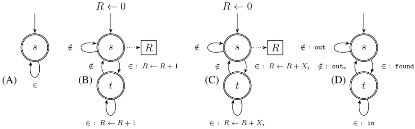
3.1 (A) Automaton recognising the signatures of integer sequences whose elements are all in {−1, 0, 5}. (B) Register automaton recognising any signature and returning the number of elements in {−1, 0, 5} in an integer sequence. (C) Register automaton recognising any signature and returning the sum of elements in {−1, 0, 5} in an integer sequence. (D) Trans-ducer with the input alphabet {2, /2} and the output alphabet {found, out, in, outa} . . . 33
3.2 (A) Automaton recognising sequences of 0 and 1, where 0 are only located at odd positions; (B) automaton recognising sequences of 0 and 1, where 1 are only located at even positions; (C) intersection of (A) and (B); (D) complement of (A). . . 34
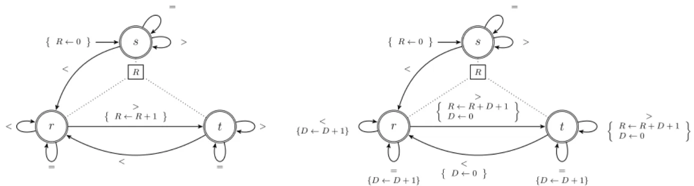
3.3 (A) and (B) register automata over alphabet {<, =, >}; (C) intersection of (A) and (B) . . 35
5.1 Time series h0, 1, 2, 2, 0, 0, 4, 1i with its two peaks of respective widths 3 and 1 . . . 46
5.2 Seed transducer for thePEAKregular expression. This figure is adapted from [10]. . . 48
5.3 Register automata forNB_PEAKand SUM_WIDTH_PEAK. These figures are adapted from [10]. . . 49
5.4 Simplified register automata for NB_PEAK (left) and SUM_WIDTH_PEAK (right). These figures are adapted from [10]. . . 50
5.5 (A) Features: the function used for computing the value of a feature. (B) Decoration table used for synthesising the register automaton for a time-series constraint . . . 51
5.6 (A) The prefix h0, 1, 2i of the time series h0, 1, 2, 2, 0, 0, 4, 1i without any peaks. (B) The suffix h2, 2, 0, 0, 4, 1i of the time series h0, 1, 2, 2, 0, 0, 4, 1i with one peak . . . 52
6.1 Regular-expression characteristics introduced in Chapters 7 and 8. . . 61
6.2 Seed transducer for σ = DECREASING_TERRACEwhen bσ is 1 (A) and 2 (B) . . . 64
7.1 Illustration of the introduced regular-expression characteristics . . . 74
7.2 Lemma 7.2.2 Case (1.1): Illustration of the word z1w1w2w1w2 belonging to the language of ‘v | z1(w1w2)⇤(w1| ")’ . . . 82
8.1 Time series illustrating the introduced regular-expression characteristics . . . 99
8.2 Time series illustrating the intuition of theAMONGimplied constraints . . . 103
9.1 (A) Register automaton forNB_PEAK. (B) Register automaton forNB_VALLEY. (C) Inter-section of (A) and (B). . . 111
10 LIST OF FIGURES
9.2 Invariant digraph forNB_PEAKandNB_VALLEYwrt e + e0· n + e1· P + e2· V . . . 112
9.3 (A) The invariant digraph of the register automata for two time-series constraints. (B) The set of feasible values of the result variables of two constraints . . . 115
9.4 Intersection of the register automata for two time-series constraints, for which our method does not generate sharp linear invariants . . . 117
9.5 Delayed intersection obtained from the intersection in Figure 9.4 . . . 118
9.6 Invariant digraph obtained from the delayed intersection in Figure 9.5 . . . 120
9.7 (A) General linear invariants, (B) linear invariants with non-default value conditions for a pair of time-series constraints. (C) Automaton with guard invariants . . . 121
9.8 Illustration of infeasible combinations of the result values of time-series constraints not eliminated by the generated linear invariants . . . 123
10.1 Feasible and infeasible combinations of the result values of two time-series constraints im-posed on the same sequence whose length is in {9, 10, 11, 12} . . . 127
10.2 Seven groups of infeasible combinations of the result values of two time-series constraints 131 10.3 (A) Automaton for a gap atomic relation. (B) Automaton for a modulo atomic relation . . 133
10.4 Illustration of infeasible combinations of the result values not eliminated byt the generated non-linear invariants . . . 133
11.1 (A) Register automaton forSUM_WIDTH_DECREASING_SEQUENCE(X, R). (B) Automa-ton for the R = 3 constant atomic relation. (C) All signatures of length 3 accepted by the automaton in Part (B) . . . 136
11.2 (A) Register automaton for NB_DECREASING_SEQUENCE(X, R). (B) Automaton for the R mod 2 = 1 atomic relation. (C) All signatures of length 2 accepted by the automaton in Part (B) . . . 138
11.3 (A) Automaton achieving the maximum number of peaks in a time series of length n. (B) All corresponding accepted words for n − 1 2 {4, 5}. (C) The signatures of time series with gap 1 and 2, respectively, and with loss 3 and 5, respectively . . . 140
11.4 Illustration of gap and loss for six time series . . . 143
11.5 Seed transducer (A) and separated seed transducer (B) for thePEAKregular expression. . . 149
11.6 Loss automaton forNB_PEAK. The initial value of the registers C, D, and R is zero. . . . 151
12.1 Well-formed output language . . . 161
12.2 New seed transducers for 5 regular expressions . . . 163
12.3 Trace for theMAX_WIDTH_GROUPconstraint . . . 165
13.1 Comparing backtrack count and runtime for Automaton and its variants . . . 172
13.2 Scalability results comparing time for Automaton and Combined on problems of increasing length. . . 173
13.3 Comparing parts of the search tree for MAX_SURF_INCREASING_TERRACE, finding the first solution or proving infeasibility . . . 174
14.1 Comparing backtrack count and runtime of the g_f_σ time-series constraint for previous best results and new method for finding the first solution or proving infeasibility . . . 176
15.1 Comparing constraint variants, undecided instances percentage for size 18 as a function of time . . . 178
15.2 Percentage of problems solved for 3 overlapping segments of lengths 22, 24, and 25. . . . 179
17.1 Synthesised combinatorial objects, grouped by the case they are synthesised for, i.e. char-acterising a single constraint or a conjunction of constraints . . . 184 17.2 Les objets combinatoires synthétisés et les facettes à partir desquelles ils étaient synthétisés 189
List of Tables
5.1 Features and aggregators . . . 44
5.2 Regular-expression names σ, corresponding regular expressions, and values of the parame-ters aσand bσ. This table is adapted from [14]. . . 45
5.3 Glue matrix for theNB_PEAKconstraint . . . 52
5.4 Comparison of time-series constraints and QREs . . . 53
7.1 Regular-expression names and corresponding size, height, range, set of inducing words, overlap and smallest variation of maxima . . . 75
7.2 A synthesis of all the bounds presented in Sections 7.2, 7.3, and in [8]. . . 93
7.3 Classification of regular expressions: regular expression names σ, their properties and con-ditions on domain [`, u] when they hold. . . 94
8.1 Regular expressions and corresponding maximum value occurrence number and big width. 102 8.2 Regular expressions and corresponding interval of interest and the lower bound on the pa-rameter of theAMONGimplied constraints for theMAX_SURF_σ family . . . 105
8.3 Regular expressions and corresponding interval of interest and the lower bound on the pa-rameter of theAMONGimplied constraints for theSUM_SURF_σ family . . . 106
11.1 Decoration table for the loss automaton forNB_σ time-series constraints . . . 150
12.1 Features and aggregators of the extended transducer-based model . . . 157
12.2 Illustration of s-occurrences of a concrete pattern in a signature, and of their corresponding found indices, e-occurrences and i-occurrences . . . 158
12.3 Operational views of features and aggregators in the extended transducer-based model . . 159
12.4 Examples of functions over integer sequences . . . 159
16.1 Comparing the state-of-the-art baseline and the baseline with the generated invariants . . . 181
C.1 Table for the size regular-expression characteristic . . . 211
C.2 Table for the height regular-expression characteristic . . . 212
C.3 Table for the range regular-expression characteristic . . . 213
C.4 Table for the set of inducing words regular-expression characteristic . . . 214
C.5 Table for the overlap regular-expression characteristic . . . 215
C.6 Table for the smallest variation of maxima regular-expression characteristic . . . 216
C.7 Table for the interval of interest regular-expression characteristic . . . 218
C.8 Table for the maximum value occurrence number regular-expression characteristic . . . 220
C.9 Table for the big width regular-expression characteristic . . . 222
Chapter 1
Introduction
1.1
Tradeoff Between the Expressiveness of a Modelling Language
and the Efficiency of Solving for Combinatorial Problems
Many real-life problems, e.g. staff scheduling in a call centre or production planning of a power plant, can be described as mathematical models. In such a context, we have two main aspects: 1) the modelling language aspect, i.e. our language should be rich enough to concisely express a large variety of problems; 2) the solving aspect, i.e. we should be able to find a solution to our model efficiently. Currently, we face one of the two following situations:
1. We have a powerful language allowing us to model easily and that can be further extended. However, the solving aspect is highly inefficient.
2. Our language is restricted and extending the language may require adding ad hoc elements specific to a considered problem, but not useful for any other problem.
Within the context of problems using integer sequences, the goal of this thesis is to obtain a tradeoff between the expressiveness of the modelling language and the efficiency of the solving aspect for com-binatorial problems. We work towards a language that is powerful enough to describe a large variety of problems, and efficient enough from the solving point of view. Our approach is based on the following observation: any model for a combinatorial problem has two main components, namely 1) variables that represent quantities, e.g. produced amount of electricity for a given power plant, and take their values in given sets, called domains, and 2) constraints, which impose relations between these variables and repre-sents business processes, technical restrictions, etc. Such models often use discrete objects such as
— permutations [117];
— trees [42], i.e. acyclic connected graphs;
— time series [47], i.e. integer sequences representing measurements taken over time.
Such discrete objects can be described by their characteristics, e.g. the number of cycles in a permutation [82], the diameter of a tree [104], and the number of peaks in a time series [22]. Characteristics are often used to represent the constraints of the problem. In the solving context, we typically need to find a discrete object simultaneously satisfying restrictions on its several characteristics, e.g. a time series with 3 peaks and 2 valleys. Restricting several characteristics may be more challenging than restricting a single characteristic since during the solving phase constraints have to communicate efficiently, which is not always the case.
1.2
Mathematical Programming and Constraint Programming
for Modelling and Solving Combinatorial Problems
Mathematical Programming(MP) [126] and Constraint Programming (CP) [118] are two complemen-tary approaches for modelling and solving combinatorial problems using discrete objects with a number of
14 CHAPTER 1. INTRODUCTION
successful applications in the domains of scheduling, packing, and routing [134, 135, 48, 51, 110, 95, 65]. The main difference between CP and MP are the types of constraints used for modelling. In the context of MP, constraints are usually linear or convex [16, 33, 115], and, for example, for problems with only linear constraints, solvers typically use the simplex method [58]. CP models use global constraints. The Global Constraint Catalogue [21] defines a global constraint as “an expressive and concise condition involving a non-fixed number of variables”. For example, the ALLDIFFERENT(hX1, X2, . . . , Xni) [130] global
con-straint restricts a sequence of integer variables hX1, X2, . . . , Xni to take distinct values. Therefore, the
sequence h1, 8, 7, −1, 3i satisfies anALLDIFFERENTconstraint, but h1, 8, 1, −1, 3i does not since X1 is the
same as X3. In CP, a global constraint usually comes with a filtering technique, which is an algorithm or
any kind of inference that allows one to reduce the domains of the variables by removing values that cannot be part of any solution to this constraint.
Despite different constraint types, and thus different solving techniques, CP and MP have some common drawbacks that motivate the work of this thesis:
◦ In both MP and CP, modelling can be challenging both from the point of view of problem description and from an inference point of view. In MP, this is due to the fact that constraints must be linear or convex. In CP, this is due to the fact that a required global constraint may not exist and needs to be introduced. Hence there is a common need to define constraints in a compositional way that can be then systematically reformulated as linear programs or for which one can obtain a filtering technique in a systematic way.
◦ When domains of variables are discrete, both MP and CP models may become hard to solve [106, 131]. Hence in order to solve a problem efficiently one tries to draw full benefit from the structure of the considered problem. In MP, this is done in the preprocessing step, where a solver verifies whether a considered problem has a well-known structure, e.g. network flow [63], and then applies a specific preprocessing technique for this subproblem and/or generates cuts [75, 96]. In CP, this is done by designing dedicated filtering techniques for global constraints of the problem. Hence there is a need to synthesise combinatorial objects characterising the structure of a considered combinatorial problem, e.g. bounds, linear cuts, implied constraints, which are redundant constraints that do not change the set of solutions of the problem, but their purpose is to remove infeasible values from the domains of the variables.
◦ The need to exploit the problem structure leads to a large number of ad hoc methods, e.g. specific bounds, algorithms, decompositions, filtering techniques, heuristics. These are methods that are efficient for solving the problem they were designed for, but either cannot be reused at all for any other problem or require a significant effort for adjusting them. Hence there is a need to develop systematic methodsfor synthesising combinatorial objects for constraints occurring in a considered problem.
1.3
Context of Our Work: Time-Series Constraints
This thesis studies a family of global constraints, called time-series constraints, defined in a compo-sitional way by means of functions [22, 10]. A time-series constraint γ(X, R) restricts R, called the result value of γ, to be the result of some computations over the sequence of integer variables X = hX1, X2, . . . , Xni, called a time series, which represents measurements taken over time [22]. For
ex-ample, R could be the number of consecutive pairs of variables hXi, Xi+1i of X such that Xi < Xi+1
with i in [1, n − 1]. The three main ingredients describing a time-series constraint are a pattern, a fea-ture, and an aggregator. A pattern is some regular form of subsequences, which is from a formal point of view characterised by a regular expression over the alphabet of three letters {‘<’, ‘=’, ‘>’}. For ex-ample, theDECREASING_SEQUENCE pattern, which corresponds to any maximal monotonously
1.4. THE TWO TOPICS OF THIS THESIS 15
‘(> (> | =)⇤)⇤ >’ regular expression, which relates the variables of the subsequence hX
i, Xi+1, . . . , Xji as
follows:
◦ Xi > Xi+1, i.e. this subsequence starts with a strict decrease;
◦ Xj−1 > Xj, i.e. this subsequence also ends with a strict decrease;
◦ for any k in [i + 1, j − 2], we have that Xk ≥ Xk+1, i.e. in the middle this subsequence can either
decrease or stay at the same level.
For example, in the h1, 2, 0, 0, −1, 3, 4, 2, 2i time series there are two decreasing sequences, namely h2, 0, 0, −1i and h4, 2i. Note that although h2, 0i satisfies the conditions on the relations between its values, it is included in h2, 0, 0, −1i, and thus is not maximal.
A feature and an aggregator are functions over integer sequences, e.g. the maximum of a sequence of integers, or the sum of elements in an integer sequence.
Time series are very common in many real-life applications. We now give a few examples of possible usage of time-series constraints:
◦ Analysis of the output of electric power stations over multiple days in the context of solving the unit commitment problem [28]. From known production curves of power plants one can extract a model using time-series constraints, and then generate similar production curves satisfying additional re-strictions for a considered power plant.
◦ Modelling a problem of staff scheduling in a call centre [11]. The overall problem is to cover the given manpower demand over time, while minimising overall resource cost, and at the same time satisfying restrictions related to business processes, employment rules, and union contracts, which can be expressed as time-series constraints.
◦ Data mining in the context of power management for large-scale distributed systems [26].
◦ Trace analysis for Internet Service Provider to test the bandwidth of the user’s Internet connex-ion [66].
◦ Anomaly detection and error correction in the temperature in a building [113].
◦ Real-time decision-making, for example, where one needs to analyse data streams in order to adjust the toll rate depending on the traffic [5].
1.4
The Two Topics of this Thesis
The first topic of this thesis is developing systematic methods for synthesising compositional combi-natorial objectssuch as bounds, linear invariants, automata for time-series constraints. The main idea is to exploit the compositional nature of time-series constraints at the combinatorial level, i.e. the level related to the solution space associated with a constraint or a conjunction of constraints. Compositionality here means that we can combine such objects during the solving phase and also we can use them with different technologies and/or in different contexts, e.g. CP, MP, data mining.
A formula typically captures some combinatorial relation between different quantities. The idea put forward in this thesis is based on the bet that, provided that it is possible to synthesise them, the set of formulae and redundant constraints potentially has more impact than a set of dedicated algorithms. Indeed, from a compositional point of view, formulae can be used conjointly and applied in the context of several resolution techniques such as CP or MP, which is much more difficult in the context of algorithms. As we will see in the benchmarks of Part III, yet another advantage of combinatorial objects is synergy between them, i.e. we can compose them. Different combinatorial objects combined together provide us with better performance than when used separately. A vibrant example of such synergy is the interaction of bounds on the result value of a time-series constraint γ and glue constraints [8, 23]. For a sequence of variables X = hX1, X2, . . . , Xni, a prefix P = hX1, X2, . . . , Xii and a reversed suffix S = hXn, Xn−1, . . . , Xii of
X, a glue constraint links the result values of three time-series constraints γ imposed on X, on P , and on S. Synthesised combinatorial objects can be used for different purposes including, but not limited to:
16 CHAPTER 1. INTRODUCTION Time-Series Constraint (declarative view) Regular Expression Time-Series Constraint (operational view) Transducer # Register Automaton
◦ Bounds on the result value ◦ AMONGimplied constraints
◦ Linear invariants ◦ Non-linear invariants ◦ Conditional automata
Figure 1.1 – Synthesised combinatorial objects and the facets from which they were synthesised, i.e. declarative with regular expressions or operational with transducers and/or register automata. An arrow from source to destination indicates that destination can be synthesised from source.
values of variables as possible since the smaller are the domains, the easier it is to find a solution. Synthesised combinatorial objects can be used for making the pruning of time-series constraints stronger.
◦ While time-series constraints can be reformulated as linear models [11] and integrated into existing linear models, the obtained linear reformulation is not tight, i.e. a linear programming solver such as CPLEX or Gurobi typically spends a lot of time to solve it. Our combinatorial objects can be used to fasten the solving aspect in the context of linear programming.
◦ Time-series constraints can be used in the context of data mining. For example, bounds on the result value of a time-series constraints are used for clustering time series representing the workload of a data centre [94]; bounds allow us to compare the maximum ranges of variation of the result values of different time-series constraints.
From the operational point of view, every time-series constraint γ has a representation by a register automaton, which is synthesised from the seed transducer for a regular expression associated with γ [22]. It was shown in [68] how to automatically generate a seed transducer from a regular expression. All com-binatorial objects we obtain in this thesis will be either synthesised from the declarative view of time-series constraints, i.e. using regular expressions, or from their operational representation, i.e. using register au-tomata and seed transducers. Figure 1.1 gives the classification of the combinatorial objects depending on the representation of time-series constraints, from which they were synthesised, i.e. declarative or opera-tional. The combinatorial objects presented in Figure 1.1 will be further detailed in Section 1.6.
While using transducers and automata has a long-standing tradition in the context of synthesising reli-able software components [133, 128], it is rarely used to synthesise combinatorial objects such as bounds, cuts or glue constraints. However one can point out the following correspondence between computer-aided verification [55] and constraint programming: first, both use sometimes high-level declarative specifica-tions from which transducers and or automata are synthesised. Second, there is a correspondence between invariants that are typically extracted from these transducers and automata for proving some property of a program or a system, and the necessary conditions one would like to synthesise in the context of CP or MP to get stronger inferences: both are formulae that must always be true.
The second topic of this thesis is the extension of the approach used for describing time-series con-straintsto capture a larger number of sequence constraints such as [25, 105, 108]. The initial work [22] uses finite transducers to synthesise filtering techniques for time-series constraints. However, the same
1.5. DIFFERENCES WITH EXISTING APPROACHES 17
transducer-based model can be extended for synthesising filtering techniques for other global constraints such asAMONG[25],SIMILARITY[105], andSTRETCH[108].
1.5
Differences with Existing Approaches
Before giving an overview of our contributions, we state four reasons that distinguish our work from other approaches:
◦ First, in the literature there are approaches that either focus on the combinatorial aspect of specific constraints such as ALLDIFFERENT, REGULAR, NVALUE [116, 19, 39, 41] or propose generic
ap-proaches for describing constraints and synthesising filtering techniques [129, 100, 73]. Some of the approaches do not automatically handle the combinatorial aspect of a constraint: they rely on the user to describe a filtering technique by a set of formulae [129, 100]. In the others, the set of solutions to the constraint is represented by a multi-valued decision diagram (MDD) [35, 107] that can be exponential in size. Some works are devoted to synthesis of an approximation of MDDs of a smaller size [76]. However, MDDs do not focus on the relations between different characteristics of discrete objects. In our work, we go a step further and explore the topic of automatically synthe-sisingpropagators in the form of combinatorial objects for the large class of time-series constraints [22] involving more than 200 constraints.
◦ Second, the obtained combinatorial objects can be used, not only as propagators in the context of constraint programming, but also in the context of linear programming, data mining, local search. This implies that such objects represent essential information about the combinatorial aspect of a time-series constraint, and thus are independent of the context in which time-series constraints are used.
◦ Third, the obtained objects are parameterised by the description of a considered time-series con-straint, the length of a time series, and the domains of the time-series variables, and are synthesised once and for all. This allows us to create a database of combinatorial objects for time-series con-straints [10] and consult it in completely different contexts every time when required. There is no need to rerun our methods for synthesising these combinatorial objects for each problem instance. Note that, in order to obtain such combinatorial objects, we have to automatically prove that they are valid for any sequence length.
◦ Fourth, working towards uniform ways of representing families of global constraints and of han-dling their combinatorial aspect is not common within the CP community, but is still important since otherwise we would end up with a set of dedicated constraints for each problem that do not communicate.
1.6
A Guided Tour Through the Main Contributions of this Thesis
The main contributions presented in this thesis are the following:
◦ [Parameterised upper and lower bounds on the result value of every time-series constraint] A bound formula for a considered time-series constraint is parameterised by the time-series length n, and the domains of the time-series variables. Each bound formula is obtained from some generic formula, which is parameterised by a considered time-series constraint. Hence we only need to prove very few generic formulae, i.e. less than 10, rather than one formula per time-series constraint, i.e. more than 200. While the bound is always valid, its sharpness is only guaranteed when the domains of all series variables correspond to the same integer interval. For almost all time-series constraints, both upper and lower bounds are evaluated in constant time, except 12 time-time-series constraints, for which it takes O(n) to evaluate the bound [8].
18 CHAPTER 1. INTRODUCTION 0 2 4 10 À Ã Õ Œ
Figure 1.2 – The time series h3, 2, 4, 2, 4, 1, 3, 2, 3, 0i with the maximum (five) number of decreasing se-quences among any time series of length 10. The horizontal axis is for time-series elements, and the vertical axis is for the values. The dashed lines separate different decreasing sequences.
This work was published in the Constraints journal [14] and in the proceedings of the CP’16 con-ference [8], and the bounds for all time-series constraints were integrated into the Volume II of the Global Constraint Catalogue [10].
Example 1.6.1 (sharp bounds). Consider a sequence of integers X = hX1, X2, . . . , Xni. A
de-creasing sequencein X is a maximal inclusion-wise monotonously decreasing subsequence of X. For example, the sequence h1, 2, 1, 0, 0, −1, −2, 2, 4, 2, 2i has two decreasing sequences, namely h2, 1, 0, 0, −1, −2i and h4, 2i. Since each decreasing sequence contains at least two elements and any two decreasing sequences never overlap, the maximum number of decreasing sequences in X is⌅n
2⇧. Hence for the NB_DECREASING_SEQUENCE(hX1, X2, . . . , Xni , R) time-series constraint,
where R is constrained to be the number of decreasing sequences in hX1, X2, . . . , Xni, a sharp upper
bound on R is⌅n
2⇧. For example, Figure 1.2 gives a time series of length n = 10 with 5 decreasing
sequences, which is the maximum possible number of decreasing sequences in any time series of length 10. The formula⌅n
2⇧ is a special case of a generic formula of Theorem 7.2.2, on 84, that gives
the number of maximal inclusion-wise occurrences of a pattern in a sequence of integer numbers. In this example, the pattern isDECREASING_SEQUENCE. 4
◦ [ParameterisedAMONGimplied constraintsfor three families of time-series constraints]
An AMONG global constraint [25] restricts the number of variables of a sequence of variables to
take their values in a particular finite set of integer values. Here, the word implied means that these constraints are redundant, i.e. they do not change the set of solutions of the problem, but their purpose is to remove infeasible values from the domains of the variables. Similar to bounds, there is one per family genericAMONG implied constraint that is parameterised by the pattern of a
considered time-series constraint. Hence we only need to prove three AMONGimplied constraints
in order to further use them for 66 time-series constraints.
This work was published in the proceedings of the CP’17 conference [12], and theAMONGimplied
constraints for 66 time-series constraints were integrated in the Volume II of the Global Constraint Catalogue [10].
Example 1.6.2(AMONGimplied constraints, example adapted from [12]). Consider theMAX_SURF_ DECREASING_SEQUENCE(X, R) time-series constraint, where X is a sequence of integer variables of length n, and R is constrained to be the maximum of the sums of the elements of the decreasing sequences of X. For example, the sequence h1, 2, 1, 0, 0, −1, −2, 2, 4, 2, 2i has two decreasing se-quences, namely h2, 1, 0, 0, −1, −2i and h4, 2i, with a sum of elements 0 and 6, respectively. The maximum of these two values is 6, and thus R is fixed to 6.
Now assume that the value of R is known and is equal to, for example 18, but X is unknown, and our goal is to find a sequence X of 7 integers, which are all in [1, 4], such that X yields 18 as the value of R. By enumerating all integer sequences satisfying these restrictions, we observe that any such integer sequence contains a single decreasing sequence with at least 4 its elements being 3 or 4. This allows us to the state theAMONG(N, hX1, X2, . . . , X7i , h3, 4i) constraint with N ≥ 4, which
1.6. A GUIDED TOUR THROUGH THE MAIN CONTRIBUTIONS OF THIS THESIS 19
means that the number N of occurrences of the values 3 and 4 in the sequence hX1, X2, . . . , X7i is
at least 4.
The parameters of theAMONGimplied constraint, i.e. h3, 4i in this example, and a lower bound on
N are obtained from a generic formula, parameterised by the pattern associated with a time-series
constraint. 4
◦ [Parameterised linear implied inequalities linking the result values of a conjunction of time-series constraints imposed on the same time series of length n]
We explore the relations between the result values of several time-series constraints imposed on the same time series. We call these inequalities linear invariants.
This work was published in the proceedings of the CP’17 conference [13], and the obtained linear inequalities were integrated in the database of invariants of the Volume II of the Global Constraint Catalogue [10].
Example 1.6.3(Linear invariants). Consider the conjunction ofNB_DECREASING_SEQUENCE(X, R1) and NB_INCREASING_SEQUENCE(X, R2) imposed on the same sequence of variables X of
length n, where R1(respectively R2) is constrained to be the number of decreasing (respectively
in-creasing) sequences in X. An increasing sequence in X is a maximal inclusion-wise monotonously increasing subsequence of X. Since between any two consecutive increasing sequences there is ex-actly one decreasing sequence and vice versa, the linear inequalities R1 R2+ 1 and R2 R1+ 1
hold for any sequence X of integers. In addition, the total number of decreasing and increasing se-quences in an integer sequence of length n cannot exceed n. Hence the linear inequality R1+R2 n
holds for any sequence X of any length n.
We extract such linear invariants using register automata associated with the corresponding
time-series constraints. 4
◦ [Parameterised non-linear invariants linking the result values of a conjunction of time-series con-straints imposed on the same time series of length n]
Such invariants characterise sets of infeasible combinations of the result values of the time-series constraints in a conjunction that cannot be described as a linear combination of the result values of the conjunction of time-series constraints and n. In other words, these are sets of infeasible combinations that are located within the convex hull of feasible combinations.
The obtained non-linear invariants were integrated in the database of invariants of the Volume II of the Global Constraint Catalogue [10].
Example 1.6.4(Non-linear invariants). Consider the conjunction ofSUM_WIDTH_DECREASING_
_SEQUENCE(X, R1) andSUM_WIDTH_INCREASING_SEQUENCE(X, R2) imposed on the same
se-quence of variables X of length n, where R1 (respectively R2) is constrained to be the sum of the
number of elements of all decreasing (respectively increasing) sequences in X. For example, the in-teger sequence h1, 2, 1, 0, 0, −1, −2, 2, 4, 2, 2i has two decreasing sequences, namely h2, 1, 0, 0, −1, −2i and h4, 2i, with 6 and 2 elements, respectively, i.e. of width 6 and 2; and two increasing se-quences, namely h1, 2i and h−2, 2, 4i, with 2 and 3 elements, respectively, i.e. of width 2 and 3. Hence R1 (respectively R2) is constrained to be the sum of 6 and 2 (respectively 2 and 3), which is
8 (respectively 5).
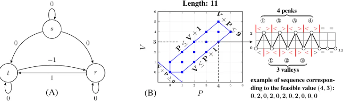
By generating all feasible combinations of R1 and R2 for sequences of length 9, 10, 11 and 12, we
observe that there are quite a few infeasible pairs of R1and R2that are located within the convex hull
of feasible pairs. The generated combinations are reported in Figure 1.3. Our goal is to synthesise and prove such generic non-linear invariants linking R1, R2 and parameterised by a function of n
stating that the points depicted by red circles in Figure 1.3 are infeasible. For example, the five invariants that we obtain for the considered pair of constraints are
20 CHAPTER 1. INTRODUCTION 0 2 4 6 8 10 0 2 4 6 8 10 sum_width_decreasing_sequence sum_width_increasing_sequence Sequence length: 9 0 2 4 6 8 10 0 2 4 6 8 10 sum_width_decreasing_sequence sum_width_increasing_sequence Sequence length: 10 0 2 4 6 8 10 12 0 2 4 6 8 10 12 sum_width_decreasing_sequence sum_width_increasing_sequence Sequence length: 11 0 2 4 6 8 10 12 0 5 10 sum_width_decreasing_sequence sum_width_increasing_sequence Sequence length: 12 9 0 2 <><><><> ¨ ≠ Æ Ø
4 decreasing sequences of width2
z }| {
<><><><>
¨ ≠ Æ Ø
| {z }
4 increasing sequences of width2 example of sequence corresponding
to the feasible pair(8, 8): h0, 2, 0, 2, 0, 2, 0, 2, 0i
Figure 1.3 – Feasible (blue squares) and infeasible (red circles) combinations of the results val-ues R1 and R2 of the constraints SUM_WIDTH_DECREASING_SEQUENCE(X, R1) and SUM_WIDTH
_INCREASING_SEQUENCE(X, R2) imposed on the same sequence X whose length is in {9, 10, 11, 12}.
We represent only infeasible combinations that are located within the convex hull of all feasible combina-tions.
1.6. A GUIDED TOUR THROUGH THE MAIN CONTRIBUTIONS OF THIS THESIS 21
• R2 6= 1,
• R1 6= n _ R2 mod 2 = 0,
• R2 6= n _ R1 mod 2 = 0,
• n mod 2 = 1 _ R1 6= n − 1 _ R2 6= n − 1.
Note that some of these invariants are parameterised by functions of n, namely n − 1 and n mod 2. Note also that these invariants hold for any integer sequence X of any length n. 4
◦ [Constant-size automata representing the set of all integer sequences satisfying some condition, e.g. all integer sequences with the maximum possible number of decreasing sequences for a given sequence length]
On the one hand, finite automata are used since the beginning of computer science to model many aspects of computation [81]. On the other hand, bounds are ubiquitous in a number of optimisation problems [88, 18], where they allow one to speed up the search process. While bounds are typically expressed as parameterised formulae [30, 14], the question of a compact and explicit representation of the set of all solutions reaching a particular bound went unnoticed. Such automata are a crucial part of our method for synthesising and proving non-linear implied constraints, mentioned in the previous item.
The obtained automata were integrated in the Volume II of the Global Constraint Catalogue [10]. Example 1.6.5(Constant-size automata). Consider theNB_DECREASING_SEQUENCE(X, R) time-series constraint introduced in Example 1.6.1, where X is a sequence of variables of length n. Recall that the maximum number of decreasing sequences in a sequence of length n is⌅n
2⇧. With any
inte-ger sequence X we can associate a sequence of binary relations in {<, =, >} between every pair of its consecutive variables. We name such sequence the signature of X. For example, the signature of the sequence h1, 2, 0, 2, 3, −1i is h<, >, <, <, >i. The constant-size automaton M in Part (A) of Figure 1.4 accepts the signatures of all and only all integer sequences with the maximum number of decreasing sequences, i.e. sequences for which the constraintNB_DECREASING_SEQUENCE(X,⌅n
2
⇧ ) holds. The state s is the initial state of M, and the states s, t, and t0are accepting states. A transition
labelled with a binary operator ◦ in {<, =, >} is triggered iff for the current consecutive pairs of values Xi and Xi+1, the corresponding binary relation ◦ holds. Part (B) gives all the signatures of
lengths 3 and 4 accepted by this automaton. 4
◦ [An extended transducer-based computational model describing functions over integer sequences arising in the context of constraint programming]
The extended model covers time-series constraints, but also most sequence constraints in the Volume I of the Global Constraint Catalogue [21].
t s t0 s0 > < > < = < > = (A) > < > = > < > < > < > > = < > > > < > (B) > < = > > < > > > < > = > < > < > < < >
Figure 1.4 – (A) Automaton accepting the signatures of all, and only all, integer sequences with the max-imum number of decreasing sequences. (B) All signatures of lengths 3 and 4 accepted by the automaton in (A).
22 CHAPTER 1. INTRODUCTION Summary of our Contributions:
◦ Systematic methods for synthesising objects, namely automata and formulae, e.g. bounds, linear and non-linear invariants,AMONGimplied constraints that
1. capture the combinatorial flavour of a considered time-series constraint or a conjunction of time-series constraints,
2. are parameterised by a considered instance, i.e. the domains of the variables and the sequence length, and a considered time-series constraint,
3. can be used in different contexts.
◦ Extension of a transducer-based model used for describing time-series constraints, which provides us with a uniform way of representing sequence constraints.
1.7
The Reading Grid of this Thesis
We present the plan of this thesis as well as a reading grid, which consists of three main parts:
1. Background, containing all necessary information for understanding this thesis. This includes topics such as regular expressions in Chapter 2, register automata and transducers in Chapter 3, constraint programming in Chapter 4, and time-series constraints in Chapter 5. When presenting time-series constraints we will consider both their declarative view, given in Section 5.1, and their operational view, given in Section 5.2.
2. Theoretical Contributions, which gives first a detailed overview of our contributions for synthesis-ing combinatorial objects for time-series constraints and extendsynthesis-ing a transducer-based computational model, and then presents the following contributions:
◦ Parameterised bounds, presented in Chapter 7. Considered context: constraint in isolation.
Required background: Chapter 2 (regular expressions), Chapter 4 (constraint programming),
Section 5.1 (declarative view of time-series constraints). ◦ ParameterisedAMONGimplied constraints, presented in Chapter 8.
Considered context: constraint in isolation.
Required background: Chapter 2 (regular expressions), Chapter 4 (constraint programming),
Section 5.1 (declarative view of time-series constraints). ◦ Parameterised linear invariants, presented in Chapter 9.
Considered context: conjunction of constraints.
Required background: Chapter 3 (automata and register automata), Chapter 4 (constraint programming),
Section 5.2 (operational view of time-series constraints). ◦ Parameterised non-linear invariants, presented in Chapter 10.
Considered context: conjunction of constraints.
Required background: Chapter 3 (automata and register automata), Chapter 4 (constraint programming),
Section 5.2 (operational view of time-series constraints). ◦ Conditional constant-size automata, presented in Chapter 11.
Considered context: conjunction of constraints.
Required background: Chapter 3 (automata and register automata), Chapter 4 (constraint programming),
1.7. THE READING GRID OF THIS THESIS 23
◦ Extended transducer-based model, presented in Chapter 12.
3. Practical Evaluation, contains the practical evaluation of the impact of the synthesised combinatorial objects.
Part I
Background
27 In this part, we give the necessary background for understanding this thesis. We now introduce the chapters of this part and explain their importance in the context of this work:
◦ As mentioned in Chapter 1, a pattern is one of the three main components of a time-series constraint. From a formal point of view, a pattern is a regular expression [57], which describes a regular lan-guage.
Chapter 2 gives background on regular expressions and regular languages.
◦ From an operational point of view, regular languages can be represented by finite automata [80]. A finite automaton consists of a finite number of states and transitions between states, labelled with input symbols. It consumes an input sequence and either accepts this sequence or fails. With every automaton we can associate a regular expression whose regular language is accepted by this automaton and vice versa. Finite transducers [119] are automata that not only consume an input sequence but also produce an output sequence. Register automata [20] are automata augmented with a constant number of registers that are used to perform computations over an input sequence, e.g. count the number of decreasing sequences in an integer sequence.
Chapter 3 gives background on automata, transducers, and register automata.
◦ An important notion of CP is a constraint satisfaction problem (CSP) [118], which consists of variables with finite domains and constraints. Typically in the CP context we are searching for a solution to a CSP using filtering techniques for constraints of the problem. Automata and register automata can be used to filter some global constraints. For a sequence of variables of a fixed length, an automaton or a register automaton can be decomposed as a conjunction of logical constraints [29]. The number of variables and constraints in such a conjunction depends linearly on the length of an input sequence.
Chapter 4 gives a formal definition of constraint satisfaction problem, mentions the most common techniques for solving a CSP, and also gives examples of global constraints, for which automata and register automata are used for both describing these constraints and also for filtering them.
◦ Time-series constraints [22] are a central part of the work of this thesis. Due to their compositional nature, a single definition is used for obtaining more than 200 constraints for 22 patterns. Register automata can be used to filter time-series constraints. Because of the large number of time-series constraints we have to synthesise register automata in a systematic way as follows:
1. Generate a finite transducer whose output sequence identifies all maximal occurrences of the pattern [68].
2. Replace in the transducer every output symbol with a set of register updates corresponding to the feature and the aggregator [22].
Chapter 2
Background on Regular Expressions
In this chapter, which is adapted from [14], we give the background on regular expressions, which are one of the key ingredients of time-series constraints.
An alphabet A is a finite set of symbols, and a symbol of A is called a letter. A word on A is a finite sequence of symbols belonging to A. The empty word is denoted by ". The length of a word w is the number of letters in w and is denoted by |w|. For i 2 [1, |w|], w[i] denotes the ith letter of a word w. The
concatenation of two words is denoted by putting them side by side, with an implicit infix operator between them. A word w is a factor of a word x if there exist two words v and z such that x = vwz; when v = ", w is a prefix of x, when z = ", w is a suffix of x. If both w is not empty and different from x, then it is a proper factor of x. Given a word w and a positive integer k > 0, wkdenotes the concatenation of k occurrences of
w. Given an integer k and a language L, Lk is defined by L0 = {"}, L1 = L and Lk = L · Lk−1 where ‘·’
is the concatenation operator. Then the Kleene closure of L is defined by [n≥0Lnand denoted by L⇤.
Definition 2.0.1(Regular expression [57]). A regular expression r on an alphabet A and the language Lrit
describes, the regular language, are recursively defined as follows:
(1) 0 and 1 are regular expressions that respectively describe ; (the empty set) and {"}. (2) For every letter ` of A, ` is a regular expression that describes the singleton {`}.
(3) If r1 and r2 are regular expressions, respectively describing the regular languages Lr1 and Lr2, then
r1+ r2, r1· r2 and r⇤1are regular expressions that respectively describe the regular languages Lr1[ Lr2,
Lr1 · Lr2, and L
⇤ r1.
Example 2.0.1 (Regular expressions over the alphabet associated with time-series constraints). Consider the alphabet Σ = {‘<’, ‘=’, ‘>’}.
• DECREASING = ‘>’ is a regular expression on Σ. The word v = ‘>’ is a word of length 1 on Σ that belongs to LDECREASING, and it does not have any proper factors. The word ‘>>’ is a word of length 2
on Σ, which does not belong to LDECREASING.
• INFLEXION= ‘< (< | =)⇤ > | > (> | =)⇤ <’ is a regular expression on Σ. The word v = ‘>=<’ is a word of length 3 on Σ that belongs to LINFLEXION. The word v has multiple proper factors,
e.g. ‘>’, ‘<’. The word ‘>=<<’ does not belong to LINFLEXION since it finishes with the suffix
‘<<’. 4
Definition 2.0.2(Non-fixed length regular expression). A regular expression r is a non-fixed length regular expressionif not all words of Lrhave the same length.
Example 2.0.2(Fixed and non-fixed length regular expressions). We give two examples of regular expres-sions, a first one with a fixed length and a second one with a non-fixed length.
• The DECREASING = ‘>’ regular expression has a fixed length since LDECREASING contains a single
word.
• TheINFLEXION= ‘< (< | =)⇤ > | > (> | =)⇤ <’ regular expression does not have a fixed length since LINFLEXIONcontains words of different lengths. 4
30 CHAPTER 2. BACKGROUND ON REGULAR EXPRESSIONS
Definition 2.0.3 (Disjunction-capsuled regular expression). A regular expression over an alphabet A is disjunction-capsuled if it is in the form of ‘r1r2. . . rp’, where every ri (with i 2 [1, p]) is, either a letter of
the alphabet A, or a regular expression whose regular language contains the empty word.
Note that Definition 2.0.3 is a slight extension of a similar notion introduced in [83]. If a regular expression σ over an alphabet Σ is disjuntion-capsuled, then there is a single shortest word a1a2. . . ak
in the language of σ with every ai being a letter in Σ, and every word v in Lσ can be decomposed as
v = v1a1v2a2v3. . . vkakvk+1 with all vi being words in Σ⇤. This is an important property that we will use
when deriving a lower bound on the result values of time-series constraints in Chapter 7.
Example 2.0.3(Disjunction-capsuled regular expression). Table 5.2 on page 45 recalls the 22 regular ex-pressions used for describing time-series constraints in [10, 22]. Every regular expression σ in column 2 of Table 5.2 is in the form of σ = σ1|σ2| . . . |σtwith t ≥ 1, and every σi (with i 2 [1, t]) is a
disjunction-capsuled regular expression. Then Lσ is the union of the Lσi (with i 2 [1, t]).
The ‘(> | > (> | =)⇤ >)(< | < (< | =)⇤ <)’ regular expression has the same regular language asGORGE,
Chapter 3
Background on Automata, Register Automata
and Transducers
In this section, we give the background on automata, register automata and transducers:
◦ In Section 3.1, we recall the notions of deterministic finite automaton (DFA), register automaton, and finite transducer.
◦ In Section 3.2, we recall operations on automata and register automata such as intersection, comple-ment, and union.
3.1
Defining Automata, Register Automata and Transducers
In this section, we recall in Definition 3.1.1 the notion of deterministic finite automaton (DFA) or simply automaton, in Definition 3.1.2 the notion of register automaton, and in Definition 3.1.3 the notion of finite transducer.
Definition 3.1.1 (DFA [80]). A deterministic finite automaton (DFA) or just automaton M is a tuple hQ, Σ, δ, q0, Ai, where
◦ Q is a finite set of states. ◦ Σ is a finite input alphabet.
◦ δ : Q ⇥ Σ ! Q is the transition function defining the set of transitions of M. Note that δ is not necessarily a total function. There is a transition in M from a state q1 2 Q to a state q2 2 Q labelled
with s 2 Σ iff δ(q1, s) = q2.
◦ q0 2 Q is the initial state.
◦ A ✓ Q is the set of accepting states.
An input word w = w1w2. . . wk 2 Σ⇤ is accepted or recognised by M iff, upon the right-to-left
consumption of the letters of w, M triggers the following sequence of transitions: q0 δ(q0,w1) −−−−! q1 δ(q1,w2) −−−−! q2. . . qk−1 δ(qk−1,wk) −−−−−−! qk, qk 2 A
If upon consuming the letters of w, the automaton M either visits a state qi such that δ(qi, wi+1) is
undefined, or the last visited state qkis not an accepting state, then we say that M fails on w.
Definition 3.1.2(register automaton [20]). A register automaton M with p > 0 registers hR1, R2, . . . , Rpi
is a tupleDQ, Σ, q0, R0, ˆδ, A, ↵
E
, where ◦ Q is the finite set of states. ◦ Σ is the finite input alphabet. ◦ q0 2 Q is the initial state.
◦ R0 =⌦R0
1, R20, . . . , R0p↵ is the vector of the initial values of the registers hR1, R2, . . . , Rpi.
32 CHAPTER 3. BACKGROUND ON AUTOMATA, REGISTER AUTOMATA AND TRANSDUCERS ◦ ˆδ : (Q ⇥ Zp) ⇥ Σ ! Q ⇥ Zp is the transition function, which defines the transitions of M, and also the register updates upon these transitions. There is a transition in M from a state q1 2 Q
to a state q2 2 Q labelled with s 2 Σ and
⌦ R0
1, R02, . . . , R0p↵ are the new values of the registers iff
ˆ δ(q1, hR1, R2, . . . , Rpi , s) = (q2, ⌦ R0 1, R02, . . . , R0p ↵ ). ◦ A ✓ Q is the set of accepting states.
◦ ↵ : Q ⇥ Zp ! Zh is a function, called acceptance function, which maps the final state and the last
values of the registers hR1, R2, . . . , Rpi into an integer vector of length h. If h is 1 then we will treat
this vector as an integer.
An input word w = w1w2. . . wk 2 Σ⇤ is accepted or recognised by M and it returns the resulting
vector H iff, upon the right-to-left consumption of the letters of w, M triggers the following sequence of transitions: q0 ˆ δ(q0,hR01,R20,...,R0pi,w1) −−−−−−−−−−−−−! q1 ˆ δ(q1,hR11,R12,...,R1pi,w2) −−−−−−−−−−−−−! q2. . . qk−1 ˆ δ(qk−1,hRk−11 ,Rk−12 ,...,Rk−1p i,wk) −−−−−−−−−−−−−−−−−−−! qk, where every (qi, ⌦ Ri 1, Ri2, . . . , Rip ↵
) (with i in [1, k]) is the result of ˆδ(qi−1,
⌦
Ri−11 , R2i−1, . . . , Ri−1 p
↵
, wi), qk
is an accepting state of M, and ↵(qk,
⌦ Rk
1, Rk2, . . . , Rkp
↵
) is equal to H.
If upon consuming the letters of w, M either visits a state qi such that ˆδ(qi, hR1, R2, . . . , Rpi , wi+1) is
undefined, or the last visited state qkis not an accepting state, then we say that M fails on w.
Definition 3.1.3(finite transducer [119]). A finite transducer S is a tuple hQ, Σ, Ω, δ0, Ai, where ◦ Q is the finite set of states.
◦ Σ is the finite input alphabet. ◦ Ω is the finite output alphabet.
◦ δ0: Q ⇥ Σ ! Q ⇥ Ω is the transition function, which defines the transition of S. There is a transition
in S from a state q1 2 Q to a state q2 2 Q labelled with an input symbol s 2 Σ and a finite sequence
of output symbols t 2 Ω⇤iff δ0(q
1, s) = (q2, t).
◦ q0 2 Q is the initial state.
◦ A ✓ Q is the set of accepting states.
An input word w = w1w2. . . wk 2 Σ⇤ is accepted or recognised by S and S produces the output
sequence ht1, t2, . . . , tki on w iff upon the right-to-left consumption of the letters of w, S triggers the
following sequence of transitions: q0 δ0(q 0,w1) −−−−−! t1 q1 δ0(q 1,w2) −−−−−! t2 q2. . . qk−1 δ0(q k−1,wk) −−−−−−! tk qk,
where every (qi, ti) (with i in [1, k]) is the result of δ0(qi−1, wi), and qkis an accepting state of S.
If upon consuming the letters of w, S either visits a state qi such that δ0(qi, wi+1) is undefined, or the
last visited state qkis not an accepting state, then we say that S fails on w.
Picturing automata, register automata and transducers. In all figures of this thesis, states of automata, register automata and transducers are pictured as circles, and accepting states are denoted by double circles. The initial state is denoted by an arrow coming from nowhere. A transition is denoted by a line or curved arrow. For register automata, the acceptance function is depicted by a box connected by dotted lines to each accepting state. If a register is left unchanged while triggering a given transition, then we do not mention this register update on the corresponding transition. For transducers, every transition is labelled with a symbol of the input alphabet followed by a colon and a word whose letters belong to the output alphabet. When the input alphabet is {‘<’, ‘=’, ‘>’}, a transition labelled with the ‘≥’ (respectively ‘’) input symbol is a shorthand for two parallel transitions labelled with ‘>’ (respectively ‘<’) and ‘=’, respectively.
Automata and register automata are often used for checking properties of integer sequences or com-puting quantities from integer sequences, e.g. an automaton accepting only monotonously decreasing


![Figure 5.2 – Seed transducer for the PEAK regular expression. This figure is adapted from [10].](https://thumb-eu.123doks.com/thumbv2/123doknet/11539550.295823/49.892.239.661.94.323/figure-seed-transducer-peak-regular-expression-figure-adapted.webp)
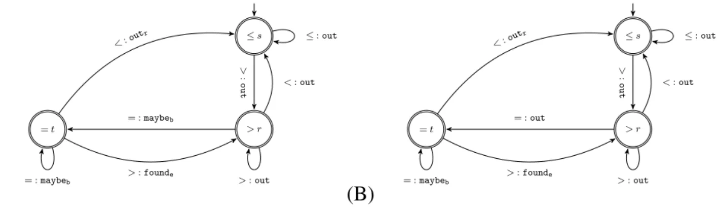
![Figure 5.3 – Register automata for NB _ PEAK and SUM _ WIDTH _ PEAK . These figures are adapted from [10].](https://thumb-eu.123doks.com/thumbv2/123doknet/11539550.295823/50.892.82.829.85.288/figure-register-automata-peak-width-peak-figures-adapted.webp)
![Table 7.3 – Classification of regular expressions: regular expression names σ, their properties and conditions on domain [`, u] when they hold.](https://thumb-eu.123doks.com/thumbv2/123doknet/11539550.295823/95.892.117.812.89.1129/table-classification-regular-expressions-regular-expression-properties-conditions.webp)
![Table 8.1 – For every regular expression σ, [`, u] is an integer interval domain, and n is a time series length, such that there is at least one ground time series of length n over [`, u] whose signature contains at least one occurrence of σ](https://thumb-eu.123doks.com/thumbv2/123doknet/11539550.295823/103.892.119.784.86.375/table-regular-expression-integer-interval-signature-contains-occurrence.webp)