HAL Id: hal-00482014
https://hal.archives-ouvertes.fr/hal-00482014
Submitted on 26 Nov 2012
HAL is a multi-disciplinary open access
archive for the deposit and dissemination of
sci-entific research documents, whether they are
pub-lished or not. The documents may come from
teaching and research institutions in France or
abroad, or from public or private research centers.
L’archive ouverte pluridisciplinaire HAL, est
destinée au dépôt et à la diffusion de documents
scientifiques de niveau recherche, publiés ou non,
émanant des établissements d’enseignement et de
recherche français ou étrangers, des laboratoires
publics ou privés.
Global propagation of side constraints for solving
over-constrained problems
Thierry Petit, Emmanuel Poder
To cite this version:
Thierry Petit, Emmanuel Poder. Global propagation of side constraints for solving over-constrained
problems. Annals of Operations Research, Springer Verlag, 2011, pp.20. �10.1007/s10479-010-0683-4�.
�hal-00482014�
(will be inserted by the editor)
Global propagation of side constraints for solving
over-constrained problems
An earlier publication of a shorter version of this paper (6 pages) has been published in the Lectures Notes in Computer Science series. The ISBN is 978-3-540-68154-0.
Thierry Petit · Emmanuel Poder
Received: date / Accepted: date
Abstract This article deals with the resolution of over-constrained problems using constraint programming, which often imposes to add to the constraint network new side constraints. These side constraints control how the initial constraints of the model should be satisfied or violated, to obtain solutions that have a practical interest. They are specific to each application. In our experiments, we show the superiority of a frame-work where side constraints are encoded by global constraints on new domain variables, which are directly included into the model. The case-study is a cumulative scheduling problem with over-loads. The objective is to minimize the total amount of over-loads. We augment the Cumulative global constraint of the constraint programming solver
Choco with sweep and task interval violation-based algorithms. We provide a theoretical
and experimental comparison of the two main approaches for encoding over-constrained problems with side constraints.
Keywords Constraint programming · Over-constrained problems · Cumulative
scheduling
1 Introduction
Constraint programming has been successfully used for solving industrial applications. For instance, each year, real-life problems solved with constraint programming tools are described in “applications papers”, in the proceedings of the international conference on
Principles and Practice of Constraint Programming [1]. Constraint programming was
also shown to be an effective alternative for solving hard pure combinatorial problems,
e.g., the maximum clique problem [2].
T. Petit ´
Ecole des Mines de Nantes, LINA UMR CNRS 6241
4 Rue Alfred Kastler, BP 20722, 44307 Nantes Cedex 3, FRANCE Tel.: +33 2 51 85 82 08
E-mail: [email protected] E. Poder
12 rue du Nil, 44470 Carquefou, FRANCE E-mail: [email protected]
Many industrial applications are defined by a set of constraints which are more or less important and cannot be all satisfied at the same time. Such problems are called over-constrained problems. Constraint programming systems should be able to provide as easily as possible an exploitable compromise when a problem has no solution satisfying all its constraints.
An usual way to deal with over-constrained problems is to turn a satisfaction prob-lem (without any solution) into a new optimization probprob-lem (with solutions): Viola-tions of constraints in the satisfaction problem are expressed through costs in the new problem. The goal is then to reduce the impact of violations of constraints of the ini-tial problem as much as possible. In this context, the foremost technique was parini-tial constraint satisfaction [3, 4].
In this article, we experiment this topic on a cumulative scheduling problem with human resource. The time unit is one hour and the schedule is also divided into days. We deal with the case where the scheduling horizon is fixed and not all activities can be scheduled with the available employees. In that case, over-loads can be accepted: at some points in time, it can be considered that extra-employees are available. To obtain solutions that have a practical interest, an usual requirement is to distribute over-loads as homogeneously as possible over a week. For instance, in a one week schedule, a user may impose that a solution where an over-load of 5 units of resource occurs on the first day is not an acceptable solution. However, he will accept a solution where this over-load of 5 units is distributed over 3 days. Note that different values are possible for a given violation, expressing a more or less important over-load. Another usual requirement is to express local dependencies between violations: “if constraint C1 is
violated then constraint C2 should not be violated”. For instance, a user may forbid
cumulating two neighbouring over-loads in two consecutive days: an over-load occurring the last hour of the first day, and another occurring the first hour of the second day.
These two classes of requirements are frequent in over-constrained problems. Many over-constrained problems impose to define new side constraints, to obtain solutions that satisfy such requirements. Although in many cases classical constraints can be used, e.g., in our case study the global cardinality constraint (Gcc) [5], specific global constraints based on statistics have been defined in [6, 7] to encode some requirements. A main use of these constraints is to model over-constrained problems. They may be used to obtain a balancing of values within a set of cost variables that represent violations. Gcc are used when the user needs to control the distribution of value in a more precise way, that is, explicitly by constraining the number of occurrences of cost values.
Our experiments compare the two usual generic frameworks for solving over-constrained problems as optimization problems. The first one extends constraint pro-gramming to handle violations as valuations [8]. User requirements are encoded by functions on violations. In the second framework [9], requirements are expressed by several global constraints, which communicate information on domains of possible val-ues of each violation. This framework imposes that violations are explicitly expressed by variables. The total sum of over-loads is minimized, to limit as much as possible unsatisfiability in solutions. In the two cases we used the same filtering technique for the relaxed version of the Cumulative constraint [10], which encodes the core of the problem, that is, the generic part, which is independent from side constraints. Side constraints are specific to each practical application.
Concretely, this paper provides three main contributions:
1. A model for a realistic cumulative over-constrained problem, where over-loads are tolerated according to some user requirements.
2. An extension of the Cumulative constraint of Choco [11] to over-constrained prob-lems, thanks to violation-based sweep and interval filtering algorithms.
3. Theoretical and experimental comparisons of the two usual frameworks for over-constrained optimization problems, in terms of solving : extending constraint pro-gramming [8], or using a variable-based model [9]. The comparison especially fo-cuses on side constraints used to get optimal solutions which have a practical in-terest.
This work is motivated by the third investigation. Since a variable based model provides domains for the costs, it is possible to propagate globally events on these domains. That is, to propagate the specific side constraints. This propagation is possible when costs are explicitly represented by new variables in the model. Our experimental results emphasize that using a variable-based model may be the adequate approach for solving practical problems that involve side constraints, provided these side constraints can be encoded through powerful global constraints of the solver.
Section 2 defines the cumulative over-constrained problem we consider. Section 3 presents the related work and the motivations of this paper. Section 4 presents our soft version of the Cumulative constraint and a comparison of the proposed filtering algorithms. Section 5 presents the experimental comparison of the two frameworks. Section 6 shows some extensions of the global constraint used for the generic core of our case-study, and discusses the future work so as to deal with precedence constraints in over-constrained cumulative scheduling problems.
2 Human resource cumulative scheduling
Scheduling problems consist of ordering some activities. In cumulative scheduling, each activity requires, for its execution, the availability of a certain amount of resource (renewable resource). Each activity has a release date (minimum starting time) and a due date (maximum ending time).
2.1 Description
Let D(x) = {min(D(x)), . . . , max(D(x))} denote the integer domain of variable x. Definition 1 Let A = {a1, . . . , an} denote a set of n non-preemptive activities. For
each a ∈ A,
– start[a] is the variable representing its starting point in time. – dur[a] is the variable representing its duration.
– end[a] ∈ end is the variable representing its ending point in time.
– res[a] is the variable representing the discrete amount of resource consumed by a, also denoted the height of a.
Within Constraint Programming toolkits, cumulative problems are encoded using the Cumulative global constraint [10, 12–15].
Definition 2 Consider one resource with a limit of capacity max capa and a set A of n activities. At each point in time t, the cumulated height (amount of consumed resource) htof the set of activities overlapping t is ht=Pa∈A,start[a]≤t<end[a]min(D(res[a])).
The Cumulative global constraint [10] enforces that: – C1: For each activity a ∈ A, start[a] + dur[a] = end[a]. – C2: At each point in time t, ht≤ max capa.
In this article, we deal with cumulative over-constrained problems that may require to be relaxed w.r.t. the resource capacity at some points in time, to obtain solutions. The maximum due date is strictly fixed to a given number of days, making some instances not satisfiable. Time unit is one hour. Each day contains 7 hours of work (to the first day corresponds hours 0 to 6, to the second day hours 7 to 13, etc.). n activities have to be planned. Duration of each activity is fixed, between 1 hour and 4 hours. All due dates are initially the scheduling horizon, and all release dates are 0. An activity consumes a fixed amount of resource: the number of persons required to perform it. This resource is upper-bounded by the total number ideal capa of employees. Given that either some extra-employees can be hired, or some activities can eventually be performed with smaller teams than the ones initially planned, if the problem has no solution then at certain points in time the resource can be greater than ideal capa. However, to remain feasible in practice, solutions should satisfy some requirements w.r.t. such over-loads. Some of them are generic:
1. At any point in time, an over-load should not exceed a given margin. 2. The total sum of over-loads should be reasonable (ideally minimum).
Some requirements are specific to each particular context. In our problem, the two following requirements should be satisfied by solutions.
3. At most 3 over-loaded hours within a day of 7 hours of work, and among them at most one over-load greater than 1 extra-employee.
4. In two consecutive days, if the last hour of work is over-loaded then the first hour of the next day should not be over-loaded.
If no solution exist with these requirements, this means that no solution acceptable in practice can be found.
2.2 Motivation for the use of constraint programming
One advantage of constraint programming for solving over-constrained applications is the ability to separate the generic part of the problem, that is, in our case require-ments 1. and 2. in section 2.1, from the specific side constraints, which depend on each applicative context, (e.g., requirements 3. and 4. in section 2.1). Thus, generically sim-ilar problems that differ in the specific side constraints applied may be encoded with classical constraint solvers thanks to the paradigm we propose in this paper. Adding a constraint to a given constraint programming model should not spoil the solving strength, except if its filtering algorithm has a prohibitive cost or if the solving process depends strongly on a search heuristic that would be disturbed by this new constraint. Nevertheless, when a new constraint is added to a given model, the number of solutions may drastically decrease. Therefore, propagation of side constraints has to be effective. This article aims to provide some answers w.r.t. the methodology that should be chosen to deal with this kind of over-constrained problems, which include side constraints.
3 Related work and Motivations
Using optimistic heuristics within a constraint system, researchers have studied large over-loaded cumulative problems without side constraints [16]. Baptiste et al. presented a soft global constraint for unsatisfiable one machine problems [17]. In the literature, one may find also some works about multi-objective relaxed time-tabling [18] expressed by constraint models.
More generally, when not all constraints can be satisfied, we search for a compromise solution which satisfies the constraints as much as possible. This is an optimization problem with a criterion on constraint violations. The goal is to find a solution which
best respects the set of initial constraints. In such a solution, hard constraints must be
satisfied, whereas soft constraints may be violated.
Side constraints can be used to precisely control violations of soft constraints. They specify solutions which have a practical interest, and eliminate the other ones. The objective of this article is to compare the approaches that can be used for solving over-constrained problems with side constraints.
3.1 Extending constraint programming
The first way to express an over-constrained problem is to extend constraint pro-gramming with an external structure, which handles relaxation of constraints [8]. The principle is to associate a valuation with each tuple of each constraint, which is null when satisfied. Thus, soft constraints are violation functions. Hard constraints have an “infinite” valuation for each violating tuple.
Valuations are aggregated into optimization criteria, to obtain a solution which best respects the soft constraints. Side constraints must be also expressed by objective criteria because violation costs are externalized from the constraint model.
3.2 Handling relaxation within the constraint programming framework
Instead of externalizing violation costs through functions, this approach consists of capturing violation costs through new variables in the problem [9]. Usually integer variables are used. Values in the domain of a violation variable express different degrees of violation (such domains are maintained by classical constraints).
Given a Constraint Satisfaction Problem (CSP), let X , D and C be respectively the set of variables, the set of domains and the set of constraints. When the CSP has no solution, C is split into two disjoint sets: the set Ch of hard constraints that must be
satisfied, and the set Csof soft constraints that may be violated.
The principle of the paradigm integrating violation costs through new variables is to turn the CSP1into a new constraint optimization problem. For each constraint in Cs, a new variable is defined. The set of these variables, denoted by costV ar, is
one-to-one mapped with Cs. To improve the solving efficiency, in many problems global
constraints can be used instead of a conjunction of more primitive constraints, and then several variables in costV ar can be included in the same global constraint. The
1 W.l.o.g., the initial over-constrained problem may be a constraint optimization problem.
In this case, the reformulation leads to a multi-criteria problem, with the original criterion plus a new criterion related to constraint violations.
new optimization problem imposes to satisfiy the set of hard constraints of the problem, possibly a set of new side constraints Side on costs (e.g., [6, 7]), which may be empty, and disjunctive constraints which integrate variables costV ar. This set of disjunctive constraints replaces the set Cs in the new constraint network we define. Let C ∈ Cs
be associated with a variable s ∈ costV ar. A value of s corresponds to a state of the constraint: if s = 0 then C is satisfied, and if s > 0 then C is violated. That is, the disjunctive constraint is [C ∧ [s = 0]] ∨ [¬C ∧ [s > 0]].
For sake of efficiency, expression [¬C ∧ [s > 0]] is, in practice, expressed by a constraint sof tC ∈ Sof t integrating variables of C and the cost variable s in Cs. The
disjunctive constraint is then [C ∧ [s = 0]] ∨ sof tC, or even simply sof tC. The interest is to better take into account the semantics so as to improve the pruning efficiency.
In this case, the filtering algorithm of the global soft constraint should implement the filtering algorithm of C for the case s = 0. Such a constraint is called a soft global
constraint [19, 20].
Optimization criteria are related to the whole set of variables in costV ar. Strictly positive values of variables costV ar semantically correspond to violations of initial constraints in Cs. Hence, the intial CSP is turn into a new optimization problem hX ∪
costV ar, D ∪ DcostV ar, Ch∪ Sof t ∪ Sidei.
Compared with the paradigm presented in section 3.1, one main difference is the possibillity to propagate some side constraints on cost variables, which is not possible if the problem does not include explicitely cost variables.
3.3 Propagation of side constraints
The use of extra-variables to express violations does not entail any solving penalty when domains of possible values for violations are reduced monotonically during search. In-deed, algorithms dedicated to valuation-based frameworks can be used with violation variables. Furthermore, all search heuristics used with valuation-based paradigms [8] can be used in variable-based paradigms [9]. In this case, all violation variables will have a value by propagation. Branching is performed only on problem variables. Thus, we can obtain the same search tree with variable and valuation-based frameworks if the same filtering algorithms are used. The advantage of using variables instead of cost functions is to propagate globally external constraints on these variables (the central topic of this article), and also to benefit from propagation of events on violation vari-ables in both directions (from the objective to the varivari-ables and vice versa).
For sake of modelling, two existing solving techniques specific to valuation-based frameworks would require some research effort to be suited to our case-study.
In the first one, solving is performed by variable elimination [21]. This algorithm is currently not suited to global n-ary constraints as Cumulative or its extensions.
In the second one, to improve the pruning power valuations are projected from tu-ples to values and vice versa [22]. Domains of possible values for violations are reduced monotonically during search. This approach is effective for some problems without side constraints, when good global lower bounds can be obtained by an aggregation of local costs. However, if valuations can increase and decrease (they do not express over-loads), defining and propagating side constraints such as Gcc [5], Spread [6] or Deviation [7], or sets of side constraints expressing dependencies between constraint violations, is not obvious, especially through an objective function. This point represents a future
Valuations (cost functions)
Violation variables
Core of the problem
(e.g., global soft constraint) (e.g., global soft constraint)
Core of the problem
Optimization Criteria
Valued Model
Optimization Criteria
Variable−based Model
expressing also side constraints
Global constraints that express side contraints
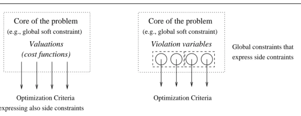
Fig. 1 With a variable-based model, a global propagation can be performed on violation variables through side constraints, which is not the case with a valuation-based approach because violations are not expressed by variables.
research direction with respect to such solving techniques, which is out of the scope of this paper.
Additionally to a global soft constraint expressing the core of the over-constrained problem, our goal is to investigate whether propagating globally some side constraints improves the solving process or not. Note that a comparison of the variable-based and valuation-based approaches in terms of modelling was performed in [9].
These external side constraints depend on each specific problem, e.g, rules 3. and 4. in section 2. As depicted by Figure 1, with a valuation-based encoding, side constraints can be expressed by the optimization function. No domains are available for violations, which are evaluated externally through functions. Conversely, with a variable-based encoding, it is possible to use global constraints on violation variables.
4 Cumulative Constraint with Over-Loads
This section presents the SoftCumulativeSum constraint, useful to express our case-study and deal with significant instances.
4.1 State of the Art : Pruning Independent from Relaxation
The SoftCumulativeSum constraint that will be presented in Section 4.2 implicitly defines a Cumulative constraint with a capacity equal to max capa. To prune variables in start, several existing algorithms for Cumulative can be used. We recall the two filtering techniques currently implemented in the Cumulative of Choco solver [11], which we extend to handle violations in section 4.2.
4.1.1 Sweep Algorithm [14]
The goal is to reduce domains of start variables according to the cumulated profile, which is built from compulsory parts of activities, in order not to exceed max capa.
This is done in Choco using a sweep algorithm [14]. The Compulsory Part [23] of an activity is the intersection of all feasible schedules of the activity.2 As the domains of the variables of the activity get more and more restricted, the compulsory part will increase until becoming a schedule of the activity.
It is equal to the intersection of the two particular schedules that are the activity scheduled at its latest start and the activity scheduled at its earliest start. As domains of variables get more and more restricted, the compulsory part increases, until it becomes the fixed activity.
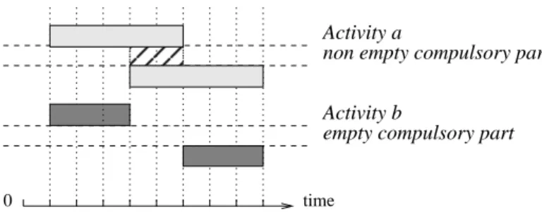
Definition 3 The Compulsory Part CP (a) of an activity a is not empty if and only if max(D(start[a])) < min(D(end[a])). If so, its height is equal to min(D(res[a])) on [max(D(start[a])), min(D(end[a]))[ and null elsewhere.
time 0
non empty compulsory part
empty compulsory part Activity a
Activity b
Fig. 2 Compulsory parts.
Example 1 Let a be an activity such that start[a] ∈ [1, 4], with a duration fixed to 5,
and b be an activity such that start[b] ∈ [1, 6], with a duration fixed to 3. As depicted by Figure 2, activity a has a non empty compulsory part, while activity b has an empty compulsory part.
Definition 4 The Cumulated Profile CumP is the minimum cumulated resource
con-sumption, over time, of all the activities. For a given t, the height of CumP at time t
is equal to X
a∈A/t∈[max(D(start[a])),min(D(end[a]))[
D(min(res[a]))
That is, the sum of the contributions of all compulsory parts that overlap t.
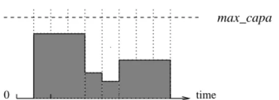
The next figure shows an example of a cumulative profile CumP where at each point in time t the height of CumP at t does not exceed max capa.
Algorithm The sweep algorithm moves a vertical line ∆ on the time axis from one
event to the next event. In one sweep, it builds the cumulated profile incrementally and prunes activities according to this profile, in order not to exceed max capa. An event corresponds either to the start or the end of a compulsory part, or to the release date of
2 Therefore, it is sufficient, in the computation of the compulsory part of an activity a,
to consider only its feasible schedule with duration and resource consumption fixed at their minimum.
time 0
max_capa
Fig. 3 Cumulated profile.
an activity. All events are initially computed and sorted in increasing order according to their date. Position of ∆ is δ. At each step of the algorithm, a list ActT oP rune contains the activities to prune.
– Compulsory part events are used for building CumP . All events at date δ are used to update the height sumh of the current rectangle in CumP : if such an event
corresponds to the start (respectively to the end) of a compulsory part then the height of this compulsory part is added to (resp. subtracted from) sumh. The first
event with a date strictly greater than δ gives the end δ′ of the current rectangle in CumP , denoted by h[δ, δ′[, sumhi.
– Events corresponding to release dates d such that δ ≤ d < δ′ add some new activities to prune, according to h[δ, δ′[, sumhi and max capa (those activities which
overlap h[δ, δ′[, sumhi). They are added to the list ActT oP rune.
For each a ∈ ActT oP rune that has no compulsory part registered in the rectangle h[δ, δ′[, sumhi, if its height is greater than max capa − sumhthen the algorithm prunes
its start time so this activity doesn’t overlap the current rectangle of CumP . Then, if the due date of a is less than or equal to δ′then a is removed from ActT oP rune. After pruning activities, δ is updated to δ′.
Pruning Rule 1 Let a ∈ ActT oP rune, which has no compulsory part recorded
within the rectangle h[δ, δ′[, sumhi. If sumh + min(D(res[a])) > max capa then
]δ − min(D(dur[a])), δ′[ can be removed from D(start[a]).
Time complexity of the sweep technique is O(n ∗ log(n)). Please refer to the paper for more details w.r.t. this algorithm [14].
4.1.2 Energy reasoning on Task Intervals [24, 12, 25]
The principle of energy reasoning is to compare the resource necessarily required by a set of activities within a given interval of points in time with the available resource within this interval. Relevant intervals are obtained from starts and ends of activities (“task intervals”). This section presents the rules implemented in Choco.
Notation 1 Given ai and aj two activities (possibly the same) s.t.
min(D(start[ai])) < max(D(end[aj])), we denote by:
– I(ai,aj)the interval [min(D(start[ai])), max(D(end[aj]))[.
– S(ai,aj) the set of activities whose time-windows intersect I(ai,aj) and such that
their earliest start is in I(ai,aj), that is, S(ai,aj)= {a ∈ A s.t. min(D(start[ai])) ≤
min(D(start[a])) < max(D(end[aj]))}.
– Area(ai,aj) the number of free resource units in I(ai,aj), that is, Area(ai,aj) = (max(D(end[aj])) − min(D(start[ai]))) ∗ max capa.
Definition 5 A lower bound W(ai,aj)(a) of the number of resource units consumed
by a ∈ S(ai,aj)on I(ai,aj)is
W(ai,aj)(a)
=
min(D(res[a])) ∗ min[min(D(dur[a])), max(0, max(D(end[aj])) − max(D(start[a])))]
Feasibility Rule 1 IfPa∈S
(ai,aj )W(ai,aj)(a) > Area(ai,aj)then fail.
Algorithm The principle is to browse, by increasing due date, activities aj ∈ A and
for a given aj to browse, by decreasing release date, activities ai ∈ A such that
min(D(start[ai])) < max(D(end[aj])). Hence, at each new choice of ai or aj more
activities are considered. For each couple (ai, aj), the algorithm applies the feasibility
rule 1.
Suppose the activities sorted by increasing release date i.e. min(D(start[a1])) ≤
min(D(start[a2])) ≤ · · · ≤ min(D(start[an])), then:
– If min(D(start[ai−1])) = min(D(start[ai])) then
S(a
i−1,aj) = S(ai,aj) and therefore
P
a∈S(ai−1,aj )W(ai−1,aj)(a) =
P
a∈S(ai,aj )W(ai−1,aj)(a). 3
– Else
We have S(ai−1,aj) = S(ai,aj) ∪ {ak ∈ A, k ≤ i − 1 ∧ min(D(start[ak])) =
min(D(start[ai−1]))} i.e. we add all activities with same release date than
activity ai−1. Hence, Pa∈S(ai−1,aj )W(ai−1,aj)(a) =
P
a∈S(ai,aj )W(ai,aj)(a) +
P
{k≤i−1∧min(D(start[ak]))=min(D(start[ai−1]))}W(ai,aj)(a).
Therefore, the complexity for handling all intervals I(ai,aj)is O(n2).
4.2 Pruning Related to Relaxation
Specific constraints on over-loads exist in real-world applications, e.g., rules 3. and 4. in Section 2. To express them, it is mandatory to discretize time, while keeping a reasonable time complexity for pruning. These specific constraints are externalized be-cause they are ad-hoc to each application. On the other hand, the following constraints capture the generic core of this class of problems.
– SoftCumulativeextends Cumulative of Choco by maintaining over-load variables at each point in time, and by pruning activities according to maximal available capacities given by upper bounds of these variables instead of simply considering max capa. This constraint can be used with various objective criteria.
– The SoftCumulativeSum extends the SoftCumulative. It is defined to deal more efficiently with a particular criterion: minimize the sum of over-loads.
3 By definition, W
4.2.1 SoftCumulative Constraint
Definition 6 Let A be a set of activities scheduled between time 0 and m, each
consuming a positive amount of the resource. SoftCumulative augments Cumulative with a second limit of resource ideal capa ≤ max capa, and for each point in time t < m an integer variable costV ar[t]. It enforces:
– C1 and C2 (see Definition 2).
– C3: For each point in time t, costV ar[t] = max(0, ht− ideal capa)
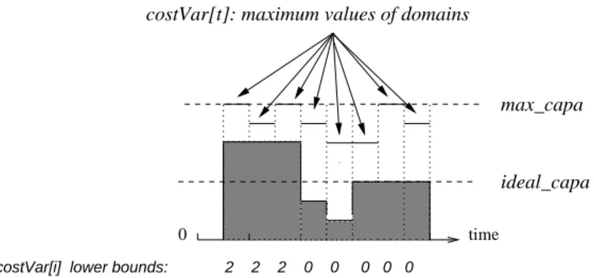
costVar[i] lower bounds: 2 2 2 0 0 0 0 0 0
ideal_capa max_capa costVar[t]: maximum values of domains
time
Fig. 4 Example of a SoftCumulative constraint.
Example 2 Figure 4 depicts an example of a cumulative profile CumP where at each
point in time t the height of CumP at t does not exceed the maximum value in the domain of its corresponding violation variable costV ar[t]. Points in time 1, 2, and 3 are such that CumP exceeds ideal capa by two. Therefore, for each point, the minimum value of the domain of the corresponding variable in costV ar should be updated to value 2.
Next paragraph details how the classical sweep procedure can be adapted to the SoftCumulativeconstraint.
Revised Sweep pruning procedure. The limit of resource is not max capa as in the
Cumulativeconstraint. It is mandatory to take into account upper-bounds of variables in costV ar. One may integrate reductions on upper bounds within the profile, as new fixed activities. However, our discretization of time can be very costly with this method: the number of events may grow significantly. The profile would not be computed only from activities but also from each point in time.
We propose a relaxed version where for each rectangle we consider the maximum costV ar upper bound. This entails less pruning but the complexity is amortized: the number of time points checked to obtain maximum costV ar upper bounds for the whole profile is m, by exploiting the sort on events into the sweep procedure.
The pruning rule 2 reduces domains of start variables from the current maximum allowed over-load in a rectangle.4
Pruning Rule 2 Let a ∈ ActT oP rune, which has no compulsory part recorded
within the current rectangle. If sumh + min(D(res[a])) > ideal capa +
maxt∈[δ,δ′[(max(D(costV ar[t]))) then ]δ − min(D(dur[a])), δ′[ can be removed from
D(start[a]).
Proof: For any activity which overlaps the rectangle, the maximum capacity is upper-bounded by ideal capa + max(D(costV ar[t]), t ∈ [δ, δ′[).
Time complexity is O(n ∗ log(n) + m), where m is the maximum due date.
Revised task Intervals energy reasoning. This paragraph describes the extension of the
principle of section 4.1.2 to the SoftCumulative global constraint. Feasibility Rule 2 Area(ai,aj)=
X
t∈[min(D(start[ai])),max(D(end[aj]))[
ideal capa + max(D(costV ar[t]))
IfPa∈S
(ai,aj )W(ai,aj)(a) > Area(ai,aj) then fail.
Proof: At each time point t there is ideal capa + max(D(costV ar[t])) available units.
Efficiency of rule 1 can be improved by this new computation of Area(ai,aj)(the
pre-vious value was an over-estimation). Since activities ai are considered by decreasing
release date, it is possible to compute incrementally Area(ai,aj). Each upper bound of a variable in costV ar are considered once for each aj. Time complexity is O(n2+n∗m),
where m is the maximum due date.
Next paragraph explains how minimum values of domains of variables in costV ar are updated during the search process.
Update costVar lower-bounds. Update of costV ar lower bounds can be directly
per-formed within the sweep algorithm, while the profile is computed.
Pruning Rule 3 Consider the current rectangle in the profile, [δ, δ′[. For each t ∈ [δ, δ′[, if sumh− ideal capa > min(D(costV ar[t])) then [min(D(costV ar[t])), sumh−
ideal capa[ can be removed from D(costV ar[t]).
Proof: From Definitions 3 and 4.
Usually the constraint should not be associated with a search heuristic that forces to assign to a given variable in costV ar a value which is greater than the current lower bound of its domain. Indeed, such a search strategy would consist of imposing at this point in time a violation although solutions with lower over-loads at this point in time
4 The upper bound max(D(costV ar[t])) is the maximum value in the domain D(costV ar[t]).
Since these variables may be involved in several constraints, especially side constraints, the maximum value of a domain can be reduced during the search process.
exist (or even solutions with no over-load). However, it is required to take into account this eventuality and to ensure that our constraint is valid with any search heuristic. If a greater value is fixed to a variable in costV ar, until more than a very few unfixed activities exist, few deductions can be made in terms of pruning and they may be costly (for a quite useless feature). Therefore, we implemented a check procedure that fails when all start variables are fixed and one variable in costV ar is higher than the current profile at this point in time. This guarantees that ground solutions will satisfy the constraint in any case, with a constant time complexity.
4.2.2 SoftCumulativeSum Constraint
Definition 7 SoftCumulativeSumaugments SoftCumulative with an integer variable cost. It enforces:
– C1 and C2 (see Definition 2), and C3 (see Definition 6). – The following constraint: cost =Pt∈{0,...,m−1}costV ar[t]
Pruning procedures and consistency checks of SoftCumulative remain valid for SoftCumulativeSum. Additionally, we aim at dealing with the sum constraint efficiently by exploiting the semantics. We compute lower bounds of the sum expressed by cost variable. Classical back-propagation of this variable can be additionally performed as if the sum constraint was defined separately.
Example 3 The term back-propagation is used to recall that propagation of events
is not only performed from the decision variables to the objective variable but also from the objective variable to decision variables. For instance, let x1, x2 and x3 be
3 variables with the same domain: ∀i ∈ {1, 2, 3}, D(xi) = {1, 2, 3}. Let sum be a
variable, D(sum) = {3, 4, . . . , 9}, and the following constraint sum = Pi∈{1,2,3}xi.
Assume that 2 is removed from all D(xi). The usual propagation removes values 4, 6
and 8 from D(sum). Assume now that all values greater than or equal to 5 are removed from D(sum). Back-propagation removes value 3 from all D(xi).
Sweep based global lower bound. Within our global constraint, a lower bound for the
cost variable is directly given by summing the lower bounds of all variables in costV ar, which are obtained by pruning rule 3. These minimum values of domains were computed from compulsory parts, not only from fixed activities.
LB1=
X
t∈{0,...,m−1}
min(D(costV ar[t]))
LB1can be computed with no increase in complexity within the sweep algorithm.
Interval based global lower bound. The quantity Pa∈S
(ai,aj )W(ai,aj)(a) used in
fea-sibility rule 1 provides the required energy for activities in the interval I(ai,aj). This
quantity may exceed the number of time points in I(ai,aj) multiplied by ideal capa.
We can improve LB1, provided we remove from the computation over-loads already
taken into account in the cost variable. In our implementation, we first update variables in costV ar (by rule 3), and compute LB1 to update cost. In this way, no additional
incremental data structure is required.
To obtain the new lower bound we need to compute lower-bounds of cost which are local to each interval I(ai,aj).
Definition 8 lb1(ai,aj)=
P
t∈I(ai,aj )min(D(costV ar[t]))
Then, next proposition is related to the free available number of resource units within a given interval.
Proposition 1 The number FreeArea(ai,aj) of free resource units in I(ai,aj) s. t. no violation is entailed is (max(D(end[aj])) − min(D(start[ai]))) ∗ ideal capa.
Proof: From Definition 7.
From Definition 8 and Proposition 1, FreeArea(ai,aj)+ lb1(ai,aj)is the number of time units that can be used without creating any new over-load into the interval I(ai,aj)compared with over-loads yet taken into account in lb1(ai,aj).
Definition 9 Inc(ai,aj)=
P
a∈S(ai,aj )W(ai,aj)(a)−FreeArea(ai,aj)− lb1(ai,aj)
Inc(a
i,aj)is the difference between the required energy and this quantity. Even if one
variable in costV ar has a current lower bound higher that the value obtained from the profile, the increase Inc(ai,aj) is valid (smaller, see Definition 8). We are now able to improve LB1.
LB2= LB1+ max(ai,aj)∈A2(Inc(ai,aj))
Another lower bound can be computed from a partition P of [0, m[ in disjoint intervals obtained from pairs of activities (ai, aj): LB(P )= LB1+PI(ai,aj )∈P Inc(ai,aj).
Ob-viousy LB2≤ LB(P ). However, time complexity of the algorithm deduced from rule 2
in the SoftCumulative constraint is O(n2+ n ∗ m). Computing LB(P )would increase
this complexity.5Conversely, it is straightforward that computing LB2can be directly
performed into this algorithm without any increase in complexity.
Pruning Rule 4 If LB2 > min(D(cost)) then [min(D(cost)), LB2[ can be removed
from D(cost).
Proof: From Definition 7, LB1is a lower bound of cost. Since intervals are disjoint, by
Defi-nition 9 the quantity LB(P )is a lower bound of cost. LB2≤LB(P ). Therefore LB2is a lower
bound of cost. The pruning rule holds.
Aggregating local violations. Once the profile is computed, if some activities having a
null compulsory part cannot be scheduled without creating new over-loads, then LB1
can be augmented with the sum of minimum increase of each activity. This idea is inspired from generic solving methods for over-constrained CSPs, e.g., Max-CSP [26]. Our experiments shown that there is quite often a way to place any activity without creating a new violation. This entails a null lower bound. Therefore, we removed that computation from our implementation. We inform the reader that we described the procedure in a preliminary technical report [27].
4.2.3 Implementation
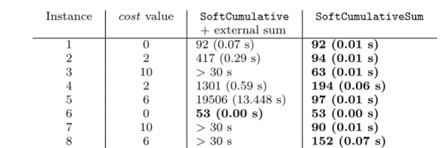
Constraints were implemented (using Choco) to work with non fixed durations and Table 1 compares the two constraints on small problems when the objective is to minimize cost. Results show the main importance of LB2 when minimizing cost.
5 Determining a relevant partition P from the activities would force to use an independent
algorithm, which can be costly depending on the partition we search for. Finally, we decided to use only LB2.
Instance costvalue SoftCumulative SoftCumulativeSum + external sum 1 0 92 (0.07 s) 92 (0.01 s) 2 2 417 (0.29 s) 94 (0.01 s) 3 10 >30 s 63 (0.01 s) 4 2 1301 (0.59 s) 194 (0.06 s) 5 6 19506 (13.448 s) 97 (0.01 s) 6 0 53 (0.00 s) 53 (0.00 s) 7 10 >30 s 90 (0.01 s) 8 6 >30 s 152 (0.07 s)
Table 1 Number of nodes required to find optimum schedules with n = 9, m = 9, durations between 1 and 4, resource consumption between 1 and 3, ideal capa = 3, max capa = 7.
5 Variable-Based vs Valuation-Based Model 5.1 Definition of the Constraint Network
Within the context of a practical application, the goal of this article is to compare frameworks for solving over-constrained problems : extending constraint programming [8], or using a variable-based model [9]. Here is the variable based model in a pseudo-code syntax. Comments show how rules on violations of Section 2 are expressed.
int[] ds, hs; // fixed random durations and heights int ideal capa, max capa;
IntDomainVar[] start, costVar; IntDomainVar cost; // core of the problem
SoftCumulativeSum(start, costVar, cost, ds, hs, ideal capa, max capa); // side constraints
for each array "day", element of a partition of costVar[]: Gcc6 ("day",...)); // rule 3 (max 3 over-loads) AtMostKNotZeroOrOne("day",1)); // rule 3 (max 1 big over-load) for(i:7..costVar.length-1): // rule 4 (consecutive days)
if(i%7==0): [costVar[i-1]==0 || costVar[i]==0]; // objective criteria
minimize(cost)
A disjunction is sufficient for expressing rule 4. because, given a pair of variables, the constraint just consists of forcing to assign value 0 to one of the two variables when value 0 is removed from the other one. For more complex dependencies, a Regular constraint may be used to improve the solving efficiency [28].
The ad-hoc constraint AtMostKNotZeroOrOne imposes to have at most k times val-ues different from 0 or 1 into a set of variables which is given as argument.
Provided domains of costs are monotonically reduced (which is mandatory for mod-elling our case-study with the side constraints, see section 3.3), all algorithms used with
6 Global Cardinality Constraint, also called Distribute [5]. Given a set of variables (here,
a day of 7 point in times), this constraint specifies for each possible value v in the union of variable domains the minimum and maximum number of times v can be assigned to a variable. Here, to value 0 (no over-load) corresponds the range [4, 7] (at least 4 times), to value 1 corresponds [0, 3], and to any value strictly greater than 1 corresponds [0, 1].
a valuation-based framework can be used with a variable based framework so as to ob-tain exactly the same search tree [9]. Reciprocally, to reproduce the filtering algorithms of our global constraint using a valuation-based solver, one may build a solver dedi-cated to this class of problems. Hence, concerning the generic part of the problem, the two frameworks are equivalent.
Conversely, to encode specific rules of our case-study (rules 3. and 4.) with a valuation-based model, it is necessary to encode the Gcc’s plus a set of dependen-cies plus a sum constraint through an optimization criterion, to select the acceptable solutions of the problem. We are not aware of a paper providing a technique to define and to implement such a optimization criterion. Implementing such a criterion would certainly be a scientific contribution. Nevertheless, we do not claim that it is not pos-sible, and we assume that our problem can be expressed in both cases.
Assuming that it is possible, there is still a significant difference between the two frameworks. In a variable-based framework a global propagation of value deletions in the domains of costs can be performed (because costs are represented by variables), and in a valued framework it is not possible (because no domains are available for the costs). Such a global propagation is performed through side constraints whose semantics are specific to the practical problem we consider. These semantics can be exploited by filtering algorithms of side constraints, to improve their pruning efficiency. We can simulate a valuation-based encoding with a particular variable-based model. We disconnect global pruning algorithms of side constraints, which are transformed into constraint checkers. Indeed, a valuation-based model express violations by functions that, given a tuple, return a valuation. Valuations are aggregated into the objective criterion. Side constraints 3. and 4. eliminate assignments that do not respect rules that should be necessarily satisfied by solutions. Thus, when expressing rules by an objective criterion, this objective criterion has to reject the wrong assignments. This behaviour can be simulated by implementing constraints that do not propagate globally on violation variables but just answer ’yes’ or ’no’ given a (possibly partial) assignment. Hence, we used consistency checkers for encoding side constraints, instead of complete side constraints with a filtering algorithm. The valuations corresponding to a partial or a complete assignment are then the lower bounds of variables in costV ar. We call the modified constraints NFGcc and NFAtMostKNotZeroOrOne. Except these modified side constraints, the two models are exactly the same, notably w.r.t. the SoftCumulativeSum constraint and its filtering algorithm.
5.2 Experiments
Benchmarks were generated randomly with seeds to be reproducible. They were run with the same search heuristic: assign minimum values of domains first to start variables and after to costV ar and cost variables. This search heuristic is consistent with a valuation-based model. There is no branching on cost variables. The machine was a 2.2 Ghz Intel Core 2 processor with 4 Go of 667 Mhz RAM.
Table 2 shows that even for small instances of our case-study, expressing side con-straints as functions is not well suited to avoid a high number of nodes. Conversely, using the variable-based model leads to a robust solving.
Instance costvalue Valuation-based Model Variable-based Model 1 0 67 (0.08 s) 67 (0.01 s) 2 0 3151 (6.07 s) 74 (0.02 s) 3 5 372 (0.6 s) 117 (0.1 s) 4 0 2682 (4.4 s) 120 (0.03 s) 5 4 116 (0.1 s) 134 (0.1 s) 6 0 62 (0.01 s) 132 (0.04 s) 7 10 1796 (2.3 s) 694 (0.9 s) 8 4 391 (0.48 s) 352 (0.45 s)
Table 2 Number of nodes required to find optimum schedules with n = 10, m = 14, dura-tions between 1 and 4, resource consumption between 1 and 3, ideal capa = 3, max capa = 7.
Instance costvalue Valuation-based Model Variable-based Model
1 2 >60 s 211 (0.34 s) 2 0 >60 s 178 (0.08 s) 3 1 >60 s 200 (0.12 s) 4 15 >60 s 27 (0.04 s) 5 12 >60 s 546 (2 s) 6 3 >60 s 1875 (6 s) 7 6 2240 (11.4 s) 160 (0.12 s) 8 9 >60 s 79 (0.06 s)
Table 3 Number of nodes required to find optimum schedules with n = 15, m = 21, dura-tions between 1 and 4, resource consumption between 1 and 3, ideal capa = 3, max capa = 7.
Instance costvalue Variable-based Model
1 3 858 (5.8 s) 2 0 627 (1.2 s) 3 - >60 s 4 0 419 (0.6 s) 5 - >60 s 6 23 263 (1.6 s) 7 10 416 (0.9 s) 8 19 197 (0.6 s)
Table 4 Number of nodes required to find optimum one week schedules: n = 25, m = 35, durations between 1 and 4, resource consumption between 1 and 3, ideal capa = 3, max capa = 7.
Table 3 confirms the superiority of a variable-based model. However, some instances (e.g., 6 in this table) can involve more than one thousand nodes with the variable-based model. This fact shows that some hard instances remain despite the efficient handling of over-load distribution.
We aim to determine whether the variable model may solve a schedule of one week. Table 4 shows that some instances cannot be solved within a time less than 60 s. This is partially due to the time spent into the SoftCumulativeSum constraint at each node, which grows proportionally to the number of variables although we did not integrate time points as events into the sweep pruning procedure.
6 Extensions and future work
We presented case-study where propagating side constraints is mandatory for solving the instances. We presented a global constraint for the generic part of this case-study. This global constraint can be tailored to suited to some other classes of applications.
6.1 Lightened relaxation
If the time unit is tiny compared with the scheduling horizon, e.g., one minute in a one-year schedule, the same kind of model may be used by grouping time points. For example, each violation variable may correspond to one half-day. Imposing a side constraint between two particular minutes into a one-year schedule is generally not useful. For this purpose, the SoftCumulative constraint can be generalized, to be relaxed with respect to its number of violation cost variables.
6.1.1 RelSoftCumulative constraint
Notation 2 To define RelSoftCumulative we use the following notations. Given a
set of activities scheduled between 0 and m,
– mult ∈ {1, 2, ..., m} is a positive integer multiplier of the unit of time.
– Starting from 0, the number of consecutive discrete intervals of length mult that are included in the interval [0, ..m[ is ⌈m/mult⌉. J = {0, 1, . . . , ⌈m/mult⌉ − 1} is the set of indexes of such intervals. Hence, to each j ∈ J corresponds the interval
[j ∗ mult, j ∗ mult + 1, . . . (j + 1) ∗ mult − 1].
Definition 10 Let A be a set of activities scheduled between time 0 and m, each con-suming a positive amount of the resource. RelSoftCumulative augments Cumulative with
– A second limit of resource ideal capa ≤ max capa, – The multiplier mult ∈ {1, 2, . . . , m},
– For each j ∈ J an integer variable costV ar[j]. It enforces:
– C1 and C2 (see Definition 2).
– C4: For each j ∈ J , costV ar[j] =P(j+1)∗mult−1t=j∗mult max(0, ht− ideal capa)
Example 4 We consider a cumulative over-constrained problem with n activities
sched-uled minute by minute over one week. The scheduling horizon is m = 2940. Assume that a user formulates a side constraint related to the distribution of over-loads of resource among ranges of one hour (mult = 60) in the schedule, for instance ”no more than one hour violated each half-day”. The instance of RelSoftCumulative related to this problem is defined with ⌈2940/60⌉, i.e., 49 violation variables, J = {0, 1, . . . , 48}. For each range indexed by j ∈ J , the constraint C3 is: costV ar[j] = sum(j+1)∗60−1t=j∗60 max(0, ht− ideal capa). The side constraint is then simply expressed
by cardinality constraints over each half-day, that is, each quadruplet of violation vari-ables: {costV ar[0], · · · , costV ar[3]}, {costV ar[4], · · · , costV ar[7]}, etc.
6.1.2 RelSoftCumulativeSum constraint
Definition 11 RelSoftCumulativeSumaugments RelSoftCumulative with an integer
variable cost. It enforces:
– C1 and C2 (see Definition 2), and C4 (see Definition 10). – The following constraint: cost =Pj∈JcostV ar[j]
6.1.3 Pruning algrithms
It is straightforward to reformulate rules of section 4.2 to make them suited to RelSoftCumulative. With respect to RelSoftCumulativeSum, the sweep based global lower bound computation is identical to the one of the SoftCumulativeSum. The interval based global lower bound of SoftCumulativeSum can be also adapted to RelSoftCumulativeSum; the task interval energetic reasoning presented in section 4.2.2 differs by the evaluation of the quantity lb1. We presented the details in a technical
note (see [29]). A perspective of our article will be to evaluate the pruning power of these extensions and to compare them with some alternative models. For instance, it may be possible to state several copies of the SoftCumulative constraint at different time scales on clones of the resources (with the coarser resources kept synchronized with the finer ones through channeling constraints).
6.2 Precedence constraints and violation criteria
Some scheduling problems include precedence constraints. We will investigate whether integrating precedence constraints into an energetic reasoning is of interest or not in the context of over-constrained problems, compared with the case where the prece-dence graph is handled separately from the SoftCumulativeSum constraint or from the RelSoftCumulativeSum constraint. More generally, our future work will consists of determining which parts of these problems should be relaxed (precedence constraints, over-loads of resource, or both precedence constraints and over-loads), according to the different classes of applications, and providing answers to the related algorithmic issues. Moreover, in some applications violating a fixed scheduling horizon could be interesting.
7 Conclusion
This paper analyzed the benefit of propagating a set of global constraints on viola-tions variables, in terms of solving efficiency. To encode the case-study we selected for these experiments, we proposed several filtering procedures for a global Cumulative constraint which is relaxed w.r.t. to its capacity at some points in time. Experiments demonstrated that its own filtering is not sufficient. Propagating globally additional constraints on violation variables is required. At last, we provided the extension of our global constraint for the case where side constraints are related to ranges in time which are larger than one time unit.
References
1. Stuckey, P.J. (ed.): Principles and Practice of Constraint Programming, 14th International Conference, CP 2008, Sydney, Australia, September 14-18, 2008. Proceedings, Lecture Notes in Computer Science, vol. 5202. Springer (2008)
2. R´egin, J.C.: Using constraint programming to solve the maximum clique problem. Proc. CP pp. 634–648 (2003)
3. Freuder, E.: Partial constraint satisfaction. Proc. IJCAI pp. 278–283 (1989)
4. Freuder, E., Wallace, R.: Partial constraint satisfaction. Artificial Intelligence 58, 21–70 (1992)
5. R´egin, J.C.: Generalized arc consistency for global cardinality constraint. Proc. AAAI pp. 209–215 (1996)
6. Pesant, G., R´egin, J.C.: Spread: A balancing constraint based on statistics. Proc. CP pp. 460–474 (2005)
7. Schaus, P., Deville, Y., Dupont, P., R´egin, J.C.: The deviation constraint. Proc. CPAIOR pp. 260–274 (2007)
8. Bistarelli, S., Montanari, U., Rossi, F., Schiex, T., Verfaillie, G., Fargier, H.: Semiring-based CSPs and valued CSPs: Frameworks, properties, and comparison. Constraints 4, 199–240 (1999)
9. Petit, T., R´egin, J.C., Bessi`ere, C.: Meta constraints on violations for over constrained problems. Proc. IEEE-ICTAI pp. 358–365 (2000)
10. Aggoun, A., Beldiceanu, N.: Extending CHIP in order to solve complex scheduling and placement problems. Mathl. Comput. Modelling 17(7), 57–73 (1993)
11. Choco: An open source Java CP library, documentation manual. http://choco.emn.fr/ (2009)
12. Caseau, Y., Laburthe, F.: Cumulative scheduling with task intervals. Proc. JICSLP (Joint International Conference and Symposium on Logic Programming) pp. 363–377 (1996) 13. Carlsson, M., Ottosson, G., Carlson, B.: An open-ended finite domain constraint solver.
Proc. PLILP pp. 191–206 (1997)
14. Beldiceanu, N., Carlsson, M.: A new multi-resource cumulatives constraint with negative heights. Proc. CP pp. 63–79 (2002)
15. Mercier, L., Hentenryck, P.V.: Edge finding for cumulative scheduling. INFORMS Journal on Computing 20(1), 143–153 (2008)
16. Benoist, T., Jeanjean, A., Rochart, G., Cambazard, H., Grellier, E., Jussien, N.: Subcon-tractors scheduling on residential buildings construction sites. ISS’06 Int. Sched. Sympo-sium, Technical Report JSME-06-203 pp. 32–37 (2006)
17. Baptiste, P., Pape, C.L., Peridy, L.: Global constraints for partial CSPs: A case-study of resource and due date constraints. Proc. CP pp. 87–102 (1998)
18. Rudov´a, H., Vlk, M.: Multi-criteria soft constraints in timetabling. Proc. MISTA pp. 11–15 (2005)
19. Petit, T., R´egin, J.C., Bessi`ere, C.: Specific filtering algorithms for over constrained prob-lems. Proc. CP pp. 451–463 (2001)
20. Hoeve, W.J.V., Pesant, G., Rousseau, L.M.: On global warming: Flow-based soft global constraints. Journal of Heuristics 12:4-5, 475–489 (2006)
21. Larrosa, J., Dechter, R.: Boosting search with variable elimination in constraint optimiza-tion and constraint satisfacoptimiza-tion problems. Constraints 8(3), 303–326 (2003)
22. Larrosa, J., Schiex, T.: Solving weighted csp by maintaining arc consistency. Artificial Intelligence 159(1-2), 1–26 (2004)
23. Lahrichi, A.: The notions of Hump, Compulsory Part and their use in Cumulative Prob-lems. C.R. Acad. sc. t. 294, 209–211 (1982)
24. Lopez, P., Erschler, J., Esquirol, P.: Ordonnancement de tˆaches sous contraintes : une approche ´energ´etique. Automatique, Productique, Informatique Industrielle 26:5-6, 453– 481 (1992)
25. Baptiste, P., Le Pape, C., Nuitjen, W.: Satisfiability tests and time-bound adjustments for cumulative scheduling problems. Annals of Operations Research 92, 305–333 (1999) 26. Larrosa, J., P.Meseguer: Exploiting the use of DAC in Max-CSP. Proc. CP pp. 308–322
(1996)
27. Petit, T.: Propagation of practicability criteria. Research report 0701, Ecole des Mines de Nantes, http://www.emn.fr/x-info/tpetit/TR0701tpetit.pdf (2007)
28. Pesant, G.: A regular language membership constraint for finite sequences of variables. Proc. CP pp. 482–495 (2004)
29. Petit, T., Poder, E.: The soft cumulative constraint. Research report TR09/06/info, Ecole des Mines de Nantes (2009)